Sharif University of Technology
Scientia IranicaTransactions D: Computer Science & Engineering and Electrical Engineering www.scientiairanica.com
New basis functions for wave equation
S. Khorasani
School of Electrical Engineering, Sharif University of Technology, Tehran, Iran. Received 19 April 2016; received in revised form 22 June 2016; accepted 13 August 2016
KEYWORDS Physical optics; Quantum optics; Electromagnetic optics;
Inhomogeneous optical media.
Abstract. The Dierential Transfer Matrix Method is extended to the complex plane, which allows dealing with singularities at turning points. The results for real-valued systems are simplied and a pair of basis functions are found. These bases are a bit less accurate than WKB solutions but much easier to work with because of their algebraic form. Furthermore, these bases exactly satisfy the initial conditions and may go over the turning points without the divergent behavior of WKB solutions. The ndings of this paper allow explicit evaluation of eigenvalues of conned modes with high precision, as demonstrated by few examples.
© 2016 Sharif University of Technology. All rights reserved.
1. Introduction
Many physical problems in optics and quantum me-chanics are modeled using the equation [1-3]:
y00(x) + f(x)y(x) = 0; (1)
where f(x) = g(x) + ih(x) and y(x) = u(x) + iv(x) are complex analytic functions. Eq. (1) may be written as:
d
dxfF(x)g = [K(x)]fF(x)g; (2) fF(x)gt= fu(x) v(x) u0(x) v0(x)g ;
[K(x)] =
[0] [1] [E(x)] [0]
; [E(x)] =
g(x) h(x) h(x) g(x)
;
in which [0] and [1] are, respectively, the zero and iden-tity matrices. Using the Dierential Transfer Matrix Method (DTMM), the DTMM-like system (Eq. (2)) is subject to the initial conditions:
fF(0)gt= fRf(0) Jf(0) Rf0(0) Jf0(0)g ; (3)
*. E-mail address: [email protected]
having the exact solution using the DTMM [4,5]: fF(x)g=Texp
Z x
0 [K(t)]dt
fF(0)g=[Q0!x]fF(0)g:
(4) The transfer matrices [Q(p!q)] observe [4] the
self-projection [Qp!p] = [1], inversion [Qp!q] = [Qq!p] 1,
determinant jQp!qj = exp(trf[Kp!q]g), and
decom-position [Qp!r] = [Qq!r][Qp!q] properties. One may
omit the ordering operator T [5-7] to reach the explicit but approximate solution:
fF(x)g=exp Z x
0 [K(t)dt]
fF(0)g= [Q0!x]fF(0)g;
(5) while the trace trf[Q0!x]g [7] and the above rst three
properties remain intact. We now dene: [M(x)] =
Z x
0 [K(t)]dt =
[0] x[1] [B(x)] [0]
; [B(x)] =
Z x
0 [E(t)]dt =
G(x) H(x) H(x) G(x)
The matrix exponentials here can be simplied as: [Q0!x] = cosh[D(x)]
[1] [0] [0] [1]
+ sinh[D(x)]
[0] x[D(x)] 1 1
x[D(x)] [0]
; (7) with sinh(.) and cosh(.) being dened according to their Taylor expansions. Here, we have assumed that [D(x)] is a matrix root of [B(x)] in such a way that x[B(x)] = [D(x)]2. If qij
0!x are elements of [Q0!x],
then the solution will be: y(x) =q11
0!xu(0) + q120!xv(0) + q130!xu0(0)
+ q14 0!xv0(0)
+ i
q21
0!xu(0) + q0!x22 v(0)
+ q23
0!xu0(0) + q240!xv0(0)
: (8)
We also dene [C(x)] = cosh[pxD(x)] = [Cij(x)] and
[S(x)] = x[D(x)] 1sinh[D(x)] = [S
ij(x)] to ultimately
obtain the function y(x) = u(x) + iv(x) as: u(x) =C11(x)u(0) + C12(x)v(0) + S11(x)u0(0)
+ S12(x)v0(0);
v(x) =C21(x)u(0) + C22(x)v(0) + S21(x)u0(0)
+ S22(x)v0(0); (9)
with the derivative y0(x) = u0(x) + iv0(x):
u0(x) =T
11(x)u(0) + T12(x)v(0) + C11(x)u0(0)
+ C12(x)v0(0);
v0(x) =T
21(x)u(0) + T22(x)v(0) + C21(x)u0(0)
+ C22(x)v0(0); (10)
where:
[T(x)] = x1[B(x)][S(x)] = [Tij(x)]: (11)
2. Basis functions
For real-valued equations having the following form, the DTMM [4,8] fails at zeros of g(x):
u00(x) + g(x)u(x) = 0: (12)
While the generalized DTMM [5] and Airy functions [9] are able to alleviate some problems connected to these singularities, the method discussed in this paper easily
removes singular points since they are now located at zeros of R0xg(t)dt instead of g(x). In fact, the only singular expression now corresponds to [S(x)], which may also show the capability to be smoothed out. Hence, in real plane with v(0) = v0(0) = 0, the DTMM
solution is given by:
u(x) = C(x)u(0) + S(x)u0(0): (13)
We obtain, after signicant algebra [10], the new basis functions:
C(x) = cos s
x Z x
0 k 2(t)dt;
S(x) = xsinc s
x Z x
0 k
2(t)dt; (14)
where g(x) = k2(x) and sinc(x) = 1
xsin(x). In
quantum mechanics, we have k(x) =q2m
~2[E V (x)]
where m is mass, ~ is reduced Planck's constant, E is energy, and V (x) is the potential. In optical problems, we have k(x) = c 2p!2[(x) N] where c is the speed
of light in vacuum, ! is the angular frequency, (x) is the relative permittivity prole of the dielectric, and N is the normalized propagation constant.
It is easy to verify that if g(x) = g( x), then C(x) = C( x) and S(x) = S( x). These functions may be shown to exactly satisfy the initial conditions C(0) = S0(0) = 1 and C0(0) = S(0) = 0.
These basis functions are not necessarily or-thonormal, except for the trivial case of constant wave-function k(x). They furthermore do not span a complete space; neither do xed k, sin(kx), and cos(kx). But, they may be always combined linearly to satisfy any arbitrary initial or boundary conditions. In contrast, then, the well-known WKB bases are: ~
C(x) = p1 k(x)cos
Z x
0 k(t)dt
; ~
S(x) = p1 k(x)sin
Z x
0 k(t)dt
: (15)
While WKB bases (Eq. (15)) clearly diverge at turning points with k(x) = 0, the newly introduced bases (Eq. (14)) do not. The reason is that at the turning points where k2(x) changes sign, the relationships of
these bases (Eq. (14)) remain algebraically continuous and dierentiable. In contrast, WKB basis functions (Eq. (15)) are neither dierentiable nor continuous at the turning points, because of the 1=pk(x) prefactor.
It should be pointed out that another pair of im-proved basis functions using Airy functions also exist.
They are actually found from asymptotic expansions near a turning point at x = , given by [11, p. 165]:
C(x) =[
R
xk(t)dt]
1 6
p
k(x) Ai 8 < :
3 2
"Z x k(t)dt
#2 39=
;;
S(x) = [ R
xk(t)dt]
1 6
p
k(x) Bi 8 < :
3 2
"Z
x k(t)dt
#2 39=
; ; (16) where the plus and minus signs are used across the turning point, respectively, in the classically forbidden and allowed zones, and Ai(.) and Bi(.) are respectively the Airy's functions of the rst and second kinds.
While relatively accurate, these bases are too complicated for practical analytical purposes and have also to be exchanged across the singularities for smooth solutions. Furthermore, it is impossible to obtain the analytical spectrum of conned systems, even systems as simple as harmonic oscillator, using the above equation.
3. Examples
3.1. Periodic systems
For periodic system with g(x) = g(x + L), one may adapt DTMM to calculate the Bloch waves [3,5,8], which satisfy:
u(x; ) = exp(ix)(x; );
(x; ) = (x + L; ); (17)
where is the Bloch wavenumber. The DTMM solution of Eq. (17) takes the form:
fF(x + L)g = [Qx!x+L]fF(x)g; (18)
while the periodic boundary conditions demand: u(x + L) = exp(iL)u(x);
u0(x + L) = exp(iL)u0(x): (19)
Finally, the simple result for the Bloch wave number is:
exp(iL) = eig[Qx!x+L]: (20)
It is not dicult to see that the extended solutions based on the functions in Eq. (14) as:
u(x; ) = exp i s
x Z x
0 k 2(t)dt
!
; (21)
are actually Bloch waves. To verify this, we may write: u(x + L; )
u(x; ) = exp
i s
(x + L x) Z x+L
x k
2(t)dt
= exp 0 @i
s L
Z L
0 k 2(t)dt
1 A :
(22) Comparison with Eq. (19) reveals that the Bloch wave number is actually given by the dispersion relation:
= p1 L
sZ L
0 k
2(t)dt; (23)
or: 2= 1
L Z L
0 k
2(t)dt: (24)
Doing the same procedure with the WKB bases leads to a dierent dispersion equation as:
= 1 L
Z L
0 k(t)dt: (25)
The dispersion equation using the new basis functions (Eq. (24)) matches the long-wave length limit (alter-natively known as homogenization) of the photonic crystals [12], while the WKB solution (Eq. (25)) does not. In that sense, the proposed basis functions provide higher accuracy for such class of problems.
3.2. Conned bounded states
Here, we demonstrate the power of new bases in analytical solution of a wide class of problems in optics and quantum mechanics. We suppose that an even conning potential or refractive index prole is given, which is of the form:
V (x) = Ujxj; (26)
where both and U are any positive real constants. The turning points are therefore located at = (E=U)1=. The cases = 2[1; 11; 13; 14] and =
1[14] respectively correspond to the harmonic oscillator and quarkonium potentials. Hence, the wavenumber function is dened as:
k2(x) = 2m
~2[E V (x)]: (27)
Noting the form of bases in Eq. (14), the eigenstates may be found by the Wilson-Sommerfeld's quantiza-tion [14] as:
s 2
Z
k
2(x)dx =
n +1
2
in which n is a non-negative integer denoting the state number. The =2 phase shift on the right-hand-side of the above has to be normally added because of the reection phase of wave-function at the turning point. In contrast, the WKB quantization will lead to the alternative form:
Z
k(x)dx =
n +12
: (29)
While neither Eq. (28) nor Eq. (29) is generally exact, the WKB quantization (Eq. (29)) cannot be analyt-ically integrated except for = 1; 2. It is known that, only for the special case of = 2, however, the WKB quantization leads to an exact result. Anyhow, plugging Eqs. (26) and (27) into Eq. (28) and noting the even symmetry give:
4 Z
0
2m
~2[En Ux]dx = 2
n +12
2
; (30) which after integration and some simplication leads to the algebraic equation:
U + 1 En U 1+2
=2~2 8m
n +1
2 2
: (31)
Hence, the nth energy eigenstate will be given by: En=
2~2
8m (1 + 1 )U 2 +2
n +12 2
+2
: (32) Therefore, the ground state energy according to Eq. (32) will be:
E0=
2~2
8p2m(1 + 1 )U 2 +2 : (33)
It is easy to verify that the expression for spectrum Eq. (32) indeed agrees remarkably well with the known behavior of spectrum for quarkonium En (n + 12)2=3
and harmonic oscillator En n +12.
For the case of quarkonium with = 1, we get the following from Eq. (32):
En= 3
r 2~2U2
4m
n +1 2
2 3
; (34)
while the WKB solution [14] is: En= 3
r
92~2U2
32m
n +12 2
3
: (35)
These relations dier within a factor of 2=p39,
corre-sponding to an error of only 3.8%.
Also, for the case of harmonic oscillator with = 2, and by taking 1
2m2 = U, the spectrum according
to the proposed bases is: En=
r 32
32 ~
n +12
; (36)
which diers with the exact spectrum En= ~(n +12)
within a factor ofp32=32 again corresponding to an
error of 3.8%.
It is also instructive to check out the limiting case of ! 1 in Eq. (32). We rst note that the wave-function should abruptly terminate at the turning points because of the existence of the innite potential wall at x = 1. Hence, the =2 phase shift on the right-hand-side of Eq. (28) would be unnecessary. Now, taking the limit here yields:
En= 2~2
8m n2; (37)
which is exactly the well-known spectrum of a conned massive particle in innite potential well.
3.3. Singular potentials
As another example, we may also verify the existence of bounded solutions for the singular even conning potential of the form:
V (x) = Ujxj ; (38)
where < 1 is any positive real constant less than 1. The turning points are now located at = ( U=E)1=. Using Eq. (28) results in:
Z
0 (En+ Ux
)dx = 2~2
8m
n +1 2
2
; (39) oering the solution for the energy spectrum as:
En=
1
1
2~2
8U2=m
2
n +12 2
2
: (40) Since 2 is negative, it would be better to rewrite the above as:
En=
8U2=m
2~2(1 )
2 1
(n +1 2)
2
2 ; (41)
showing that En 1=(n + 12)
2
2 . Therefore, the
ground state corresponding to the potential (Eq. (38)) is now given by:
E0=
32U2=m
2~2(1 )
2
; (42)
which is divergent when ! 1. This justies the existence of a ground state bounded from below only when 0 < < 1.
Figure 1. Illustration of numerically calculated wave-functions (solid black) inside the singular quantum well (dashed) with =1
2. The ground and rst excited eigenstates are leveled with horizontal lines (dot-dashed).
3.3.1. Numerical example For the case of = 1
2 in the normalized atomic units
where ~2=2m ! 1 and U ! 1, we obtain from Eq. (40):
En=
2
n +1
2
2
3
: (43)
Hence, the energy of the ground and rst excited state is, respectively, E0 = p3 16=2 1:17474 and
E1 = p3 16=92 0:56475. The exact values
by numerical computation are E0 = 1:6534 and
E1= 0:43804; thus, the error of estimation (Eq. (43))
for the rst two states is about 28.9%. Figure 1 illustrates the numerically calculated wave-functions and the eigenstates inside the quantum well.
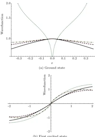
Figure 2 compares the numerically exact solu-tions of the un-normalized wave-funcsolu-tions. Here, the ground and rst excited states are shown versus the solution obtained by our proposed bases (Eq. (14)), improved WKB bases (Eq. (15)), and simple WKB basis cos(R0xk(t)dt). The superior accuracy of the solution by Eq. (14), close to the expansion point, is clearly visible in this plot. The improved WKB bases are highly erroneous for bounded modes as can be seen here, while simple WKB solutions are still less accurate than our proposed basis functions (Eq. (14)).
4. Conclusions
In summary, we presented a new pair of bases for solving the wave equation. Through several explicit examples, we have established the analytical power of the proposed basis functions and their advantage over WKB basis solutions. Our new basis functions are not divergent close to singularities at turning point and they maintain remarkable accuracy compared to the analytical solutions in the vicinity of expansion point. The basis functions also exactly satisfy the initial conditions.
Figure 2. Comparison of un-normalized ground state wave-functions for =1
2 within a subdomain of the range spanned by turning points [ ; +]: numerically exact (solid black); newly proposed basis functions (dashed); simple WKB (dot dashed); improved WKB (dotted). All solutions diverge at innity beyond the turning points, but the improved WKB bases diverge at the turning points.
References
1. Yariv, A., An Introduction to Theory and Applications of Quantum Mechanics, Dover (2013).
2. Khorasani, S. and Mehrany, K. \Dierential transfer matrix method for solution of one-dimensional linear non-homogeneous optical structures", J. Opt. Soc. Am. B, 20(1), pp. 91-96 (2003).
3. Mehrany, K. and Khorasani, S. \Analytical solution of non-homogeneous auisotropic wave equation based on dierential transfer matrices", J. Op. A: Pure Appl. Opt., 4(6), pp. 524-635 (2002).
4. Khorasani, S. and Adibi, A. \Analytical solution of linear ordinary dierential equations by dieren-tial transfer matrix method", Electron. J. Di. Eq., 2003(79), pp. 1-18 (2003).
5. Khorasani, S. \Dierential transfer matrix solution of generalized eigenvalue problems", Proc. Dynamic Systems & Appl., 6, pp. 213-222 (2012).
6. Wilcox, R.M. \Exponential operators and parameter dierentiation in quantum physics", J. Math. Phys., 8, pp. 962-982 (1967).
7. Khorasani, S. \Reply to comment on `analytical so-lution of nonhomogeneous anisotropic wave equation based on dierential transfer matrices'", J. Opt. A: Pure Appl. Opt., 5, pp. 434-435 (2003).
8. Khorasani, S. and Adibi, A. \New analytical approach for computation of band structure in one-dimensional periodic media", Opt. Comm., 216, pp. 439-451 (2003).
9. Zariean, N., Sarra, P., Mehrany, K. and Rashidian, B. \Dierential-transfer-matrix based on airy's functions in analysis of planar optical structures with arbitrary index proles", IEEE J. Quant. Electron., 44, pp. 324-330 (2008).
10. Khorasani, S. and Karimi, F. \Basis functions for solution of non-homogeneous wave equation", Proc. SPIE, 8619, 86192B (2013).
11. Schleich, W., Quantum Optics in Phase Space, Wiley-VCH, Berlin (2001).
12. Chui, S.T. and Lin, Z.F. \Long-wavelength behavior of two-dimensional photonic crystals", Phys. Rev. E, 78, 065601(R) (2008).
13. Khorasani, S., Applied Quantum Mechanics (in Per-sian), Delarang, Tehran (2010).
14. Sakurai, J.J., Modern Quantum Mechanics, Rev. Ed., Addison-Wesley (1993).
Biography
Sina Khorasani received the MSc and PhD degrees in Electrical Engineering from Sharif University of Technology, Tehran, in 1997 and 2001, respectively, where he is a Full Professor. He was with the School of Electrical and Computer Engineering at Georgia Institute of Technology as a Postdoctoral (2002-2004) and Research Fellow (2011-2012). He is now with Ecole Polytechnique Federale de Lausanne (2016-2017) as a Visiting Professor. His active research areas in-clude quantum optics and photonics, and quantum electronics. Dr. Khorasani is a Senior Member of IEEE.