Sharif University of Technology
Scientia IranicaTransactions A: Civil Engineering www.scientiairanica.com
Proposing a global sensitivity analysis method for
linear models in the presence of correlation between
input variables
Y. Daneshbod and M.J. Abedini
Department of Civil and Environmental Engineering, Shiraz University, Shiraz, Iran. Received 25 June 2012; received in revised form 21 June 2015; accepted 15 September 2015
KEYWORDS Sensitivity analysis; OAT;
Correlation; Local SA; Monte Carlo simulation.
Abstract. Sensitivity analysis is considered to be an important part of evaluating the performance of mathematical or numerical models. One-factor-at-a-time (OAT) and dierential methods are among the most popular Sensitivity Analysis (SA) schemes employed in the literature. Two major limitations of the above methods are lack of addressing the correlation between model factors and being a local method. Given these limitations, its extensive use among modelers raises concern over the credibility of the associated sensitivity analyses. This paper proposes proof for the ineciency of the aforementioned methods drawn from experimental designs, and provides a novel technique based on Principal Component Analysis (PCA) to address the issue of the correlation between input factors. In addition, proper guidelines are suggested to handle other conditions.
© 2016 Sharif University of Technology. All rights reserved.
1. Introduction
Sensitivity Analysis (SA) is the study of how the change in the output of a model can be attributed, qualitatively or quantitatively, to variation of dierent input variables, and of how the given model reacts upon the information passed into it. Based on this description, it is safe to conclude that SA is a necessary ingredient of model building in any setting, either diagnostic or prognostic, and in any discipline where models are called upon for design purposes [1]. Though this is a correct denition of SA, one may make false conclusion of thinking that SA is a tool specic for modelers. As a matter of fact, engineers as an end user of the developed models can benet from it as well. For example, consider an environmental engineer who intends to apply rainfall-runo model for a real-life problem. If this engineer knows which model input
*. Corresponding author.
E-mail address: [email protected] (M.J. Abedini)
parameter has more impact on model output results, a wise decision would be to spend much of the time and capital to dene carefully the most important parameters to predict the runo, precisely. Similar examples in engineering are easy to nd where SA could be helpful in decision-making.
There are a number of dierent methods of sen-sitivity analysis with each method having a unique exibility and functionality. As a result, dierent scientists have dierent ideas about categorizing SA methods. Frey and Patil [2] concentrate on methodol-ogy, classifying sensitivity analysis into mathematical, statistical, and graphic methods, while Ascough et al. [3] focus on capability, adopting the following classications; screening, local, and global SA methods. From a functional standpoint, sensitivity analysis can be divided into local and global SAs or, according to Morgan's denition, into deterministic and probabilis-tic [3,4].
Local SA concentrates on the local impact of the factors on the model. Local SA is usually carried
out by computing partial derivatives of the output function with respect to the input variables. The term `local' means that all derivatives are taken at a unique and well-dened point, known as `baseline value' or `nominal value', in the domain of the input factors. One can see local SA as a particular case of one-factor-at-a-time (OAT) method, whereby one factor is varied while all others are held constant at their respective nominal values. In contrast, the global sensitivity techniques examine the global response (averaged over the variation of all the parameters) of model output(s) by exploring a nite (or even an innite) region. Global sensitivity analyses are shown to be more eective when the predictor variable is inuenced by simultaneous changes in seemingly independent variables. This simultaneous variation would take into account the interaction among factors. Though global SA methods enjoy not having any of the local methods' limitations, they are much more complex and computationally expensive. The dierence between local and global SAs can be best examined in a simple nonlinear example. Let us examine the sensitivity of independent variables of X1and X2in a nonlinear function, Y = X12+X2. For
local SA, the sensitivity index of the two independent variables changes as the SA domain changes. The dependent variable is more sensitive to the variable X2 in the domain belonging to [0 - 1], while for all
other values, X1 is the dominant variable. In global
SA, regardless of domain, sensitivity index for X1 is
always greater.
In theory, local sensitivity analyses cannot be used to uncover the robustness of model based on inference unless the model is proven to be linear for the case of rst-order derivatives or, at least, additive for the case of higher and mixed-order derivatives. In other words, derivatives are informative at the nominal point where they are computed, but do not provide any additional information for the rest of the domain of input factors, except when some conditions, such as linearity or additivity, are provided in the mathematical model [5]. When the properties of the models are not known in advance, a global SA is recommended. This is why global SA methods are often called model-free by practitioners.
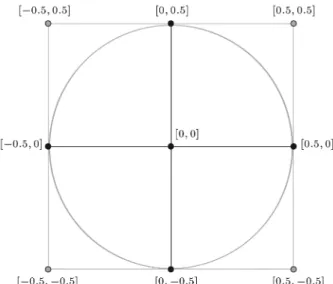
By reviewing recent literature associated with SA, it can be said that practitioners have acknowledged the importance of SA in approving or refuting a model-based analysis. Yet, regardless of its limitations, most of the sensitivity analyses were performed using an OAT approach [6]. Speaking of limitations, there are two concerns regarding OAT approach. First, OAT is non-explorative, which means as the number of the factors increases, the exploration feature decreases. As an example in Figure 1, it can be seen, clearly, that OAT explores only 5 points forming a cross, out of total 9 points [7]. By generalizing this example with a
Figure 1. The OAT method can only reach few points of the entire domain.
Figure 2. The curse of dimensionality; the volume ratio, ', of hyper-sphere to hypercube decreases quickly to zero as n number of dimensions increase.
geometrical explanation of the functional domain in n-dimensions, the n-cross will unavoidably be inscribed in a hyper-sphere. The problem is that this hyper-sphere represents a small percentage of the total functional domain dened by the hypercube. This is illustrated in Figure 1, where the explored cross is inscribed in the circle of center [0, 0] and radius of 0.5. In this 2-dimensional example, the ratio of the partially explored area to the total area is ' = 0:78. The exploratory domain quickly decreases as the number of dimensions increases (Figure 2). In 3 dimensions, it is ' = 0:52.
The general formula for the volume of the hyper-sphere of radius R in n dimensions is [8]:
Vn(R) =
n 2
(n 2 + 1)R
n or V
n(R) = CnRn; (1)
where is the gamma function. For even n, Cnreduces
to Cn =
n 2
(n
2)! and since
1 2
=p, for odd n, Cn = 2n+12 n 12
n!! , where n!! denotes double factorial.
ratio is ' = 0:000197. In the literature, this is known as curse of dimensionality or OAT paradox [5,9].
This limitation has been addressed by several practitioners; Saltelli [10] believes that \A good OAT would be one where after having moved one step in one direction, say along X1, one would directly take
another step along X2and so on, until all factors up to
Xk are moved of one step each during the rst stage."
This type of trajectory is known as `Elementary Eects' (EE) [10].
Another shortcoming related to OAT is that in the presence of correlation, OAT cannot detect interactions between factors, because this feature is based on the simultaneous movements of more than one factor. If factors move one at a time, the interactions are not triggered and, subsequently, not detected [5].
So, why modelers still prefer OAT? Arguments which might justify nominating OAT as a favorite candidate are:
(a) The SA is carried out in reference to baseline value, which is usually the most probable occurrence of the model in real world;
(b) This method requires much less computational ef-forts (i.e., CPU time) than any global SA method;
(c) Movement of one factor at a time means that whatever eect is observed on the output is due, exclusively, to that factor [5];
(d) It never assesses a non-important factor as impor-tant. This is also known as type I error [5];
(e) Since it deals with change of one parameter at a time, the chance of model failure decreases, as opposed to changing all factors. In case of model failure, the approach helps modeler to identify the factor responsible for model crash [5];
(f) The OAT approach is consistent with the mod-eler's way of changing one parameter at a time as he/she wants to verify, systematically, the eect of parameter variation.
To the best of the authors' knowledge, there is no deterministic SA method to address the interaction between factors in a comprehensive way (Morris's method is known to be global [1]). All of the SA methods, which produce reliable ranking in presence of correlation, are of probabilistic nature. These methods are not favored by end users due to their complexity and high computational cost. There is an ample need to have a simple method with no computational burden, yet powerful enough to address the correlation issue among the input variables involved. This study proposes a methodology based on standard OAT to extend its capability to address one of the limitations, which has long been subjected to extensive criticism.
Beyond the limitations of local SA methods, there are still situations where these methods fail to determine the correct order of importance among variables. Traditional modelers usually fail to notice them and perform perfunctory SA, clearly raising con-cerns regarding the developed models. This research also tends to address the common mistakes that may occur while performing OAT and dierential SA for linear models. Some guidelines will be suggested so that practitioners avoid these common pitfalls of the discussed SA methods.
2. Methodology
The most popular SA methods among scientists are dierential and OAT. Both are local SA methods, which explore sensitivity of the model around a narrow region of the feature space. First, methods are briey explained in the following sections. Later on, the pitfalls of the methods are revealed by performing a series of experiments. Suitable modications are introduced so that the practitioners avoid the common mistakes.
The benchmark for all of the experiments is Monte Carlo-based global SA, wherein 1000 samples are generated using random sampling. For examples, with correlated variables, the procedure proposed by Iman and Conover's method [11] is used to generate correlated samples. The SA index is Pearson product moment correlation coecient (PEAR), which is the usual linear correlation coecient computed among a pair of variables. For comparison purposes, the SA measures resulted from dierent techniques are normalized.
2.1. Standard OAT-SA
There are dierent avors of OAT according to Daniel [12], OAT methods can be classied into ve types:
(a) Strict OAT: This perturbs one factor from the condition of the last preceding model run;
(b) Paired OAT: This produces two observations and, therefore, one simple comparison at a time;
(c) Free OAT: In this type, each run can be performed under a new condition;
(d) Curved OAT: This produces a subset of results by perturbing only one easy-to-vary factor while others are held constant;
(e) Standard OAT: This perturbs one factor from a standard condition.
This research focuses on standard OAT, in which the standard condition is usually the average of input factors over their domain. This type of SA only addresses the sensitivity of model output relative to
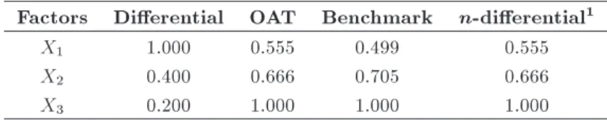
Table 1. Summary of sensitivity indexes.
Factors Dierential OAT Benchmark n-dierential1
X1 1.000 0.555 0.499 0.555
X2 0.400 0.666 0.705 0.666
X3 0.200 1.000 1.000 1.000
1Normalized dierential method.
a point where the parameters are held constant. The sensitivity measure is determined by calculating the ra-tio of model output while perturbing each parameter's value about the baseline value, in turn, to the nominal value of model output. The amount of parameter perturbation can either be a plus/minus percentage of their baseline value or one standard deviation of their distribution. The latter case has the advantage of taking into account the parameter's variability and the associated inuence on model output [13]. The main advantage of such methods is their low computational cost. Considering two values for each perturbed factor and an extra run for the nominal value of the model output, a model with K parameters requires 2K + 1 runs.
2.2. Dierential SA
Dierential analysis, also known as the direct method, is based on the behavior of the model while all param-eters are set to their mean value. It is based on partial dierentiation of the combined model. When a model is described by an explicit, closed algebraic equation, the sensitivity measure for a specic independent variable is estimated by partial derivative of the dependent variable with respect to the independent variable [13]. In the following subsections, a few case studies are introduced to highlight the pitfalls associated with traditional methods and, subsequently, a remedial measure is suggested for each approach.
2.3. Case 1: Where dierential SA fails A simple test model [1] shows that partial derivative of the output Y with respect to an input factor Xi at a
xed point fails to properly address the sensitivity of linear models. This study assumes that X1, X2, and X3
(the independent variables) are mutually independent and uniformly distributed in their respective range. The functional relationship between the dependent variable Y and the independent variables is:
Y =Xn
i=1
aiXi; (2)
where Xi U(xi i; xi+i), xi= 3i 1, and i= 0:5xi
are uniformly distributed in their range. Taking k = 3, the independent variables, constant coecients, and their computational domains are computed as follow:
X1 U(0:5; 1:5);
X2 U(1:5; 4:5);
X3 U(4:5; 13:5); (3)
Y = 5X1+ 2X2+ X3: (4)
Now, let us discuss the sensitivity of the dependent variable Y to each independent variable. According to the sensitivity analysis conducted based on the dier-ential method [14], all partial derivatives are constant as independent variables are mutually independent:
@Y @X1 = 5;
@Y @X2 = 2;
@Y
@X3 = 1: (5)
The sensitivities of the dependent variable to the inde-pendent variables are ranked as X1, X2, and X3, and
the value of each independent variable has no impact on the sensitivity coecient, i.e. ranking. Sensitivity analysis for the test case is carried out by two methods based on OAT and Monte Carlo sampling techniques. The results are summarized in Table 1.
As can be seen, the dierential method fails to rank the factors correctly. Even the simple OAT method is able to capture the ranks correctly. This is due to the fact that the dierential method does not consider the variation of input variables. An available practice to address these misleading results is to normalize the derivatives by standard deviations (reference). For a general linear model of Eq. (2), the sensitivity measure is:
S
Xi= Xi=Y
(@Y=@Xi) : (6)
Since for a linear modelPni=1 S Xi
2
= 1, S Xi
2 gives how much each individual factor contributes to the variance of the output of interest. This turns S
Xi to
be a hybrid local-global measure. After incorporating the suggested modication to the test case, the results improve as can be seen in Table 1. Though, quan-titatively, it is not in agreement with the benchmark values, it is now in a correct order.
2.4. Case 2: OAT and the range eect
Due to the local nature of OAT, the range and distri-bution of factors have no eect on the results obtained by the method. This will raise concerns when the dierences between ranges of factors are signicant or
Table 2. Summary of sensitivity measures. Factors S-OAT Benchmark OAT-SD1
X1 1 0.155 0.117
X2 0.8 1 1
1 OAT standard deviation perturbation.
the factors have dierent distributions. A test case has been set up to demonstrate this shortcoming.
Y = X1+ X2; (7)
X1 U(9; 11);
X2 U(1; 15): (8)
As it can be seen in Table 2, OAT method fails to rank the factors properly. This is because the sensitivity measure was determined by variation of input parame-ters with 20%. This methodology is unable to capture the eects of the computational domain and distribu-tion of factor. One way to overcome this limitadistribu-tion is to vary the input factors by one standard deviation of their input distribution rather than by 20%. The SA for Eq. (7) is repeated with the mentioned modication. Results have been improved. As can be seen, it is quite consistent with the benchmark ranking.
2.5. Case 3: The correlation eect (multi-collinearity)
When a question arises about which component of a linear model has more contribution to the model output, any SA method discussed earlier, depending on its conditions, is applicable. But when the linear independent assumptions are contravened, there will be doubt on the interpretability of regression coe-cients, which were decisive in earlier methods. Thus, performing SA on a linear model based on an ordinary least square will produce unlikely results.
A workaround to the stated problem is to sub-stitute least square with a reliable technique to build the desired linear model so that standardized regression coecients can be used for SA. The suggested tech-nique is based on component analysis, which converts a set of correlated variables into a set of linearly un-correlated variables by an orthogonal transformation. The method will be discussed in detail in the following section.
As the rst step, we state our linear model of Eq. (2) as a relationship of y to '.
y = 1'1+ 2'2+ 3'3+ ::: + k'k; (9)
in which 'k are a set of orthogonal variates (principal
components) from linear combination of xis, where k <
n; k is the number of principal components; y and xi
are standardized values of the original variables (Y; Xi)
with zero mean and unit variance:
'1= m11x1+ m21x2+ m31x3+ ::: + mn1xn;
'2= m12x1+ m22x2+ m32x3+ ::: + mn2xn;
'3= m13x1+ m23x2+ m33x3+ ::: + mn3xn;
...
'k= m1kx1+ m2kx2+ m3kx3+ ::: + mnkxn; (10)
where mij is a typical i component of j eigenvector
corresponding to the predictor variates correlation matrix.
Substituting Eq. (10) into Eq. (9) results in: y = (1m11+ 2m12+ 3m13+ ::: + km1k) x1
+ (1m21+ 2m22+ 3m23+ ::: + km2k) x2
+ (1m31+2m32+3m33+:::+km3k) x3+:::
+ (1mn1+ 2mn2+ 3mn3+ ::: + kmnk) xn:
(11) If the numerical values of the parameter in the paren-thesis could be calculated, Eq. (11) expresses a linear relation between y and xi. We have already discussed
how to compute mij. As for i, Eq. (9) is a regression
equation with independent variables, k could be
com-puted by ordinary least square. Simultaneous normal equations resulted from OLS are given by:
1
X '2
1+ 2
X
'1'2+ 3
X '1'3
+ ::: + k
X
'1'k =
X '1y;
1
X
'1'2+ 2
X '2
2+ 3
X '2'3
+ ::: + k
X
'2'k =
X '2y;
1
X
'1'3+ 2
X
'3'2+ 3
X '2
3
+ ::: + k
X
'2'k =
X '3y;
... 1
X
'1'k+ 2
X
'k'2+ 3
X 'k'3
+ ::: + k
X '2
k =
X
'3y: (12)
Since 'i are orthogonal, all theP'i'k terms with i 6=
respective variances are equal to eigenvalue i, which in
turn is equivalent to P'2
i. After some manipulation,
k are:
1=
P '1y
P '2
1 =
P '1y
1 ;
2=
P '2y
P '2
2 =
P '2y
2 ;
3=
P '3y
P '2
3 =
P '3y
3 ;
... k =
P 'ky
P '2
k =
P 'ky
k : (13)
Multiplying both sides of Eqs. (11) by y and adding them up results in:
X
'iy =m1k
X
x1y + m2k
X
x2y + m3k
X x3y
+ ::: + mnk
X
xny: (14)
Making use of Eqs. (14) and (15), and noting that for standardized variate,Pxiy equals their correlation
coecient rxiy, s can be simply computed from the
following equations:
1=(1=1) m11rx1y+ m21rx2y+ m31rx3y
+ ::: + mn1rxny
;
2=(1=2) m12rx1y+ m22rx2y+ m32rx3y
+ ::: + mn2rxny
;
3=(1=3) m13rx1y+ m23rx2y+ m33rx3y
+ ::: + mn3rxny
; ...
k =(1=k) m1krx1y+ m2krx2y+ m3krx3y
+ ::: + mnkrxny
: (15)
Now that the coecients of the linear model in Eq. (11) can be calculated, these coecients can be attributed to their sensitivity ranking.
It is worth mentioning that selecting the right number of principal components in Eq. (10), i.e. k, is an important step in this method. Small eigenvalues corresponding to the last few principal components
cause high variance in regression coecient, which, in turn, results in unstable coecients [15]. Repeating the calculation similar to Eq. (11) by using all of the is is
equivalent to performing OLS (ordinary least square), for which its consequences were mentioned and assessed earlier. There are dierent criteria to choose with regard to which and how many principal components should be retained. We chose a criterion whereby the set of largest k contributors were selected to achieve and meet the following inequality:
1:0 > Pk
i=1i
n 0:85: (16)
Note that i is the eigenvalues and n is total number
of eigenvalues.
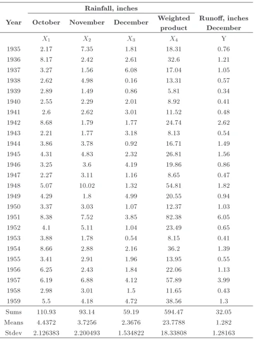
To justify the robustness of the proposed method, a linear model is t on rainfall-runo data for the White Hollow watershed from years 1935 to 1959 presented in Table 3 [16]. The rainfall data from three consecutive months October, November, and December of each year and the associated December runo are considered. Furthermore, an assumptive weighted cross product of rainfall for the given months is introduced into the model as a strong correlated predictive variable.
The correlation matrix for the predictive variables is as follows:
2 6 6 4
1 0:14 0:17 0:70 0:14 1 0:06 0:69 0:17 0:06 1 0:34 0:70 0:69 0:34 1
3 7 7 5
As can be seen, there is a strong positive correlation between variable 4 and others.
Three SA methods are preformed: dierential analysis on OLS, the proposed method, and the bench-mark. The results are summarized in Table 4.
As can be seen in Table 4, dierential analysis fails to capture the interaction between the factors when the model is based on OLS. As a result, sensitivity measure is not consistent with the benchmark ranking. On the other hand, the proposed method demonstrates promising results, which are in good agreement with benchmark results. The main feature of this method that may have a great appeal for practitioners is that it can be performed systematically with much low computational burden compared to Monte Calro-based simulation methods.
3. Conclusion
Complex SA methods probably redound to more accu-rate conclusions, but their complexity discourages the modelers from implementing them; so, they are lured to use less credible methods such as OAT and dierential
Table 3. Monthly rainfall-runo, white hollow watershed. Rainfall, inches
Year October November December Weighted product
Runo, inches December
X1 X2 X3 X4 Y
1935 2.17 7.35 1.81 18.31 0.76
1936 8.17 2.42 2.61 32.6 1.21
1937 3.27 1.56 6.08 17.04 1.05
1938 2.62 4.98 0.16 13.31 0.57
1939 2.89 1.49 0.86 5.81 0.34
1940 2.55 2.29 2.01 8.92 0.41
1941 2.6 2.62 3.01 11.52 0.48
1942 8.68 1.79 1.77 24.74 2.62
1943 2.21 1.77 3.18 8.13 0.54
1944 3.86 3.78 0.92 16.71 1.49
1945 4.31 4.83 2.32 26.81 1.56
1946 3.25 3.6 4.19 19.86 0.86
1947 2.27 3.11 1.16 8.65 0.47
1948 5.07 10.02 1.32 54.81 1.82
1949 4.29 1.8 4.99 20.55 0.94
1950 3.37 3.03 1.07 12.37 1.03
1951 8.38 7.52 3.85 82.38 6.05
1952 4.1 5.11 1.04 23.49 0.65
1953 3.88 1.78 0.54 8.15 0.41
1954 8.66 2.88 2.16 36.2 1.39
1955 3.41 2.91 1.96 13.95 0.55
1956 6.25 2.43 1.84 22.06 1.13
1957 6.19 6.88 4.12 57.89 3.99
1958 2.98 3.01 1.5 11.65 0.43
1959 5.5 4.18 4.72 38.56 1.3
Sums 110.93 93.14 59.19 594.47 32.05
Means 4.4372 3.7256 2.3676 23.7788 1.282
Stdev 2.126383 2.200493 1.534822 18.33808 1.28163 Table 4. Summary of sensitivity measures.
Factors OLS based
model Benchmark
Proposed method
X1 0.58 0.84 0.90
X2 1 0.62 0.57
X3 0.52 0.38 0.36
X4 0.37 1 1
analysis. The limitations of these methods have been clearly pointed out in the literature. First, being a local method, meaning that the sensitivity of the model output is analyzed only at a single point and second, lack of ability to address the interaction among input factors.
A novel global SA method has been presented in
this paper to deal with the interaction limitation. The interaction among the correlated data is captured in a linear model by taking advantage of principal compo-nents. The method can be implemented systematically with low computational cost. An example shows that the proposed method succeeds where common methods fail to justify the proper ranking.
Besides these limitations, there are few other situations, where if not paid enough attention, common SA methods result in false analysis. This paper designed a number of experiments to demonstrate the ineciency of these methods.
In Case 1, when distribution of predictor variables is not taken into account, dierential SA method fails to rank the factors correctly. The proper adjustment has been advised to overcome this concern.
Case 2 was designed to demonstrate the ine-ciency of OAT method in common practice, especially when the predictor variables have high proportions of variance.
Case 3 was designed to demonstrate the ability of the proposed method to handle the correlation between predictor variables in a linear model, where the reviewed methods failed to capture. Although it is proposed for linear models, its implementation for nonlinear cases should not be ruled out. Research is underway to address this issue in subsequent publica-tions.
References
1. Saltelli, A., Chan, K. and Scott, E.M., Sensitivity Analysis, In Wiley Series in Probability and Statistics, John Wiley and Sons, New York (2008).
2. Frey, C.H. and Patil, S.R. \Identication and review of sensitivity analysis methods", Risk Analysis, 22(3), pp. 553-578 (2002).
3. Ascough II, J.C., Green, T.R., Ma, L. and Ahjua, L.R. \Key criteria and selection of sensitivity analysis methods applied to natural resource models", Modism International Congress on Modeling and Simulation, Modeling and Simulation Society of Australia and New Zealand, Melbourne, pp. 2463-2469 (2005).
4. Morgan, M.G., Henrion, M. and Small, M., Un-certainty: A Guide to Dealing With Uncertainty in Quantitative Risk and Policy Analysis, Cambridge University Press (1992).
5. Saltelli, A. and Annoni, P. \How to avoid a perfunctory sensitivity analysis", Environ. Model. Softw., 25(12), pp. 1508-1517 (2010).
6. Saltelli, A., Ratto, M., Tarantola, S. and Campolongo, F. \Sensitivity analysis practices: Strategies for model-based inference", Reliability Engineering & System Safety, 91(10-11), pp. 1109-1125 (2006).
7. Vidal, C., Articial Cosmogenesis: A New Kind of Cosmology, in Irreducibility and Computational Equiv-alence: Wolfram Science 10 Years After the Publi-cation of A New Kind of Science, Zenil, H. (Ed.), arXiv:1205.1407v1 (2012).
8. Huber, G., Gamma Function Derivation of n-Sphere Volumes, The American Mathematical Monthly, 89(5), pp. 301-302 (1982).
9. Asserina, O., Loredob, A., Petelet, M. and Iooss, B. \Global sensitivity analysis in welding simulations-What are the material data you really need?", Finite Elements in Analysis and Design, 47(9), pp. 1004-1016 (2011).
10. Saltelli, A., Ratto, M., Andres, T., Campolongo, F., Cariboni, J., Gatelli, D., Saisana, M. and Tarantola, S.,
Global Sensitivity Analysis: The Primer, John Wiley and Sons, New York (2008).
11. Iman, R.L. and Conover, W.J. \A distribution-free approach to inducing rank correlation among input variables", Communications in Statistics, Simulation and Computation, 11(3), pp. 311-334 (1982).
12. Daniel, C. \One-at-a-time plans", Journal of the American Statistical Association, 68(342), pp. 353-360 (1973).
13. Hamby, D.M. \A comparison of sensitivity analysis techniques", Health Phys., 68(2), pp. 195-204 (1995).
14. Turanyi, T. and Rabitz, H. \Local methods and their applications", in Sensitivity Analysis, Saltelli, A., Chan, K. and Scott, E.M., Editors, John Wiley and Sons, New York (2008).
15. Rencher, A.C., Multivariate Statistical Inference and Applications, In Wiley Series in Probability and Statis-tics, John Wiley and Sons, New York (1998).
16. Snyder, W.M. \Some possibilities for multivariate analysis in hydrologic studies", J. Geophys. Res., 67(2), pp. 721-72 (1962).
Biographies
Younes Daneshbod was born in Shiraz, Iran, in 1974. He received a BS degree (1996) in Civil Engineering and an MS degree (2000) in Hydraulic Structures both from Shiraz University, Iran. He is currently a PhD candidate in the department of Civil and Environmental Engineering at Shiraz University. In 2004, he joined the Department of Civil Engineer-ing at the Islamic Azad University, Arsanjan branch (IAUA), as a Lecturer and, subsequently, served as the head of the Department of Civil Engineering for two consecutive terms. His research interests include sensitivity analysis, uncertainty analysis, and articial intelligence applied to civil engineering problems. He is the Life Member of the Iran Construction Engineering Organization (IRCEO) and a recipient of the IAUA Distinguished Researcher Award (2008).
Mohammad Javad Abedini was born in 1958, in Shiraz, Iran. He obtained his BS and MS degrees in Civil Engineering and Hydraulic Structures from Shiraz University, Iran, in 1985 and 1991, respectively, and his PhD degree in Water Resources Engineering from the University of Guelph, Canada, in 1998. He is currently Professor in the Department of Civil and Environmental Engineering at Shiraz University, Iran. His research interests include computational hydrology and hydraulics, analysis of temporal and spatial series, and data assimilation.