Constructive reverse investigations into differential equations
HANNESDIENER IRISLOEB
Abstract: We study Picard’s Theorem and Peano’s Theorem from a constructive reverse perspective. This means that we have to change our focus from global properties to local properties. We also extend the theory ofpointwisecontinuously differentiable functions to include Rolle’s Theorem, the Mean Value Theorem, and the full Fundamental Theorem of Calculus.
2000 Mathematics Subject Classification03F60, 26E40 (primary); 03F55 (sec-ondary)
Keywords: constructive mathematics, reverse mathematics, differentiation, differ-ential equations, pointwise analysis
1
Introduction
Under the program of constructive reverse mathematics, many theorems have been proven equivalent over Bishop’s constructive mathematics (BISH) to the Uniform Continuity Theorem [12,14]:
UCT Every pointwise continuous mapping of a compact1metric space into a metric space is uniformly continuous.
By buildingUCTinto his definition of continuity, Bishop elegantly circumvented the decision of whether to accept it as a principle or not. In his own words he deemed “the concept of a [pointwise] continuous function [. . .] not relevant” [9, p. 3]. In the same fashion, Bishop focused on functions that are differentiable in a uniform way, and was not interested in pointwise differentiability. We believe that the contrast of pointwise versus uniform properties for continuity and differentiability is interesting.
In the tradition of Bishop we make free use of the axiom of countable and dependent choice. We will, however, explicitly mention this in these occasions
1Following common practice in constructive mathematics, we take totally boundedness
This paper has three goals. The first being to contribute to the program of constructive reverse mathematics. The second, related goal, is to highlight and understand the difference between local and uniform definitions of continuity and differentiability. The third goal is to, within BISH, prove theorems using pointwise definitions of differentiability; thus continuing work begun in [18]. Although we are thus working in Bishop-style informal mathematics, we believe that this research could be carried out in a suitable formal framework like IZF [15,4], CZF [3], or HAω [25,26].
Section2studies two varieties ofUCT. They both turn out to be equivalent and will play a role in the rest of the paper. In Section3we investigate pointwise differentiability. A constructive proof of Rolle’s Theorem without additional assumptions, commonly made in the constructive literature, is presented.
In Section4and5we prove that versions of Picard’s Theorem and Peano’s Theorem are equivalent toUCT. As far as we know, these are the first results on differential equations in constructive reverse mathematics. For some other results on constructive existence of solutions of differential equations see e.g. [16], which deals amongst other things with Euler’s method.
Being equivalent toUCT, there is no hope to prove these theorems in the framework of Russian Recursive Mathematics. In the last section we will strengthen this result and produce strong counterexamples. That means we will actually give an example of a recursive function for which these theorems fail to hold.
2
Uniform Continuity Theorems
Since there are many different notions of continuity commonly in use, we will specify the definitions we have in mind when talking about continuity throughout this paper.
Definition 1 Consider two metric spaces (X,dX) and(Y,dY). A function f :X→Y
is called continuous, if for all x∈X and for allε >0there existsδ >0 such that for allx0∈X
dX x0,x
< δ =⇒ dY f(x),f(x0)
< ε.
Furthermore, it is called uniformly continuous, ifδ does not depend onx.
First, we prove an extension result for pointwise continuous functions that is needed later, but is also of interest by itself.
Lemma 2 Consider an arbitrary metric space(X,dX) and a complete metric space
(Y,dy). Furthermore assume thatD⊂X is a dense subset and f :D→Y a function
such that for everyx∈X andε >0 there existsδ >0with
(1) ∀y,z∈D((dX(x,y)< δ∧dX(x,z)< δ) =⇒ dY(f(y),f(z))< ε).
Then there exists a unique continuous function˜f :X →Y such that f˜(x)=f(x) for all
x∈D.
Proof Since Dis dense, for every x ∈X we can find a sequence (xn)n>1 inD that
converges tox. Property (1) now ensures that (f(xn))n>1is Cauchy and hence converges.
Furthermore, the limit is not dependent on the choice of the sequence (xn)n>1, and thus
it makes sense to denote this limit by ˜f(x).2 Using unique choice we get a function ˜f, which is continuous: for letx∈X andε >0 be arbitrary. Chooseδ >0 such that (1) is satisfied. Now considery∈X such thatdX(x,y)< δ. By the construction of ˜f we
can findx0 ∈D and y0 ∈D withd(x0,x)< δ and d(y0,y)< δ. By (1) we therefore havedY(˜f(x),f(x0))< ε,dY(˜f(y),f(y0))< εandd(f(x0),f(y0))< ε. It follows that
dY(˜f(x),˜f(y))6dY(˜f(x),f(x0))+dY(f(x0),f(y0))+dY(f(y0),f˜(y))63ε,
whence ˜f is continuous. Since for anyx∈Dthe constant sequence (x)n>1 converges
tox, also ˜f(x)=f(x). To see that ˜f is unique, consider another continuous function g:X →Y such thatf(x)=g(x) for all x∈D. Now assume that d(˜f(x0),g(x0))>0 for somex0∈X. Then, because we are dealing with continuous functions, there exists
a neighbourhoodU ofx0 such thatd(˜f(x),g(x))>0 for allx∈U. SinceD is dense,
the intersectionD∩U is inhabited and we get a contradiction; so ˜f =g.
Working within BISH, we are interested in the following three principles, wherea,b are real numbers witha<b:
UCT[a,b] Every continuous function f : [a,b] → R is uniformly
continuous.
2Here countable choice is used in choosing a sequence (x
n)n>1. This is, however, for
convenience only. Countable choice is avoidable here, if one used Dedekind reals (more details can be found in [17]). One could then define
˜
f(x)=\
n∈N
y∈Y| ∃z∈X
|x−z|<1
n ∧y<f(z)
.
Property (1) ensures that this set is order located, which is an additional requirement on a Dedekind real in the constructive treatment.
BUCT[a,b] Every bounded, continuous function f : [a,b] → R is
uniformly continuous.
LUCT[a,b] Every continuous functionf : [a,b]→Ris locally uniformly
continuous.
Wherelocally uniformly continuousis defined as follows:
Definition 3 A continuous function f : [a,b]→Rislocally uniformly continuous, if for every x ∈ [a,b] there exists h > 0 such that f is uniformly continuous on
[x−h,x+h]∩[a,b].
From [12] we know that UCT[0,1] is equivalent to UCT. Since every continuous
function is locally bounded, the following implications hold
UCT =⇒ BUCT[a,b] =⇒ LUCT[a,b].
We prove the reverse implications for functions defined on the unit interval. The general cases easily follow by scaling. In order to prove the next implication we first introduce the following principle:
AS[0,1] If (xn)n>1 is a sequence of real numbers that is bounded away
from every point in [0,1] then (xn)n>1 is eventually bounded away from
the entire interval.
In [6], this principle has been shown to be equivalent to a version of Brouwer’s Fan theorem, which itself is weaker thanUCT[5], but stronger than the Fan theorem for decidable bars.3 This means, in particular, that together with Corollary 3.4 in [13, Chapter 2]AS[0,1] implies:
POS Every positively valued, uniformly continuous functionf : [0,1]→
Rhas a positive infimum.
We will show thatBUCT[0,1] is enough to show thatAS[0,1] holds.
Lemma 4 If (xn)n>1 is a sequence in R that is bounded away from every point in
[0,1], then there exists a subsequence(xkn)n>1 such that for alln∈None can decide
whether
xkn ∈[0,1]∨xkn ∈/ [0,1],
3It is an open question in constructive reverse mathematics, whether any of these implications
and there exist positive numbers(εn)n>1 such that for all n,m∈Nwith m>n
(2) xkn ∈[0,1]∧xkm ∈[0,1]
=⇒ |xkn −xkm|> εn.
Furthermore(xkn)n>1 is bounded away from[0,1]if and only if(xn)n>1 is.
Proof Let (xn)n>1 be a sequence inRthat is bounded away from every point in [0,1].
Since (xn)n>1 is bounded away from 0 and 1, there exists N such that for alli>N we
can decide
xi∈[0,1]∨xi∈/ [0,1].
Now, with the help of dependent choice, define a subsequence the following way: start by setting k1 =N. Assume we have constructed kn for somen. If xkn ∈/ [0,1] let
kn+1=kn+1. If xkn ∈[0,1] there existsεn>0 andkn+1 such that for all i>kn+1
|xkn−xi|> εn.
Clearly, the so defined subsequence satisfies (2). Now assume that there existsM such that
(3) xki ∈/ [0,1] for alli>M.
Then there cannot be a j>kM withxj ∈[0,1]: for assume such a jexists. Then find
j0 =min{i:kM <i6j∧xi ∈[0,1]}.
The construction therefore ensures that xkM+(j0−
kM) =xj0 ∈[0,1];
a contradiction to (3), and thusxj∈/ [0,1] for allj>kM. Since (xn)n>1 is also bounded
away from 0 and 1, the sequence is bounded away from the entire interval.
Lemma 5 BUCT[0,1] impliesAS[0,1] (and therefore POS).
Proof Given a sequence (xn)n>1 that is bounded away from every point in [0,1],
construct a subsequence and (εn)n>1 as in Lemma4. Furthermore, we may, perforce,
assume thatεn is decreasing. Since (xn)n>1 is bounded away from every point in [0,1]
we may also assume that ifxkn ∈[0,1] then 0<xkn−εn <xkn+εn <1. This ensures
that for any givenx∈[0,1] at most one term of the sum X
n:xkn∈[0,1]
max
0,
1−2(xkn −x) εn
is nonzero. The so defined functionf : [0,1]→Ris easily seen to be well-defined and continuous, and, furthermore, satisfies 06f 61. We can therefore applyBUCT[0,1]to
ensure thatf is uniformly continuous. So there exists N∈Nsuch that forx,y∈[0,1]
(4) |x−y|<2−N =⇒ |f(x)−f(y)|< 1 2.
Now assume that there exists n > N such that xn ∈ [0,1]. Then f(xn) = 1 and
f(xn+εn/2)=0 a contradiction to (4). Hencexn ∈/ [0,1] for all n>N, and since
(xn)n>1 is also eventually bounded away from 0 and 1, it is eventually bounded away
from the entire interval [0,1].
Proposition 6 BUCT[0,1] =⇒ UCT[a,b]
Proof Consider a continuous functionf : [a,b]→R. With the work in [12], it suffices
to show that f is bounded. Since f is continuous, so is the functiong : [a,b]→R defined by
g(x)= 1
max{1,|f(x)|}.
By virtue of the construction ofg, the following inequalities hold: ∀x∈[a,b](0<g(x)61).
As we assumeBUCT[0,1], gis uniformly continuous. Also, using Lemma5, we can
find anε >0 such that
∀x∈[0,1](ε <g(x)61). So|f|is bounded by max{ε−1,1}.
The more interesting implication is
Proposition 7 LUCT[0,1] =⇒ BUCT[0,1]
Proof Let f : [0,1] → R bounded and continuous. Furthermore, without loss of generality, we assume thatf(0)=f(1)=0 and that 06f 61. LetIn denote the open
interval (1−21n,1−2n1+1). For anyx∈In, we defineg(x) to be
1 2n+1f(2
n+1x−2(2n−
1)).
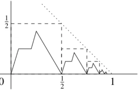
Lemma2yields the existence of a continuous map ˜g: [0,1]→R, such that ˜g(x)=g(x) for allx∈In and, furthermore, ˜g61−x. Figure1is an illustration of the idea behind
the construction of the function ˜g. Now because we assumeLUCT[0,1], there exists
N such that ˜g is uniformly continuous on [1−2N−1,1]. Since f = h◦g˜ ◦h0 for some linear, and therefore uniformly continuous, functionsh,h0, we conclude thatf is uniformly continuous.
0 1 2
1 1
2
Figure 1: Construction of the function ˜g.
We have now proved thatLUCT[a,b] is equivalent toUCT. We can easily generalise
this result to arbitrary (compact) metric spaces andLUCTas follows. Let (X, ρ) be a compact metric space andY be a metric space.
Definition 8 A continuous function f : X → Y is locally uniformly continuous, if for every x ∈ X there exists h > 0 such that f is uniformly continuous on
{y∈X|ρ(x,y)6h} ∩X.
LUCTis the following principle:
LUCT Every continuous function of a compact metric space into a metric space is locally uniformly continuous.
The following implications can now be seen to hold:
UCT =⇒ LUCT =⇒ LUCT[0,1] =⇒ UCT.
SoUCTandLUCTare equivalent. We will use this in the Sections4and5.
3
Differentiation
Just like we do not restrict our view to functions that are uniformly continuous (on compacts), we will not presuppose that every differentiable function on a compact interval is uniformly differentiable either.
Definition 9 Let f be a continuous function on[0,1]. We say that f isdifferentiable
if there exists a continuous functiongon[0,1]such that for eachx in[0,1]andε >0, there existsδ >0such that ify in[0,1]and|x−y|< δ, then
|f(y)−f(x)−g(x)(y−x)|6ε|y−x|.
Iff is a differentiable function, we will often write its derivative asf0. Note that every function has at most one derivative.
To contrast this version of differentiability with the two uniform ones that we will see later, we will also call itcontinuous differentiabilityto emphasise that the derivative is (pointwise) continuous, or pointwise differentiability, to stress thatδ depends on x. Rolle’s theorem is vital for the development of Analysis. The classical version states that iff : [a,b]→ Ris continuously differentiable and f(a)= f(b)=0, then there exists a pointξ∈[a,b] such that f0(ξ)=0. It is not surprising that one cannot hope to find a constructive proof of this theorem. In fact, a Brouwerian counterexample can be found in [24]. Nevertheless, there is hope to prove the following approximate version.
Theorem 10 If f : [a,b]→ R is continuously differentiable and f(a)= f(b)=0,
then for everyε >0there existsx∈[a,b]with |f0(x)|< ε.
Unfortunately the proof in [9] assumes that the function is differentiable in a uniform way. Recursive proofs, such as the one found in [2], make use of an unbounded search to find a point that satisfies the conclusion. Using dependent choice we can give a proof without any of these additional assumptions. To our knowledge this is the first such proof. First, though, we need to establish some lemmas.
Lemma 11 Iff : [a,b]→Ris continuously differentiable such thatf0(x)> εfor all
x∈[a,b] then it is impossible thatf(a)>0andf(b)<0.
Proof Aberth’s proof applies [2, Theorem 8.1].
Lemma 12 If f : [a,b]→ Ris continuously differentiable and x∈[a,b]such that
|f0(x)| > 0, then for each δ > 0 there exists y ∈ [a,b] such that |x−y| < δ and
|f(x)−f(y)|>0.
Proof We first look at the case thatf0(x)>0. Letδ >0. By the continuity off0, we can findδ0 >0 such that if |z−x|6δ0, then f0(z)>0. Take
y:=x+min{δ, δ0}.
We now apply Corollary 3 of [18] on the interval [x,y]. This gives us thatf(y)>f(x). The proof of the case thatf0(x)<0 is analogous and thus omitted.
Corollary 13 If f : [a,b]→ R is continuously differentiable and x ∈ [a,b] such thatf0(x)>0, then for eachδ >0 there existsy ∈[a,b]such that |x−y|< δ and
Proof Follows from Lemmas11and12.
We now are in a position to prove Theorem10.
Proof Let ε > 0. We may assume that |f0(a)| > ε/2 and |f0(b)| > ε/2, since otherwise we are done. In the cases thatf0(a)> ε/2 andf0(b)< ε/2 orf0(a)< ε/2 andf0(b)> ε/2 we can apply an approximate version of the intermediate value theorem [13] to the continuous functionf0 to find anx∈[a,b] such that|f0(x)|< ε. So let us, without loosing generality, assume that bothf0(a)> ε/2 and f0(b)> ε/2.
The idea of the rest of the proof is to use a suitably modified interval halving procedure to obtain two sequences (an)n>1 and (bn)n>1 and at the same time a binary sequence
(λn)n>1, which keeps track whether a point with the desired property is found. If this
happens the sequence (λn)n>1 becomes 1 from then on and the sequences (an)n>1 and
(bn)n>1 stabilise on this point. Of course we know that it is impossible that this never
happens. Working without the assumption of Markov’s principle though we have to, at least implicitly, produce a bound for this event. This is achieved, by choosing (an)n>1
and (bn)n>1 to converge to a pointy, which either has the desired property anyway or
for whichf0(y) and continuity around this point contains enough information to find this bound.
Using dependent choice, we define a binary sequence (λn)n>1 and two sequences of
real numbers (an)n>1 and (bn)n>1 such that for everyn∈N
(1) an6an+1 6bn+16bn;
(2) |bn−an|6 23
n
|b−a|;
(3) λn=0 implies thatf(an)>0>f(bn),f0(an)> ε/2 ,f0(bn)> ε/2 andan<bn;
(4) λn=1 implies that there existsx∈[a,b] such that|f0(x)|< ε.
Notice that, sincef0(a)>0, it follows from Corollary13that there existsa0∈[a,b] such thatf(a0)>0. Similarly there existsb0∈[a,b] with f(b0)<0. Again we might
assume that f0(a0)> ε/2 and f0(b0)> ε/2, since otherwise we are done. Also set
λ0 =0.
Now assume we have constructedλn,an and bn for some n>0. If λn =1 simply set
λn+1=1, an+1=bn+1=an. Ifλn=0 considerξ=(an+bn)/2. Either |f0(ξ)|< ε,
f0(ξ)< ε/2 orf0(ξ)> ε/2. In the second case we can use an approximate version of the intermediate value theorem to findx∈[a,b] with |f0(x)|< ε. So in the first two cases setλn=1,an+1=bn+1=an. In the third case we can use Lemma12to find a pointξ0
such that|ξ−ξ0|< 16|bn−an|and f(ξ)6=f(ξ0). Now either|f(ξ)|>0 or|f(ξ0)|>0.
We will only deal with the first possibility, since the second possibility can be dealt with in an almost identical fashion. Once more we may assume thatf0(ξ)> ε/2, because the other possibilities are obvious. Iff(ξ)>0 set λn+1=0, an+1=ξ and bn+1=bn.
Iff(ξ)<0 setλn+1=0, an+1=an andbn+1 =ξ. Properties (1) and (2) ensure that
the so defined sequences (an)n>1 and (bn)n>1 are Cauchy, and converge to the same
limity∈[a,b]. For the final time, we may assume thatf0(y)> ε/2, since we are done in the other cases. Sincef0 is continuous we can findδ >0 such thatf0(z)> ε/3 for allz∈[a,b] with|z−y|< δ. ChooseN such that [aN,bN]⊂By(δ). NowλN =0
leads to a contradiction to Lemma11and hence λN =1 and we are done.
Corollary 14 (Mean Value Theorem) If f : [a,b]→Ris continuously differentiable
anda<b, then for every ε >0there exists x∈[a,b] with
f0(x)−f(b)−f(a) b−a
< ε.
Proof Apply Rolle’s theorem10to
g(x)=f(x)−f(a)−f(b)−f(a)
b−a (x−a).
The next notion that we introduce,uniform differentiability, coincides with Bishop’s notion of differentiability in [9], if we would suppose that the functions involved are uniformly continuous.
Definition 15 Letf be a continuous function on[0,1]. We say that f isuniformly differentiableif there exists a continuous functiongon[0,1]such that for each ε >0
there existsδ >0such that ifx,yin[0,1]and|x−y|< δ, then
|f(y)−f(x)−g(x)(y−x)|6ε|y−x|.
However, a definition in the spirit of Bishop is not the only thinkable restriction of Definition9to some kind of uniformity.
Definition 16 Letf be a continuous function on[0,1]. We say that f isuniformly continuously differentiable if the function f is differentiable and its derivative is uniformly continuous.
It is not difficult to see that uniformly continuous differentiability follows from uniform differentiability. See also Proposition 2.2 in Chapter 6 of [25]. In fact both notions are equivalent.
Theorem 17 Every real-valued function on[0,1] is uniformly differentiable if and only if it is uniformly continuously differentiable.
Proof Letf : [0,1]→Rbe a uniformly differentiable function. Letε >0. Determine δ >0 such that for allx,y∈[0,1], if|x−y|< δ, then
|f(y)−f(x)−f0(x)(y−x)|< 1
2ε|y−x|.
Letx,y∈[0,1] such that|x−y|< δ. Suppose now that|x−y|>0; we see that: (f0(x)−f0(y))(x−y)=−f0(x)(y−x)−f0(y)(x−y)
=(f(y)−f(x)−f0(x)(y−x))+
(f(x)−f(y)−f0(y)(x−y)) 6|f(y)−f(x)−f0(x)(y−x)|+
|f(x)−f(y)−f0(y)(x−y)| 62·1
2 ·ε|y−x|=ε|y−x|. Similarly
(f0(x)−f0(y))(y−x)6ε|y−x|.
Hence|f0(x)−f0(y)||y−x|6ε|y−x|. So for all n∈N+ we have:
|f0(x)−f0(y)||y−x| |y−x|+n−1 6
ε|y−x| |y−x|+n−1.
By taking the limit (n→ ∞) we conclude that|f0(x)−f0(y)|< ε. This shows that a uniformly differentiable function is uniformly continuously differentiable.
Conversely assume thatf : [0,1]→Ris uniformly continuously differentiable, and let ε >0 be arbitrary. Since f0 is uniformly continuous there existsδ >0 such that for all x, ξ ∈[0,1]
|x−ξ|< δ =⇒
f0(x)−f0(ξ)< ε 2.
Now assume thatx,y∈[0,1] are such that|y−x|< δ. Assume that|x−y|>0. Then by Corollary14, there exists ξ such that|x−ξ|<|x−y|< δ and
f0(ξ)−f(y)−f(x) y−x
< ε 2.
Thus
f0(x)−f(y)−f(x) y−x
< ε. Multiplying the last equation with|y−x|gives
(5) f(y)−f(x)−f0(x)(y−x)6ε|y−x|. Notice that the function
g(x,y) :=f (y)−f(x)−f0(x)(y−x)−ε|y−x| is continuous and thatg(x,y)60 on a dense subset of
{(x,y)∈[0,1]2:|x−y|6δ}.
We can therefore conclude thatg(x,y)60 for all x,y with|x−y|6δ. Thus Equation 5holds for all suchx,y and we are done.
Analogous to theUniform Continuity Theorem, we identify theUniform Differentiation Theoremas follows:
UDT Every differentiable function on the interval [0,1] is uniformly continuously differentiable.
TriviallyUCTimpliesUDToverBISH. We can prove the following partial converse:
Proposition 18 UDTimpliesAS[0,1].
Proof Similar to the proof of Lemma5, we use spike functions—with the difference that we have to take differentiable spikes. Letsx,ε: [0,1]→[0,1] be a differentiable spike with the following properties:
(1) sx,ε is uniformly continuously differentiable.
(2) sx,ε(x)=1,
(3) sx,ε(y)=0 for any ysuch that|y−x|> ε/2,
An example for such a family of functions would be defined by sx,ε(t)=
(1
2 cos 2πε
−1(t−x)
+1, ift∈[x−ε
2,x+
ε
2];
0, ift∈/[x−ε2,x+ε2];
For brevity’s sake we will omit the proof that these particular functions are well-defined and satisfy the properties above (see also Lemma2). Using the approximate version of
the mean value theorem (Corollary14) we can, for everyxandε, find a pointy∈[0,1] with
(6) s0x,ε(y)> 1
ε.
Now consider a sequence (xn)n>1that is bounded away from every point in [0,1]. Again,
let (xkn)n>1 and (εn)n>1be a sequences as in Lemma4. Furthermore, we may, perforce,
assume that (εn)n>1 is decreasing and thatεn < 212n for all n ∈N. Since (xn)n>1 is
bounded away from every point in [0,1] we may also assume that ifxkn ∈[0,1] then
0<xkn −εn<xkn +εn<1. Since locally we only sum over at most one term that is
non-zero, the functionf : [0,1]→[0,1] defined by f(x)= X
n:xkn∈[0,1]
1
2nsxn,εn(x)
is well-defined, uniformly continuous and continuously differentiable on [0,1]. Fur-thermore
f0 = X
n:xkn∈[0,1]
1 2ns
0
xn,εn
Now assume that f is uniformly continuously differentiable. Then its derivative f0 would be bounded. So choose a natural numberM such that |f0|<M. Assume there is n>M such thatxkn ∈[0,1]. Equation (6) shows that there is a pointy∈[0,1] such
that
s0x
kn,εn(y)>
1 εn
>22n. Now
f0(y)= 1
2ns
0
xkn,εn(y)>
22n 2n >M;
a contradiction. Hencexkn ∈/ [0,1] for every n>M. Since (xkn)n>1 is also bounded
away from 0 and 1 it is eventually bounded away from the entire interval [0,1]. By the properties of the chosen subsequence (xn)n>1 is bounded away from the unit
interval.
The following implications hold:
UCT =⇒ UDT =⇒ AS[0,1].
It remains an open question, whether any of the reverse implications hold. Notice that, to prove the reverse of the first implication, given a continuous functionf one cannot simply applyUDTto a function F such thatF0 =f, since it is not clear, how to find such a function, without the knowledge thatf is uniformly continuous.
Proposition 19
(1) If a function is uniformly differentiable, it is uniformly (actually even Lipschitz) continuous.4
(2) If a function is continuously differentiable, it is locally uniformly (actually even locally Lipschitz) continuous.
Proof Simple consequence of the mean value theorem (Theorem 14). Consider f : [a,b]→Rcontinuously differentiable such that its derivative f is bounded. Hence
we can findM such that|f0|6M. Now take anyx,y∈[a,b] withx<y. By Corollary 14there existsξ∈[x,y] such that
f0(ξ)−f(y)−f(x) y−x
<1. Then
f(y)−f(x) y−x
6
f0(ξ)+
f0(ξ)− f(y)−f(x) y−x
<M+1,
and therefore|f(y)−f(x)|6(M+1)|x−y|. By continuity, this holds for anyx,y; and sof is Lipschitz continuous on [a,b].
The same argument applies to a continuously differentiable function on a suitable sub-interval, since every continuous function is locally bounded.
For integration we take the standard definition ([9]). That means that we have to be aware to integrate only uniformly continuous functions, because otherwise the integral is not well-defined.
Because we now have the Mean Value Theorem for continuously differentiable functions, we can expand the Fundamental Theorem of Calculus as found in [25] (Theorem 2.14) to get a result for continuously differentiable functions that is more comparable to Theorem 6.8 in [9].
Theorem 20 (Fundamental Theorem of Calculus) Let f : [0,1]→Rbe a uniformly continuous function, leta∈[0,1], and write
g(x) :=
Z x
a
f(t)dt.
Thengis uniformly differentiable andg0 =f. Also, ifg0 is any differentiable function
on[0,1]with g00=f, then the difference g−g0 is a constant function.
4This part of the proposition can already be found in [25, Proposition 6.2.2], where it is
The statement follows from Theorem 2.6.8 in [9] and Theorem17. In [9]g0is taken to be uniformlydifferentiable, whereas in our version we assume continuous differentiability. Note that he proof of Theorem20makes an indirect use of the strong version of the mean value theorem (Corollary14).
Theorem 2.14 of [25] does not contain any statement about differentiable functions of which the derivative equalsf.
4
Picard’s Theorem
Many variations of Picard’s Theorem, which mainly differ in the level of abstractness, can be found in the literature. Because we work constructively, there is also an additional choice to make between classical equivalent formulations: Do we require the involved continuous functions to be uniformly continuous, or not?
In this section we will look at two choices. In the first, constructive version of Picard’s Theorem we require the given function—the one that defines the differential equation—to be uniformly continuous.
Anticipating another version, in which we will not require the given function to be uniformly continuous, our formulation of the interval on which the solution can be found is vaguer than usual. Often that interval is characterised in terms of the supremum or an upper bound of the given function. Because it will not be clear later on that such a number exists, we are less distinctive about the size of the interval.
Theorem 21 (Constructive Picard’s Theorem) Let a,b,c,d ∈R;(x0,y0)∈X =
(a,b)×(c,d), and r > 0 such that if |x−x0| 6 r and |y−y0|6 r, then (x,y)∈ [a,b]×[c,d]. Letf :X→Rbeuniformlycontinuous, such that there exists L>0
with
|f(x,y0)−f(x,y1)|6L|y0−y1|
for all applicablex,y1,y2. Then there exist a real numberh>0and a uniqueuniformly
differentiable mappingφon the interval I=[x0−h,x0+h], such that
φ(x0)=y0
and
φ0(x)=f(x, φ(x))for allx∈I
Proof The standard proof applies (see e.g. [11]). We conclude that the solution is uniformly continuously differentiable by the Fundamental Theorem of Calculus (Theorem20).
Note that the version in [21], called the Cauchy/Lipschitz Theorem, is a weaker formulation than we have here. There the solution to the equation is not proven to have auniformlycontinuous derivative.
The second version of Picard’s Theorem requires only pointwise continuity for the defining function, and is hence stronger.
Strong Picard’s Theorem Let a,b,c,d ∈ R; let (x0,y0) ∈ X =
(a,b)×(c,d), and let r >0 such that if |x−x0|6r and |y−y0|6r,
then (x,y)∈[a,b]×[c,d]. Letf :X→Rbe continuous, such that there exists L>0 with
|f(x,y0)−f(x,y1)|6L|y0−y1|
for all applicable x,y1,y2. Then there exist a real number h>0 and a
uniqueuniformlycontinuously differentiable mappingφon the interval I =[x0−h,x0+h], such that
φ(x0)=y0
and
φ0(x)=f(x, φ(x))for allx∈I.
This formulation bears some similarity to uniform continuity theorems: We start out with an pointwise continuous function and end up with a uniformly continuous one, although there it concerns exactly the same function. An additional similarity in the case ofLUCTis that Picard’s Theorem concludes uniform continuity only on subintervals. Indeed it can be shown throughLUCTthat this, stronger, version of Picard’s Theorem is equivalent toUCT.
Theorem 22 LUCT⇔ Strong Picard’s Theorem
Proof To prove the direction ⇒, assumeLUCT. Determine h >0 such that f is uniformly continuous on [x0+h,x0−h]. Now we can apply Constructive Picard’s
Theorem (Theorem21). This gives us a uniformly continuously differential functionφon [x0−h1,x0+h1] such thatφ(x0)=y0andφ0(x)=f(x, φ(x)) for allx∈[x0−h1,x0+h1].
We now prove the direction ⇐. Let f : [a,b]→Rbe a continuous function and let
x0∈[a,b]. Defineg: [a−1,b+1]×[0,1] by
g(x,y)=
f(a) ifx6a f(x) ifa6x6b f(b) ifb6x
Then g is continuous by Lemma2, and Lipschitz in the second variable. ByStrong Picard’s Theorem, the differential equation:
φ(x0)=0
φ0(x)=g(x, φ(x))
has a uniformly continuously differential solution φon an interval [x0−h,x0+h].
Becauseφ0(x)=f(x) on [a,b], we now see thatf is locally uniformly continuous.
Remark 23 In the proof of LUCTout of Strong Picard’s Theoremwe have not used the fact that the solution is unique.
5
Peano’s Theorem
Although Picard’s Theorem has thus a constructive core, the same cannot be said for Peano’s Theorem.
Peano’s Theorem Leta,b,c,d ∈R; let (x0,y0)∈X=(a,b)×(c,d), and let r >0 such that if |x−x0|6r and |y−y0|6 r, then (x,y) ∈
[a,b]×[c,d]. Let f :X→Rbeuniformlycontinuous; let M>sup{|f(x,y)|:|x−x0|<r, |y−y0|<r},
and leth:=min{r,rM−1}. Then there exists a continuously differentiable mapping φon the intervalI =[x0−h,x0+h], such that
φ(x0)=y0
and
φ0(x)=f(x, φ(x)) for allx∈I.
This theorem is inherently nonconstructive: it is equivalent to the nonconstructive Lesser Limited Principle of Omniscience [4,10]:
LLPO For each binary sequenceα with at most one term equal to 1, either α(2n)=0 for all norα(2n+1)=0 for alln.
It is instructive to look at the classical standard proof of Peano’s Theorem and find out what goes “wrong” (see for example [11]). Given a (uniformly) continuous functionf, a sequence of polynomial functions (pn)n>1 is constructed that converges uniformly to
it. Then, invoking Picard’s Theorem and the Fundamental Theorem of Calculus, we find solutions (φn)n>1 to the integral equation
y(x)=y0+
Z x
x0
pn(t,y(t))dt.
Some calculations now show that the sequence (φn)n>1 is bounded and equicontinuous.
Applying Ascoli’s Lemma, we now pass to a subsequence that converges uniformly to a limitφ. We conclude that φis the solution to our original differential equation by some further calculations.
The main problem lies, of course, in the application of Ascoli’s Lemma5, which seems nonconstructive beyond repair, at least as far as finding a convergent subsequence is concerned ([23] and [14]).
To obtain a constructive version of Peano’s Theorem, we therefore assume such a uniformly convergent subsequence. (In the classical proof the fact that this sequence originates from polynomial functions does not play a role after the application of Ascoli’s Lemma. Note also that the equicontinuity of the sequence is only used to be able to apply Ascoli’s Lemma and conclude uniform convergence, so we can dispense with that in the constructive version.)
Theorem 24 (Constructive Peano’s Theorem) Let a,b,c,d ∈ R; let (x0,y0) ∈ (a,b)×(c,d) and define
X=[a,b]×[c,d].
Let f : X → R be uniformlycontinuous and let h > 0. There exists a uniformly
convergent sequence of uniformly continuously differentiable functions (φn)n>1 :
[x0−h,x0+h]→R withφn(x0)=y0 and such that for allε >0 there existsN∈N
with
sup
t∈[x0−h,x0+h]
|f(t, φn(t))−φ0n(t)|< ε
for alln>N
if and only if
there exists a uniformlycontinuously differentiable function φ on the interval I =
[x0−h,x0+h], such that
φ(x0)=y0
5In classical Reverse mathematics, Peano’s Theorem is equivalent to Weak K¨onig’s Lemma
over RCA0. The proof in [21] avoids Ascoli’s Lemma, which is classically equivalent to
and
φ0(x)=f(x, φ(x))for allx∈I.
Proof Assume that there exists h > 0 and a sequence (φn)>1 with the required
properties. Note thatφis a uniformly continuous function (by [14], Lemma 12). Let n∈N. By uniform continuity off, takeδ >0 such that for each (x1,y1),(x2,y2)∈X, if||(x1,y1),(x2,y2)||< δ, then we can conclude that
|f(x1,y1)−f(x2,y2)|<2−n.
ChooseN such that for all m>N
||φ−φm||<min{δ,2−n},
where|| ||denotes the supremum norm, and sup
t∈[x0−h,x0+h]
|f(t, φm(t))−φ0m(t)|<2
−n.
We now have Z x x0
f(t, φ(t))dt− Z x
x0
f(t, φN(t))dt
6
2−n|x−x0|<2−n|I| and therefore
φ(x)−y0−
Z x
x0
f(t, φ(t))dt 6
|φ(x)−φN(x)|+
φN(x)−y0−
Z x
x0
φ0N(t)dt
+ Z x x0
(φ0N(t)−f(t, φN(t)))dt
+ Z x x0
(f(t, φN(t))−f(t, φ(t)))dt
< 2−n+0+|I|2−n+|I|2−n
= (1+2|I|)2−n. We conclude that
φ(x)=y0+
Z x
x0
f(t, φ(t))dt.
A final application of the Fundamental Theorem of Calculus (Theorem20) shows that φis uniformly continuously differentiable and satisfies the desired conditions.
To prove the other direction of the equivalence, suppose that we have a uniformly continuously differentiable solutionφ: [x0−h,x0+h]→Rto the differential equation.
Now take (φn)n>1 to be the constant sequence defined by φn :=φfor everyn>1. It
is easily seen that this sequence satisfies the requirements.
Remark 25 Note that the solutionφthat we find in the proof of Theorem24, is the limit of the sequence(φn)n>1. So we have that
( lim
n→∞φn)
0(x)=f(x,( lim
n→∞φn)(x))for allx∈I.
It remains to be seen how useful this constructive version will be in practice. Given any functionf, it is in general not possible to find such a sequence (φn)n>1, as this would,
again, implyLLPO. So the question is how we can restrict the (classical) theorem, such that such a sequence can be found. We will come back to this at the end of this section. One case where it is possible, is when f is Lipschitz in the second variable, as in Constructive Picard’s Theorem.
Lemma 26 Letf be a function as in the assumptions of Constructive Picard’s Theorem (Theorem21). Then there exists a (non-trivial) uniformly convergent sequence of uniformly continuously differentiable functions(φn)n>1: [x0−h,x0+h]→R with
φn(x0)=y0 and such that for allε >0there existsN ∈Nwith
sup
t∈[x0−h,x0+h]
|f(t, φn(t))−φ0n(t)|< ε
for alln>N.
Proof Let the sequence (φn)n>1 on [x0−h,x0+h] be defined by:
φ0(x)=y0
and
φn+1(x)=y0+
Z x
x0
f(t, φn(t))dt
for alln>1. Note thatφn is uniformly continuously differentiable for eachn by the
Fundamental Theorem of Calculus (Theorem20). See Exercise 4.7.5.4 of [11] for a sketch of a proof that this sequence converges uniformly and thatφ:=limn→∞φn is
the solution to the differential equation. Letε >0. DetermineN∈Nsuch that for all x∈[x0−h,x0+h] and for alln>N
Lett∈[x0−h,x0+h] andn>N. Then
|f(t, φn+1(t))−φ0n+1(t)| = |f(t, φn+1(t)−f(t, φn(t))|
6 L· |φn+1(t)−φn(t)|
< L·L−1·ε=ε. Hence
sup
t∈[x0−h,x0+h]
|f(t, φn(t))−φ0n(t)|< ε
It now follows from Lemma26that, similar to the classical case, Constructive Picard’s Theorem is a special case of Constructive Peano’s Theorem, without the uniqueness of the result.
Next, we strengthen the constructive version of Peano’s Theorem by neither requiringf to be uniformly continuous nor theφn’s to be uniformly differentiable. We also replace
‘uniformly convergent’ by ‘equicontinuous and convergent’.
Strong Peano’s Theorem Leta,b,c,d ∈R, (x0,y0)∈(a,b)×(c,d) and define
X=[a,b]×[c,d].
Let f : X → R be continuous and let h > 0. There exists an equicontinuous, convergent sequence of differentiable functions (φn)n>1:
[x0−h,x0+h]→Rwith φn(x0)=y0 and such that for all ε >0 there
exists N∈N with
sup
t∈[x0−h,x0+h]
|f(t, φn(t))−φ0n(t)|< ε
for alln>N
if and only if
there exists a uniformly continuously differentiable function φ on the intervalI =[x0−h,x0+h], such that
φ(x0)=y0
and
φ0(x)=f(x, φ(x)) for allx∈I.
Proof First assumeUCT; we have to proveStrong Peano’s Theorem. Letf :X →R and leth>0. Then f and each of the functions in the sequence (φn)n>1 are uniformly
continuous by UCT. It also follows from UCT that φn is uniformly continuously
differentiable. Suppose that (φn)n>1 : I → R is an equicontinuous, convergent
sequence of differentiable functions with the properties as described in the theorem. Then (φn)n>1 is uniformly convergent (by Theorem 18 of [14]). It now follows from
Constructive Peano’s Theorem (Theorem24) that there exists a uniformly continuously differentiable solutionφto the differential equation.
To prove the other direction, we assume that there exists a uniformly continuously differentiable solutionφ:I →Rto the differential equation. Again we take
φn:=φ
for alln>1.
Now assume Strong Peano’s Theorem; we have to prove UCT. Because Strong Peano’s TheoremimpliesStrong Picard’s Theoremwithout the uniqueness,UCT
now follows by Theorem22and Remark23.
Let us now come back to the question how we can restrict Peano’s Theorem in order for such a sequence (φn)n>1 to be found. It is a general believe that classical existence
theorems can be made constructive by requiering that any solution is (locally) unique. (See Bridges as quoted in [4] and [19].) It is therefore natural to consider a “uniqueness version” of Peano’s Theorem, and to find out whether the condition that the differential equation has at most one solution enables us to find a sequence (φn)n>1 constructively.
Aberth showed, however, in [1] that this is not possible by proving the existence of a differential equation as in Peano’s Theorem without a computable solution.6
Some other, more recent papers [8,7,20] relate theorems with uniqueness conditions to versions of the Fan Theorem. One could say here that they show that uniqueness does not as much constructivise the theorems, but makes them intuitionistically valid. Bridges has shown in [10] that this also holds for Peano’s Theorem. The Fan Theorem for decidable Bars (FTD) implies Peano’s Theorem if we additionally assume that there exists at most one solution to the differential equation. It would be interesting to know whether “Unique Peano Theorem” is equivalent toFTD. Another open question is how
FTDenables us to construct a non-trivial sequence (φn)n>1 given that there is at most
one solution. See also the discussion in [10].
6
A recursive excursus
One of the stranger objects in the world of Russian recursive mathematics is “the” Specker sequence, that is a sequence in [0,1] that is bounded away from every point in [0,1].7 Obviously, when such a sequence exists,AS[0,1] fails to hold. Using the same
construction as in Lemma18, one can construct a bounded, continuous function, that fails to be uniformly continuous. Another such function, with a similar construction, can be found in [13]. Using this function and the same construction as in the proof of Proposition7we get the existence of a function ˜s: [0,1]→ Rthat is not locally uniformly continuous. To be more precise ˜sfails to be uniformly continuous on any non-degenerate interval containing 1. This function already is a recursive counterexample toStrong Picard’s Theorem.
Similarly, we can use the Specker sequence to turn the proof of Proposition18into a construction of a differentiable function that fails to be uniformly continuously differentiable.
There seems to be a general pattern here which one might like to call the constructive dialectic excursus: An equivalence to some version of the Fan theorem orUCTand a recursive counterexample all stemming from the same construction.
7
Conclusion and Discussion
Because the theorems in the field of differential equations that we have studied state the existence of a solution only on subintervals, we had to shift our attention from global to local properties. So instead of looking at uniformly continuous functions, we now used functions that arelocallyuniformly continuous. This has led to the identification of two new variants of the Uniform Continuity Theorem: The Uniform Continuity Theorem for Bounded Functions and the Locally Uniform Continuity Theorem.
Next we have reconsidered the definitions of differentiation that can be found in the literature. We have shown that pointwise differentiability is a useful notion by proving Rolle’s theorem, the mean value theorem and a version of the fundamental theorem of calculus for pointwise (or: continuously) differentiable functions.
After that we have considered two ways to bring a notion of uniformity into the definition of differentiation. The first one, uniform differentiability, is well-known and seemed
7The original Specker sequence constructed in [22], and other such sequences, employs even
in first instance stronger than the new notion of uniformly continuous differentiability. By applying the new theorems on pointwise differentiability we were, however, able to demonstrate that these two uniformity notions are equivalent.
Then we have defined the Uniform Differentiation Theorem and placed it into the hierarchy of fan theorems and associated notions. It turned out to be in betweenUCT
andAS[a,b], the latter of which is equivalent to the fan theorem for c-bars. The uniform
continuity theorem and the fan theorem forc-bars seem already very close, so it might be slightly surprising that anything can fit between them. It is therefore hoped thatUDT
will turn out to be equivalent to one of them.
Finally Picard’s Theorem and Peano’s Theorem, two existence theorems in the field of differential equations, were studied in the light of constructive reverse mathematics. Picard’s Theorem has a constructive core and we have seen both a constructive version of it and a version that we proved equivalent to the Locally Uniform Continuity Theorem. Peano’s theorem is essentially non-constructive. By a careful examination of the standard proof we were able to formulate a much weaker constructive version, and one that we have also shown to be equivalent to the Uniform Continuity Theorem.
Acknowledgements
The authors thank Douglas Bridges for the idea to study differential equations in the scope of constructive reverse mathematics, and they thank him and Matthew Hendtlass for interesting discussions. They also thank the University of Canterbury and its Department of Mathematics and Statistics for supporting the first author under its Doctoral Scholarship Scheme and as a Postdoctoral fellow respectively, and the Marsden Fund of the Royal Society of New Zealand for supporting the second author by a Postdoctoral Research Fellowship. The second author is now supported through ERC Starting Grant TRANH, Project Number 203194.
Furthermore, the authors would like to thank the anonymous referees for suggesting many improvements of the paper’s style and content.
References
[1] O Aberth,The failure in computable analysis of a classical existence theorem for differential equations, Proceedings of the American Mathematical Society 30(1971), 151–156.
[2] O Aberth,Computable Analysis, McGraw-Hill, New York, 1980.
[3] P Aczel,The type theoretic interpretation of constructive set theory, inLogic Colloquium ’77, (A Macintyre, L Pacholski, J Paris, editors), North-Holland, Amsterdam, 1978,
55–66; doi:10.1016/S0049-237X(08)71989-X.
[4] M J Beeson,Foundations of Constructive Mathematics, Springer-Verlag, Heidelberg, 1985.
[5] J Berger,The logical strength of the uniform continuity theorem, inLogical Approaches to Computational Barriers, (A Beckmann, U Berger, B L¨owe, J V Tucker, editors), Lecture Notes in Computer Sciences 3988, Springer, Berlin / Heidelberg, 2006, 35–39; doi:10.1007/11780342 4.
[6] J Berger,D Bridges,A fan-theoretic equivalent of the antithesis of Specker’s theorem, Indag. Math. (N.S.) 18 (2007), 195–202; doi:10.1016/S0019-3577(07)00012-2. [7] J Berger,D S Bridges,P Schuster,The fan theorem and unique existence of maxima,
J. Symb. Logic 71 (2006), 713–720; doi: 10.2178/jsl/1146620167.
[8] J Berger,H Ishihara,Brouwer’s fan theorem and unique existence in constructive analysis, Math. Log. Q. 51 (2005), 360–364; doi:10.1002/malq.200410038.
[9] E Bishop,D Bridges,Constructive Analysis, Springer-Verlag, 1985.
[10] D S Bridges,Constructive Solutions of Ordinary Differential Equations, unpublished. [11] D Bridges,Foundations of Real and Abstract Analysis, Springer, 1998.
[12] D Bridges,H Diener,The pseudocompactness of[0,1]is equivalent to the uniform continuity theorem, J. Symb. Logic 72 (2007), 1379–1384; doi:10.2178/jsl/1203350793. [13] D Bridges,F Richman,Varieties of Constructive Mathematics, Cambridge University
Press, 1987.
[14] H Diener, I Loeb, Sequences of real functions on [0,1] in constructive reverse mathematics, Ann. Pure Appl. Logic 157 (2009), 50–61; doi:10.1016/j.apal.2008.09.018. [15] H Friedman, The consistency of classical set theory relative to a set theory with
intuitionistic logic, J. Symb. Logic 38 (1973), 315–319.
[16] E Palmgren,Constructive nonstandard analysis, inM´ethode et analyse non standard, (A Petry, editor), Cahiers du Centre de Logique 9 (1996), 69–97.
[17] F Richman,The fundamental theorem of algebra: a constructive development without choice, Pacific Journal of Mathematics 196 (2000), 213-230; doi:10.1.1.121.1814. [18] F Richman,Pointwise differentiability, inReuniting the Antipodes – Constructive and
Nonstandard Views of the Continuum, Kluwer Academic Publisher, 2001, 207–210. [19] P Schuster,Unique existence, approximate solutions, and countable choice, Theor.
Comput. Sci. 305 (2003), 433–455; doi: 10.1016/S0304-3975(02)00707-7.
[20] P Schuster, Unique solutions, Math. Log. Q. 52 (2006), 534–539; doi: 10.1002/malq.200610012.
[21] S G Simpson, Which set existence axioms are needed to prove the Cauchy/Peano Theorem for ordinary differential equations?, J. Symb. Log. 49 (1984), 783–802. [22] E Specker,Nicht konstruktiv beweisbare S ¨atze der Analysis, J. Symb. Logic 14 (1949),
145–158.
[23] H Swart,Elements of intuitionistic analysis II: The Stone-Weierstrass Theorem and Ascoli’s Theorem, Zeitschrift f¨ur mathematische Logik und Grundlagen der Mathematik Bd. 22 (1976), 501–508; doi:10.1002/malq.19760220158.
[24] H Swart,Elements of intuitionistic analysis: Rolle’s Theorem and complete, totally bounded, metric spaces, Zeitschrift f¨ur mathematische Logik und Grundlagen der Mathematik Bd. 22 (1976), 289–298: doi:10.1002/malq.19760220139.
[25] A S Troelstra,D van Dalen,Constructivism in Mathematics, Vol. I,Studies in Logic and the Foundations of Mathematics, North-Holland Publishing Co., Amsterdam, 1988. [26] A S Troelstra,D van Dalen,Constructivism in mathematics, Vol. II,Studies in Logic and the Foundations of Mathematics, North-Holland Publishing Co., Amsterdam, 1988.
FB 6: Mathematik, Universit¨at Siegen
Emmy-Noether-Campus, Walter-Flex-Str. 3, 57068 Siegen, Germany Faculty of Philosophy, VU University Amsterdam
De Boelelaan 1105, 1081 HV Amsterdam, The Netherlands
[email protected], [email protected] Received: 1 July 2010 Revised: 14 June 2011