Small business performance and stock return predictability
Casey Dougal
A dissertation submitted to the faculty of the University of North Carolina at Chapel Hill in partial fulfillment of the requirements for the degree of Doctor of Philosophy in Business Administration (Finance) in the Department of Finance of the Kenan-Flagler Business School.
Chapel Hill 2013
Approved by:
Christian Lundblad
Christopher A. Parsons
Joseph Engelberg
Edward Van Wesep
Abstract
CASEY DOUGAL: Small business performance and stock return predictability. (Under the direction of Christian Lundblad.)
I find that growth in local proprietary income is positively correlated with the future stock
returns and cash flows of public firms headquartered nearby. This predictability is strongest
for firms in high-technology industries, for firms with more localized business operations, and
when proprietor financial constraints are relaxed as measured by changes in aggregate housing
prices. Proprietary income growth also predicts aggregate stock prices. There exists a
com-mon proprietary income growth factor across economic regions which pro-cyclically predicts
aggregate market returns. This factor is highly correlated with the Silicon Valley proprietary
income growth rate—which itself is a stronger predictor of aggregate returns than the dividend
Acknowledgments
I would like to thank my advisors for their guidance throughout my time in the PhD
program at the Kenan-Flagler Business School at the University of North Carolina at Chapel
Hill. In particular, I would like to thank Joey Engelberg and Chris Parsons for their numerous
discussions and helpful advice. Additionally, I’d like to thank the seminar participants at
the University of North Carolina at Chapel Hill for their helpful comments and discussions.
Finally, I would like to thank my wonderful wife and family for their never-failing support and
Table of Contents
Abstract . . . ii
List of Tables . . . v
List of Figures . . . vi
1 Introduction . . . 1
2 Data description and summary statistics . . . 8
3 P IN C predicts returns and news about future cash flows . . . 12
3.1 Risk-adjusted return predictability . . . 13
3.2 Cash flow predictability . . . 16
3.3 P IN C as a measure of area vibrancy . . . 17
4 ConditionalP IN C predictability . . . 18
4.1 Predictability conditional on firm localization . . . 19
4.2 Predictability conditional on industry human-capital intensity . . . 20
4.3 Predictability conditional on financial constraints . . . 23
5 Aggregate market return predictability . . . 26
6 Conclusion . . . 28
List of Tables
1 Summary statistics . . . 36
2 Transition probabilities . . . 37
3 Risk-adjusted monthly return averages . . . 38
4 Monthly P IN C quintile portfolio returns on Fama-French factors . . . 39
5 Area portfolio return predictability regressions . . . 40
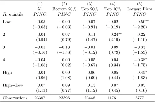
6 AverageP IN C sorted by return quintile . . . 41
7 Market-adjusted annual firm growth rate averages . . . 42
8 Average area growth rate predictability regressions . . . 43
9 Average annual area statistics sorted by prior year P IN C quintile . . . 44
10 Returns sorted onPINC and degree of business localization . . . 45
11 Return predictability conditional on industry-human-capital intensity . . . 46
12 Regression of area returns on PINC and matched PINC . . . 47
13 Return predictability conditional on aggregate house price growth . . . 48
List of Figures
1 U.S. Bureau of Economic Analysis economic areas. . . 31
2 Value of a dollar invested in proprietary income growth portfolio. . . 32
3 Average cumulative return differences. . . 33
4 Average returns for firms located in high versus lowP IN C areas by year. . . . 34
1. Introduction
Silicon Valley was born in 1939, when Bill Hewlett and Dave Packard founded HP in
Packard’s garage with an initial investment of $538. Their first product was an audio oscillator,
and one of their first customers was Walt Disney, who purchased eight oscillators to develop
the sound system for the movie Fantasia. Decades later, in the 1970s, Silicon Valley struggled
against increasing competition from Route 128 in Boston for supremacy in the high technology
industry. Fates diverged, however, and by the late ’80s Silicon Valley was forging ahead as the
global leader in high technology, while Route 128 stagnated.
What caused the divergence in these two local economies? In her comprehensive history
of these two regions, AnnaLee Saxenian (1994) notes that the key difference leading to this
divergent outcome was not resources or location, but that Silicon Valley, true to its roots,
created a culture that fostered entrepreneurship, while Route 128 did not. Today, Silicon
Valley continues to be the center of entrepreneurship and high-tech innovation in the United
States, accounting for more than one-third of its total venture capital.1 This paper explores
the benefits that accrue to public firms from being located near a vibrant entrepreneurial
economy.
Entrepreneurs play an vital role in making regions economically dynamic, in fact,
“en-trepreneurship...is one of the three great predictors of urban success” (Glaesar 2010). Here
I look at the impact of entrepreneurship on public firm outcomes. I find that entrepreneur
performance predicts the performance of neighboring public firms. Specifically, firms
headquar-tered in areas with the highest per proprietor (non-farm) proprietary income growth (hereafter
“proprietary income growth”) have significantly higher abnormal risk-adjusted annual returns
the following year than firms located in areas with the lowest proprietary income growth. This
1
return difference does not reverse, but persists and cumulates over the subsequent 60 months.
Conversely, there is no evidence that firm performance leads local proprietary income growth.
Consistent with evidence that local proprietary income shocks lead real improvements to
neighboring firms, I find that growth in proprietary income also predicts growth in future
investment, R&D, assets, earnings, and cash flows for firms headquartered nearby. In related
research with Parsons and Titman (2012), we find that a firm’s investment co-moves with the
investments of other firms headquartered nearby, even those in very different industries. We
hypothesize that this co-movement is due to time-varying area-specific factors, e.g., investment
opportunities that are positively linked to local business conditions. Consistent with these
findings, I show that in addition to predicting the performance of neighboring public firms,
local proprietary income growth also predicts the performance of the entire local economy, i.e.,
growth in proprietary income predicts future wage growth per employee, future employment
growth, and future growth in the number of proprietors. Moreover, regions in which proprietary
income growth is higher have higher population on average compared to areas with lower
growth, and have significantly more firms per capita— indicating either a higher firm birth
rate or a lower firm death rate.
There are both non-causal and causal reasons to expect that proprietor performance would
forecast changes to its surrounding environment. A non-causal explanation is that proprietor
performance is a leading indicator for the local economy and subsequently for neighboring
public firms. For example, it is possible that, due to simpler operations and centralized decision
making, small entrepreneurial firms are more nimble when adjusting to economic shocks than
their larger, more bureaucratic corporate counterparts.
Alternatively, proprietors could be causally influencing their local economies via their
ef-fect on local entrepreneurship and innovation. Schumpeter (1934) originally theorized that
entrepreneurs were the driving force behind economic growth. Subsequently, multiple studies
have found a strong positive correlation between the number of small, entrepreneurial firms
and subsequent measures of growth (Glaeser et al. 1992; Rosenthal and Strange 2003, 2009;
and Glaeser and Kerr 2009). How might entrepreneurs spur development? One possibility is
and Feldman 2003) which are a commonly-cited motivation for the increasing-returns-to-scale
production critical to endogenous growth theory (Romer 1986, Lucas 1988, and Grossman and
Helpman 1991).2 Giving strength to this idea, Hsu (2011) constructs empirical proxies for
industrial and geographic spillovers using patent data, and finds a positive relation between
spillovers and future firm stock returns and profitability.
To dig deeper into the drivers behind proprietary income growth shocks, I investigate where
proprietary income growth’s predictive ability is strongest. I find that the average difference in
risk-adjusted returns for firms in high growth versus low growth areas increases monotonically
as the sample of firms is restricted to those with more localized business operations. The
average difference for firms with operations in fewer than five states is more than double that
for firms with operations in more than ten states, and completely disappears for firms with
business operations in more than 20 states. Similar attenuation is observed in firm cash flows.
This suggests that whatever is driving local proprietary income growth is predominantlylocal
in nature–i.e., it is probably not due to proprietors’ abilities to respond to aggregate shocks
faster than public firms. Moreover, while this does not rule out a non-causal explanation, it is
consistent with proximity’s significant role in generating knowledge spill-overs.3
Providing further evidence for a spillover-based explanation, I find that this predictability
is strongest in industries where the possession of knowledge plays a prominent role. Using
multiple proxies for industry human capital intensity, I find that the predictability is strongest
for firms in industries with high average patenting, high average wages, and high average R&D.
2
To illustrate, consider the following scenario: When the returns to entrepreneurship are high (e.g., high proprietary income), a worker may choose to exit the firm or university where they work in order to form a new company. (See Lucas 1978, Kihlstrom and Laffont 1979, Holmes and Schmidt 1990, and Jovanovic 1994 for the model of entrepreneurial choice which suggests that individuals choose between earning their income either through employment or through wage work.) However, when employees leave wage work for self-employment, they take with them the knowledge, ideas, and skills from their previous employ. In this way entrepreneurship plays an important function in appropriating knowledge from local firms. However, knowledge transfer isn’t unidirectional. As entrepreneurs retain contacts from their previous job, they spread ideas and knowledge back to the firm. Thus, entrepreneurship stimulates the creation of knowledge networks which subsequently drives economic growth–improving business conditions for surrounding firms.
3
On the other hand, I investigate whether the predictability is due to proprietors responding
faster than public firms to industry shocks. For example, it may be that both proprietors and
public firms in Houston are predominantly oil-industry based firms. Thus, if Houston
propri-etors respond faster than Houston firms to an oil-industry shock, the observed predictability
would be explained. To check this, I classify regions by their dominant industries and then
see if the proprietary income growth rate from another region with the same dominant
in-dustry also predicts returns. For example, I check to see if the proprietary income growth
rate of Portland, an electronics industry hub, predicts Phoenix stock returns—another area
with a dominant electronics industry—the assumption being that a region’s dominant public
firm industry is also its dominant private firm industry. Overall, I find no evidence that the
predictability is due to proprietors’ responding faster than public firms to industry-specific
shocks.
Perhaps the strongest evidence that proprietors causally effect their environment is the
response of future returns to growth in proprietary income, conditional on the relaxing or
tightening of proprietor financial constraints. Research has shown that financial constraints
often dictate entrepreneurs’ decisions to expand their current business or for individuals to
become entrepreneurs.4 Housing prices are particularly important for proprietors in this regard
since they often use housing as collateral for loans (Black, de Meza, Jeffreys 1996). Using
aggregate housing price growth as a proxy for changes in proprietor financial constraints, I
find that conditional on increasing housing prices, i.e., when proprietors are less financially
constrained, the average risk-adjusted annual return for firms in high growth areas over the
return of firms in low-growth areas is more than double the unconditional predictability effect.
On the other hand, the average return difference is close to zero when housing prices are in
decline. This finding is somewhat surprising in the light of previous research, which finds
aggregate housing collateral unconditionally predicts countercyclical returns at both the state
and aggregate level (Kumar and Korniotis 2012; Lustig and van Nieuwerburgh 2005).
4
While this conditional response to proprietary income growth does not imply causality,
it is interesting to note that regardless of what is creating the initial shock to proprietary
income, whether it be driven by proprietors themselves or as the response of proprietors to
outside forces, the positive effects of an increase to proprietary income on public firms only
exist when proprietors have access to financing. Thus, it is not the initial shock which causes
the proprietary income growth that influences firm performance, but rather the response of
the local economy following these shocks.
To summarize, local proprietary income growth predicts firm returns and news about future
firm cash flows. This predictability is strongest for firms whose business operations have a
limited geographic scope, firms in high technology industries, and when proprietor financial
constraints are relaxed. While this does not provide conclusive evidence for either a causal or
non-causal explanation for the predictability, it does suggest that proprietary income shocks are
driven by local technology shocks that propagate to firms via proprietors’ effect on their local
economies. Given these findings, I hypothesize that the observed local return predictability
is due to cash-flow news that is non-diversifiable in local portfolios, e.g., the spillover effects
generated by a new technology within an industry agglomeration. Moreover, as portions of
this non-diversifiable news accumulate at the aggregate level I hypothesize that there will be
a common factor across the local proprietary income growth rates of all regions, which will
pro-cyclically predict aggregate market returns.
Using factor analysis, I find such a factor. This factor explains 54% of local proprietary
income growth rate variation, and predicts aggregate market returns better than the dividend
yield or the consumption wealth ratio, CAY (Lettau and Ludvigson 2001a, b). Interestingly,
this factor is 81% correlated with the proprietary income growth of Silicon Valley, which
itself is a stronger predictor of aggregate market returns than the dividend yield or CAY.
Additionally, both the magnitude and the statistical significance of the predictive ability of
Silicon Valley’s proprietary income growth rate considerably increase conditional on weakening
proprietor financial constraints as measured by aggregate housing prices.
By examining the relationship between proprietor and public firm performance, I build on
the broad impacts on entrepreneurship on urban economies. The best piece of evidence for the
benefits of entrepreneurship on area growth is the strong connection between small average
firm size and subsequent growth (see Glaeser et al., 1992; Rosenthal and Strange, 2003 and
2009). However, as Gleasar, Rosenthal, and Strange (2010) emphasize, this literature has been
limited by the dearth of “exogenous variables that increase entrepreneurship but have no other
impact on the local economy.” My results add to this literature, but run into a similar problem
in establishing causality.
These results also contribute to the literature on stock return predictability. Since stock
prices equal the discounted values of future dividends, predictable variation in returns must
come either from predictable variation in cash flows or predictable variation in discount rates
(see Campbell and Shiller 1988; Campbell 1991). In particular, any variable that forecasts
higher returns must forecast either positive shocks to cash flows, like a positive unexpected
change in firm fundamentals, or negative shocks to discount rates, such as lower future risk
aversion or risk premia.
Typically, predictor variables measure business conditions and consequently posit
counter-cyclical return predictability: high future returns when business conditions are weak, and low
future returns when business conditions are strong (Campbell and Diebold 2009).5 Examples
of such variables include the default spread, term spread, dividend yield (Fama and French
1989), CAY (Lettau and Ludvigson 2001a, b), the ratio of housing wealth to human wealth
(Lustig and van Nieuwerburgh 2005), and the private investment rate (Cochrane 1991). Kumar
and Korniotis (2012) similarly find that U.S. state-level measures of business conditions—a
state’s relative unemployment rate or housing collateral ratio—predict counter-cyclical return
variation in state stock portfolios. Additionally, with the exception of CAY, there is little
evidence that any of these variables predict firm cash flows (Menzly, Santos, and Veronesi 2004,
Cochrane 2008, Vuolteenaho 2002). Consequently, research has overwhelmingly attributed
stock return predictability entirely to time-varying discount rates and not predictable cash
5
flow news (Cochrane 2010).6
However, there are exceptions to this rule. Variables that predict technology or productivity
shocks, i.e., systematic cash-flow shocks, are positively correlated with future returns and firm
profitability. These variables include firm productivity (Cochrane 1991, 1996; Liu, Whited,
and Zhang 2009, Balvers and Huang 2007), government investment in public sector physical
capital (Belo and Yu 2012), aggregate patenting and R&D (Hsu 2009), proxies for industry
and geographic knowledge spillovers (Hsu 2011), and various measures of R&D intensity (See
Chan, Lakonishok, and Sougiannis 2001; Lev and Sougiannis (1996); Eberhart et al. 2004;
Hirshleifer et al. 2010). Similar to these variables, growth in proprietary income growth
behaves most like a technology or productivity shock since it predicts pro-cyclical returns and
future firm fundamentals, with the majority of its predictive power being limited to firms in
high technology industries.
At their most basic level, my findings provide evidence that the performance of small
private firms leads the performance of larger public firms located nearby. However, viewed
more expansively, these results highlight the powerful effect a small minority of innovative
entrepreneurs can have on both local and aggregate firm performance—with a special emphasis
on the role Silicon Valley technological innovation has played over the past 40 years in driving
aggregate stock market performance.
The remainder of the paper is set up as follows: Section II describes the data and
method-ology used throughout the paper. Section III reports stock return and firm fundamental
predictability results. Section IV reviews stock return predictability conditional on firms
hav-ing localized business operations, by industry human-capital intensity, and conditional on
changes in aggregate housing collateral. Section V examines local proprietary income’s ability
to predict the aggregate stock market, and Section VI concludes.
6
2. Data description and summary statistics
The data used in this paper consists of all public companies listed on the NYSE,
NAS-DAQ, or AMEX between January 1970 and December 2009. For each of these firms, I obtain
monthly common stock returns from CRSP, and annual firm fundamental data and firm
head-quarter location (ADDZIP) from the CRSP/COMPUSTAT Merged Database. To minimize
the influence of outliers all firm stock returns and fundamental data are winsorized at the one
percent level. Financial firms and regulated utility firms are dropped from the sample.
The economic region of interest is the Economic Area, hereafter EA, as defined by the
United States Bureau of Economic Analysis (BEA). The United States consists of 179 mutually
exclusive and collectively exhaustive EAs. Figure 1 shows a map delineating these regions.
An EA is defined as “the relevant regional markets surrounding metropolitan or micropolitan
statistical areas,” and are “mainly determined by labor commuting patterns that delineate
local labor markets and that also serve as proxies for local markets where businesses in the
areas sell their products.”7 EAs are chosen as the geographic unit of observation since they
are defined according to labor market boundaries. There is little research as to how far
knowledge spill-overs spread; however, focusing on regional labor markets as opposed to cities
seems reasonable given that many industry agglomerations, for example Silicon Valley or the
Research Triangle in North Carolina, span multiple cities.
Firm location is determined by the residence of their corporate headquarters. Firms are
matched to EAs using their headquarter zip code listed on COMPUSTAT. Of course,
head-quarter location is only a rough proxy for firm location, since firms typically have operations
in multiple areas. To address this problem, I follow Garc´ıa and Norli (2012) and use
state-name counts from firms’ annual 10-K statements to measure the geographic scope of a firm’s
operations.8 Firm 10-K statements typically list information on the firm’s properties, such as
factories, warehouses, and sales offices. For example, a firm may include sales by the state
in which they are operating stores, or list their manufacturing facilities by location. Thus,
7
Seehttp://www.bea.gov/regional/docs/econlist.cfm.
state-name counts provide a reasonable proxy for the degree of firm localization. Firms that
do not mention any U.S. state names in their 10-K are excluded from the sample. Due to data
availability, state-name counts are only available for the 12-year period from 1996 to 2008.9
During this period, firms with non-zero state-name counts make up approximately 80% of
firms in the sample each year. This sub-sample is particularly important for my results, since
firms with operations in fewer states are probably more closely tied to their local economy,
and hence more effected by changes in local proprietary income growth.
The variable of primary interest is the demeaned annual per proprietor (non-farm)
propri-etary income growth rate, denoted hereafter as P IN C. This variable is calculated as follows
Proprietary income growtha,t= log
Proprietary income
a,t
No. of proprietorsa,t
−log
Proprietary income
a,t−1
No. of proprietorsa,t−1
P IN Ca,t= Proprietary income growtha,t−
1 179
179 X
a=1
Proprietary income growtha,t
whereadenotes geographic area–either EA or state,tdenotes the year, and1791 P179
a=1Proprietary
income growtha,t is the average proprietary income growth rate across all EAs in year t.
De-meaning adjusts for aggregate fluctuations in proprietary income, so that P IN C is a purely
local measure of proprietary income variation.10 Proprietary income consists of the excess
revenue over explicit production cost of owner-operated businesses (e.g., sole proprietorships,
partnerships, and tax-exempt cooperatives), and is equal to slightly less than 10% of national
income. Data used to construct P IN C as well as area population, employment, and wage
data are obtained from the BEA and begin in 1970.
Essentially,P IN C is a proxy for the time-varying returns to entrepreneurship in an area—
that is, it is the average amount an individual can expect to earn by becoming a proprietor
9
Some 10-K state-name counts are available for 1994 and 1995, however, the sample of firms for these years is small averaging only 22% of stocks in the sample for those years. Consequently, these years are excluded from this sub-sample.
10It is interesting to note that average proprietary income growth is also a weak predictor of stock
at any given time. Many ways have been suggested to measure entrepreneurship—typical
measures include the number of proprietors or small businesses per area, however, these
mea-sures often follow, rather than lead, changes in proprietary income. For example, a high
number of proprietors in an area does not cause average proprietor income to rise nearly as
much as an increase in average proprietor income causes individuals to become entrepreneurs.
Glaeser, Rosenthal, and Strange (2009) state that the five facets of entrepreneurship are
self-employment, small firms, ownership, entry, and innovation. While the number of entrepreneurs
or the number of small firms captures the first four aspects of entrepreneurship, they fail to
capture the time-varying effects of entrepreneur innovation. I hypothesize thatP IN C is a
sig-nificantly better measure in this regard since it provides a direct measure of the profitability
of entrepreneurs in an area.
The distribution of proprietors by skill-level typically follows a U-shape pattern: the
num-ber of proprietors in an area is high for both less educated, low-income individuals and
high-income, well-educated individuals. One short-coming of BEA proprietary income data is that
it is not industry specific. Thus, identifying who the proprietors are that make up the sample
is difficult. For example, I can’t distinguish in the data whether income growth is driven by
hot-dog vendors or high-tech startups.11 However, I conjecture that any sizeable growth in
P IN C will be driven primarily by innovations from high-value entrepreneurs. This conjecture
is consistent with my finding that P IN C primarily predicts returns for firms in innovative,
high human-capital industries.
Since stock return anomalies often exist primarily in stocks with small market
capitaliza-tion, to minimize the effect of these firms on results, firms in the smallest quintile of market
capitalization at the beginning of each year are dropped from the sample. Newly listed firms
are also dropped by this filter since they have no market capitalization in the previous year. To
diminish the possibility of reverse causality—for example, a single firm that drives an area’s
11
entire local economy including P IN C—any areas containing firms consisting of more than
50% of the area market capitalization are dropped from the sample. Typically this filter drops
rural areas with only one or two firms from the sample. Including micro-caps and high area
market-share firms does not change my results, other than slightly inflating the size of the
over-all return predictability. To additionover-ally reduce the effect of size, portfolios are value-weighted
by firms’ previous year market capitalization.
All annual variables are in real terms and are deflated using CPI data from the Bureau
of Labor Statistics. All growth rates and returns are in percentages. Additional data used
includes firm-specific patenting data from the NBER patent database for patents granted
between 1976 and 2006, annual and monthly Fama-French factor data obtained from Ken
French, and monthly DGTW returns for the years 1975-2009 obtained from Russ Wermers.12
DGTW benchmark portfolios prior to July 1975 are constructed by the author. Housing price
data and housing collateral data is obtained from Robert Shiller13and Stijn Van Nieuwerburgh
14, while data from the Federal Reserve Board’s “Senior loan officer opinion survey on bank
lending practices” 15 is also used. CAY data is obtained from Martin Lettau16, and
payout-adjusted dividend yield data is obtained from Michael Roberts17.
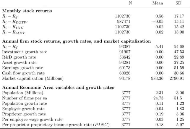
Summary statistics for the majority of variables used are recorded in Table 1. This table
reports the mean and standard deviation for monthly excess and risk-adjusted stock returns;
annual stock returns, firm fundamental growth rates, and firm size; and EA-specific variables
such as population per EA, number of firms per EA, etc. Growth rates are demeaned annually.
EA growth rate averages deviate slightly from zero since the table summarizes only growth
rates for areas with a non-zero number of public firms, while demeaning uses information from
12The Fama-French factor data are available via http://mba.tuck.dartmouth.edu/pages/faculty/ken.
french/data_library.html. The DGTW benchmarks are available viahttp://www.smith.umd.edu/faculty/ rwermers/ftpsite/Dgtw/coverpage.htm
13
http://www.econ.yale.edu/~shiller/data.htm
14
http://pages.stern.nyu.edu/~svnieuwe/
15
http://www.federalreserve.gov/boarddocs/snloansurvey/201201/chartdata.htm
16
http://faculty.haas.berkeley.edu/lettau/data.html
17
all EAs.
Table 2 reports the probability of an EA transitioning from oneP IN Cquintile this year to
anotherP IN C quintile the following year. Interestingly, the probability distribution appears
to be flat. Moreover, the average P IN C autocorrelation across EAs is 0.034. This lack of
persistence in P IN C is due, somewhat, to increases in the number of proprietors following
growth in P IN C, but, more importantly, to the nature of P IN C’s variation. Namely, the
highly-stochastic nature ofP IN Cis consistent with my hypothesis that changes to this variable
are driven primarily by innovations from high-value entrepreneurs.
3. P IN C predicts returns and news about future cash flows
My primary empirical results show that growth in proprietary income per proprietor
(P IN C) predicts firm stock returns and fundamental growth rates. For example, Figure 2
shows the value of a dollar invested in the beginning of 1972 in a value-weighted portfolio of
all firms in the sample that year (the market portfolio) and value-weighted portfolios
consist-ing of firms located in EAs in the top and bottom quintiles of P IN C in the previous year.18
At the end of 2009, the strategy of investing in the high growth portfolio each year is worth
$9.71—almost twice the return on the market portfolio ($5.58) and roughly four times the
amount earned investing in firms located in low growth areas ($2.64).
In Section 3.1, I examine P IN C’s ability to predict returns both cross-sectionally and
across time. First, I look at monthly risk-adjusted stock returns sorted by prior year P IN C
quintile. Next, I examine P IN C’s ability to predict returns though time by forming
value-weighted area portfolios consisting of all stocks in an EA and then running panel predictive
regressions of EA portfolio returns on lagged P IN C. In both cases, I find that P IN C is a
strong predictor of future returns. I also check for evidence of reversal or reverse causality, but
find none.
In addition to returns, Section 3.2 reports evidence thatP IN C predicts news about future
18
firm cash flows. I find that P IN C predicts growth in firm investment, R&D, assets, earnings
and cash flows. As with returns, this predictability exists both in the cross-section and time
series. Finally, in Section 3.3, I examine P IN C’s effect on its local economy, and report area
characteristics by average P IN C quintile.
3.1. Risk-adjusted return predictability
Tables 3 and 4 present average risk-adjusted monthly stock returns for firms according to
the performance of proprietors where firms are headquartered in the previous year. Specifically,
each year, economic areas are ranked byP IN C. Based on this ranking, firms are sorted into
quintiles. In Table 3, equal-weighted return averages are then taken across time and firms,
while in Table 4 value-weighted portfolios are formed by P IN C quintile and Fama-French 4
factor regressions are run.
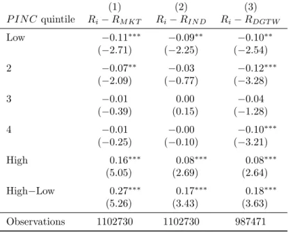
In the first column of Table 3, returns are market-adjusted by the value-weighted monthly
average of all returns in the sample. A quick inspection shows a strong monotonic pattern
between last year’s proprietary income growth rate and this year’s market-adjusted stock
returns. On average, firms headquartered in areas with the highest P IN C quintile in the
previous year experience monthly market-adjusted returns which are 27 basis points bigger, or
3.24% annualized (t-statistic = 5.26), than firms headquartered in areas with the lowest quintile
ofP IN C. Similar patterns exist for industry-adjusted and DGTW-adjusted returns. Column
2 shows results for returns adjusted monthly by their corresponding value-weighted
Fama-French 49 industry portfolio return. The average difference between firms in high- and
low-growth areas is 17 basis points per month, or 2.04% annualized (t-statistic = 3.43). Column 3
adjusts returns by their characteristic-matched DGTW benchmark, i.e., a benchmark portfolio
matched to firm’s by their prior year size, book-to-market and momentum characteristics.19
Similar to the industry-adjusted return results, the average difference between firms in
high-and low- growth areas is 18 basis points per month, or 2.16% annualized (t-statistic = 3.63).
Table 4 reports Fama-French 4-factor regression results. Value-weighted portfolios are
19For more information on how DGTW benchmarks are constructed, see Daniel, Grinblatt, Titman, and
formed according to firms’ previous yearP IN C quintile and portfolio returns are regressed on
the three Fama-French (1993) factors: the excess return on the market portfolio, MKTRF; the
small-minus-big portfolio return, SMB; and the high-minus-low portfolio return, HML; and the
Carhart (1997) momentum factor, MOM.20 Each row in the table corresponds to a different
quintile portfolio. The last row reports regression results for a portfolio that is long firms in
the highest P IN C quintile the previous year and short firms in the lowest P IN C quintile.
Similar to Table 3 results, the long-short abnormal return (ALPHA) is 36 basis points per
month, or 4.32% annualized (tstatistic = 2.64). This return is slightly larger than those found
in Table 3, due to an extreme outlier in 1971. Excluding returns in this year the long-short
abnormal return is 22 basis points (t statistic 1.83), or 2.64% annualized. Thus, it can be
concluded that the average risk-adjusted return difference for firms in high growth versus low
growth areas is a robust, statistically-significant 2% per year over the 39-year sample period.
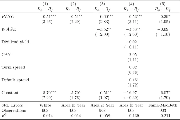
Table 5 shows pooled panel regressions of excess area portfolio returns on lagged P IN C
and other controls. Specifically, it reports results for the following regression
Ra,t−Rf,t=α+βP IN Ca,t−1+γW AGEa,t−1+η·Xt−1+εa,t (1)
where Ra,t is the annual return on a value-weighted portfolio consisting of all firms in EA
a at year t, W AGEa,t−1 is the per employee wage growth rate by EA, and X is a vector
of known predictor variables: the aggregate payout-adjusted log dividend yield,21 CAY, the
term spread, and the default spread. Regression results are presented for a variety of standard
error estimation schemes. Additionally, to diminish the possibility of extreme portfolio returns
from under-diversified portfolios, area portfolios are required to have at least 20 firms in the
previous year to be included in the sample.
The first two columns of Table 5 include only P IN C as a regressor. The coefficient in
this case is 0.52 for OLS regressions. The standard deviation of P IN C for this sub-sample
20I also looked at five factor regressions including the Pastor-Stambaugh liquidity factor. However this
variable was statistically insignificant in all regressions so I have excluded it.
is 5.36, hence, a one-standard deviation increase in an area’s P IN C would imply a 2.79%
increase in average area returns next year. In the first column, White standard errors are
reported, and in second column standard errors are calculated clustering on both area and
year. In unreported results, I find that the standard errors clustered by area are only slightly
smaller than the White standard errors, and that the standard errors from double-clustering
are almost identical to the standard errors obtained by clustering on year. Essentially, this
implies that that area effects are small in this regression (e.g., return autocorrelation does not
seem to be much of a concern), while adjusting standard errors to correct for co-movement of
area portfolios within a year is paramount to obtaining correct standard error estimates.
In Column 3, W AGEis added as a regressor. Adding this variable increases the coefficient
on P IN C by about 18%, which suggests that P IN C is measuring more than simply
fluctua-tions in local business cycles. Similar to other area-level predictor variables (see Kumar and
Korniotis, 2012),W AGE predicts counter-cyclical return variation. Additional variables that
have been shown to predict aggregate market returns are added as regressors in Column 4,
although only the default spread is close to being statistically significant. In the last column,
I verify my estimates by estimating equation (1) using a MacBeth regression.
Fama-MacBeth regressions are designed to adjust for cross-sectional correlation within a panel. The
P IN C coefficient estimate and associated t-statistic are near their OLS counterparts
clus-tered on area and year. However, the coefficient onW AGE is much smaller and subsequently
W AGE is no longer a statistically significant regressor.
One possible explanation for the observed predictability is that it is due to reverse causality.
For example, it could be the case that public firms and proprietors do well contemporaneously
and that subsequent return momentum generates the observed results. To test this, I sort
returns into quintiles each year and examine the average P IN C by return quintile. Table 6
reports these results. Column 1 shows results sorting on the full sample of returns. Column
2 reports results sorting on only firms in the second quintile of market capitalization. This
column tests for the possibility that growth in proprietor income is correlated to factors that
drive small firm returns. Perhaps the most reasonable case for reverse causality is a dominant
using only firms in the largest market capitalization quintile, the largest market capitalization
decile, and the return of the firm with the largest market capitalization in each area. In none of
these sorts do I find any evidence that returns are contemporaneously correlated withP IN C.
Additionally, in unreported results, I check to see if firm returns predict P IN C: Firms are
sorted into quintiles by their current returns and averages are taken of their corresponding
P IN C next year. Similar to results using contemporaneous returns and P IN C, I find no
evidence of reverse causality.
Another possible explanation for the observed predictability is investor overreaction. If this
were the case then I would expect returns to reverse in the future as arbitrageurs correct asset
prices. Figure 3 shows a plot of the average cumulative returns of a value-weighted portfolio
that is long firms with high P IN C in the sorting year and short firms in the lowest P IN C
quintile. The plot shows cumulative raw returns (dashed line) and cumulative DGTW-adjusted
returns (solid-line) for 60 months before the sorting year, the 12 months during the sorting
year, and the 60 months after the sorting year. Since five years are required to construct
averages, the data used to construct this plot are from 1976 to 2004. Both during the sorting
year and in the 60 months before the sorting, there appears to be no run-up in cumulative
returns, consistent with the results of Table 6 which find no evidence of reverse causality. In
the first year following the sorting, average cumulative returns increase by approximately 3%.
Cumulative returns continue to rise over the following 48 months, and show no sign of reversing.
Thus, I conclude that there is little evidence for a story involving investor overreaction.
3.2. Cash flow predictability
To be consistent with a lack of reversal and pro-cyclical return predictability, I should also
find that P IN C predicts firm fundamental growth rates. Table 7 reports average
market-adjusted firm fundamental growth rates by prior year P IN C quintile. Growth rates are
calculated as log differences, hence negative earnings and cash flows are dropped.22 Column
22There are several reasons why firms have negative earnings. Typically these reasons can be classified as
1 reports average investment growth rates byP IN C quintiles, Column 2 R&D growth rates,
Column 3 asset growth rates, Column 4 earnings growth rates and Column 5 cash flow growth
rates. For each of these measures, growth rates are roughly 1% higher per year following high
P IN C versus following lowP IN C in an area. In particular,P IN C is cross-sectionally a very
strong predictor of firm investment and R&D growth rates.
Examining P IN C’s ability to predict fundamental growth rates through time,
value-weighted growth rate averages are taken by area, ga,t, then the following pooled-panel
re-gressions are run for each fundamental growth rate:
ga,t=α+βP IN Ca,t−1+εa,t (2)
Standard errors are clustered on year and area, and regression results are reported in Table
8. As with Table 7 sorts, the results in Table 8 suggest that P IN C is strongest predicting
growth in investment and R&D. However, some evidence also remains that P IN C predicts
asset and cash flow growth rates.23 The standard deviation ofP IN C for this sample is 5.36.
Thus, a one-standard deviation increaseP IN Cincreases investment by 1.13%, R&D by 0.43%,
assets, 0.64%, and cash flows by 0.59%. Both cash flow and asset growth rates are statistically
significant at the 10% level, while investment and R&D growth rates are statistically significant
at the 5% level.
3.3. P IN C as a measure of area vibrancy
How are areas where P IN C is consistently high different from areas where P IN C is
consistently low? Table 9 answers this question. In this table, firms are sorted according to
prior year P IN C and annually-demeaned averages of area variables by P IN C quintile are
reported. P IN C is correlated with area population: areas with higher P IN C on average,
have about 310,000 more people, on average, than those with low P IN C. This difference is
earnings, however, the interpretation of these variables is difficult.
23Of course, fundamental predictability should be weaker than stock return predictability, as stock returns
statistically significant at the 10% level, however this is not a huge difference given that the
average area population is roughly 2.3 million people. There is not a significant difference in
the average size of firms in high growth versus low growth areas. However, high growth areas,
on average, have about 1.09 more firms per capita than low growth areas. The difference in the
number of firms per capita is statistically significant at the 1% level. This finding is interesting
since it says that either the birth-rate of new firms is higher, or the death-rate of firms is lower in
areas whereP IN Cis consistently high versus areas whereP IN Cis consistently low. Whether
this is caused byP IN C or is also determined by other factors is unknown, and is left for future
investigation. However, this finding implies interesting possibilities for P IN C as a proxy for
the time-varying health of an area. This is not surprising, though, given entrepreneurship’s
key role in generating urban success.
In addition to affecting nearby public firms, it is possible that P IN C is also correlated
with changes in the local economy. That is, regardless of whether P IN C is causing changes
in public firms or merely reacting faster to common shocks, it is informative to see whether
P IN Calso leads its local economy. Columns 4 through 6 look at the average proprietor growth
rate, employment growth rate, and per employee wage growth rate by prior year’s P IN C,
respectively. P IN C is a strong predictor of future proprietor, employment, and per employee
wage growth. Thus, when proprietor income in an area rises, the number of proprietors in
the following year increases, as do the number of employed workers and the average wage
per employee. Unfortunately, I cannot tell whether the increase in employees and wages is
driven by the successful proprietors hiring more individuals and paying them higher wages, or
whether this is simply an improvement similar to the one experienced by proprietors in the
previous year. Overall, it appears that, on average, areas with high levels of proprietor success
are economically more successful than areas with lowP IN C.
4. Conditional P IN C predictability
In this section, I further examine the established predictive ability of P IN C. Here, I hope
that P IN C is strongest when predicting changes in local firms, in firms in
human-capital-intensive industries, and following the weakening of proprietor financial constraints. I also try
to determine whether the observed predictability is due to proprietors’ abilities to respond
more quickly to industry shocks, but find little evidence for this story. Given my findings,
I conclude that the shocks driving P IN C are local in nature and likely due to technology
shocks. I also find that the transmission of these shocks to public firms is deeply intertwined
with proprietors’ abilities to respond to fluctuations inP IN C.
4.1. Predictability conditional on firm localization
If the observed predictability patterns are due to local factors, my results should be stronger
when limiting firms to only those with localized operations. Table 10 shows that this is,
indeed, the case. Similar to Garc´ıa and Norli (2012), I use state-name counts from firms’
annual 10-K statements as a proxy for the geographic scope of a firm’s operations. Panel
A of Table 10 reports the average monthly DGTW-adjusted return for firms by prior year
P IN C quintile and degree of firm localization as determined by prior year state-name counts.
Because state-name counts are only available for a sub-sample of years, Column 1 of this
table reports average returns for the full sub-sample period (1996 - 2008) for which state-name
count data is available. Similar to results calculated using the full sample, I find thatP IN C
leads returns, however, over this time period, the correlation between P IN C and returns is
much stronger and generates a risk-adjusted return difference of 64 basis points per month, or
7.68% annualized (t-statistic = 6.13), between firms in high- and low-growth areas. Columns
2 through 5 report the same results as Column 1 limiting the sample to only firms that have
operations in one state (Column 2), only firms that have operations in five or fewer states
(Column 3), only firms that have operations six to ten states (Column 4), and only firms with
operations in more then ten states (Column 5). Consistent with my hypothesis thattruly local
firms will be more affected by proprietary income shocks, I find that the relationship between
growth and returns is stronger for more-localized firms with a very strong monotonic pattern
for firms located in the highest P IN C quintile in the previous year. The average
one state to four basis points for firms with operations in more than ten states.
Since returns are DGTW-adjusted, the fact that localized firms are likely also smaller firms
does not imply that these results are being driven by a “small firm” effect—i.e., these results
are not due to simply sorting on firm size. However, it is informative to further sort the sample
on firm size, to see if P IN C affects small firms disproportionately more than large firms. In
unreported results, I sort firms into size quintiles and then look at firms in the smallest size
quintile with operations in five or fewer states. The average return difference for small firms
located in high- versus low-growth areas is 1.18% per month, or about double the difference
for firms in the largest size quintile, in which case the difference is about 66 basis points per
month. Interesting, though, is the asymmetric response of big and small firms to high and low
proprietary income growth. Big firms are much more negatively affected by low P IN C than
small firms, while small firms tend to benefit much more from high P IN C than big firms.
My hypothesis is that highP IN C is an indicator for future growth opportunities which small
firms can capitalize on while large firms, which are largely set in their ways, cannot.
4.2. Predictability conditional on industry human-capital intensity
To further understand the shocks driving changes in proprietary income growth and returns,
I examine P IN C’s ability to predict returns conditional on firm’s industry human-capital
intensity, as defined by their Fama-French 49 industry classification. To measure industry
human-capital intensity, I calculate value-weighted averages by industry for the number of
patents per firm (log(1 + Number patents per firm)), the average Selling, General and
Admin-istrative Expenses (SG&A) per employee per firm (log(1 + SG&A/Employees)), where SG&A
is used as a proxy for firm wages, and the average R&D per firm (log(1 + R&D)). The idea
be-ing that firms in high human-capital industries produce more innovations, earn higher wages,
and conduct more research. Industry average patenting is 36% correlated with both industry
average wages per employee and industry average R&D, while industry average R&D and wage
Table 11 reports regression results for the following equation:
Ri,I,t−Rf,t=α+βP IN Ca,t−1+ζP IN Ca,t−1×Human CapitalI,t−1+γHuman CapitalI,t−1+εa,t
(3)
where Ri,I,t is the return of firm iin industry I at time t,Human CapitalI,t−1 is one of the
above mentioned industry human-capital-intensity proxies. Standard errors are clustered on
year and firm. To diminish the effect of outliers, I require that there be at least five firms per
industry within an area in the previous year to be included in the sample.
I am primarily interested in the interaction between industry human-capital intensity and
P IN C. I find that this interaction is statistically significant at the 5% level for industry
average patents and industry average wages, and statistically significant at the 10% for industry
average R&D. For example, a one-standard deviation increase in industry patenting (standard
deviation = 0.51) increases the coefficient on P IN C to 0.58, which is similar to the P IN C
coefficient found in Table 5. Overall, these results imply that the predictive capability of
P IN C resides mainly in its ability to predict the returns of firms in high human-capital,
i.e., high technology industries. While certainly not conclusive evidence, these findings are
consistent with P IN C’s predictive abilities being connected with knowledge spillovers. I run
similar regressions for cash flow growth, but find no statistically significant interactions, so
results are not reported.
Due to P IN C’s strong interaction with industry-related factors, I hypothesize that its
predictive ability may be due to proprietors responding faster than public firms to common
industry shocks. This could be the case if both the local public and private sectors shared
a common industry concentration–something which is likely for areas with strong industry
agglomerations, such as Silicon Valley or Detroit. To examine this possibility, I run
time-series regressions of value-weighted annual area portfolio returns on the laggedP IN C from an
area with a similar industry concentration. If P IN C and returns are being driven by shared
industry shocks, then theP IN Cfrom another area with similar industry-concentrations should
also be able to predict area returns.
of proprietary income data is that I cannot separate proprietors by industries. Thus, to
determine an area’s dominant industry, I must rely solely on measures constructed from public
firm data. I define an industry as dominant if it has the largest industry market share within
a given area, and an area as having a dominate industry if, for more than 40% of the years
it is in the sample, it has the same dominant industry. For example, I find that from 1970 to
2009 the oil industry has had the largest industry market share for Houston 39 out of its 39
years in the sample. Thus, I define Houston’s dominant industry as oil.
Using these area-industry classifications, I match areas to those with a similar dominant
industry. If an area has more than one matched area with the same dominant industry,
then the matched-area with the the highest percentage of dominance is considered that area’s
“Matched P IN C.” For example, New York City, Atlanta, and Washington D.C. are each
considered dominant in the business services industry (Fama-French industry classification
#34). When looking for an area-industry matched pair for Washington, D.C., both New York
City and Atlanta will work. New York City is chosen because it is dominated by business
services 85% of the time while Washington, D.C. is dominated by business services only 50%
of the time.
Table 12 reports regression results for this test. To be included in the sample, I require
each area to have at least 20 years of observations with at least 20 firms in the previous year,
and to have a matched area/industry. The 20 firm requirement is to ensure that portfolios
are reasonably well diversified, and the 20 years requirement is so I have enough data to run
time-series regressions. These filters decrease the sample to 13 economic areas. Each row of
Table 12 represents regressions for a different economic area. Since the table is somewhat
complex, I begin by explaining the results for a single area Atlanta (EA 11) in the first row.
The first column reports the economic area of interest, and the second and third columns its
dominant industry with the corresponding percentage of years this industry dominates. For
example, Atlanta’s dominant industry is Business Services which is dominant 59% of the 37
years Atlanta is in the sample. The fourth column reports the area’s matched industry-area
pair. For Atlanta this match is EA 118–New York City.
returns on laggedP IN C. For example, in the first row, results are reported for a regression of
Atlanta portfolio returns on Atlanta’sP IN Cfrom the previous year and a constant. There are
37 observations in this regression and the coefficient on P IN C is a statistically insignificant
-0.35. It is interesting to note the areas for whichP IN C is a strong predictor of area returns:
Overall, P IN C is statistically significant at the 10% level or better in 5 of the 13 areas in the
sample. As expected from the results in Table 11, the majority of the predictability comes
from areas where the dominant industry is human-capital intensive (e.g. Phoenix, Portland,
and San Jose). Detroit interestingly has a negative correlation with P IN C, suggesting that
the performance of public firms is being crowded out by the entrepreneurial sector following a
rise in entrepreneur incentives.
In the final column I report results for time-series regressions of area portfolio annual
returns on the lagged matched areaP IN C. If common industry shocks are driving the
corre-lations between currentP IN C and future returns, then MatchedP IN C may also be able to
predict future area returns. In examining these regressions, I find no evidence that this is the
case, as none of the matchedP IN C coefficients are statistically significant. Combining these
results with those conditioning on firm localization, I conclude that whatever is driving the
correlations betweenP IN C and returns is most likely not aggregate-market or industry-level
shocks, but rather shocks originating within the local area.
4.3. Predictability conditional on financial constraints
Financial constraints are a key concern to proprietors. Moreover, since proprietary
busi-ness’s are often small, proprietors often use their homes as loan collateral to obtain financing
for future investments.24 This makes housing prices an important component of their
invest-ment decisions. If proprietors are the channel through which proprietary income growth shocks
are propagated to public firms, then the magnitude of their effect on public firms and
subse-quently the degree of predictability, should increase when housing prices are on the rise. To
24For example, small business’ owners often finance operations with a second mortgage on their home (also
test this hypothesis, I examine P IN C’s predictive ability conditional on whether aggregate
housing prices or housing collateral were rising during theP IN C sorting year.
I use two proxies to measure changes in aggregate housing collateral: The first is the
growth rate (log difference) of the ratio of collateralizable housing wealth to non-collateralizable
human wealth (from Lustig and Van Nieuwerburgh 2005), where the housing collateral stock
is measured by the market value of residential real estate wealth.25 I call this variable housing
collateral growth. Since this time series only goes to 2002, I also use the growth rate (log
difference) of the annual real home price index for the U.S. The housing collateral growth rate
and housing price growth rate are 59% correlated, and sorting on either rate produces very
similar results.
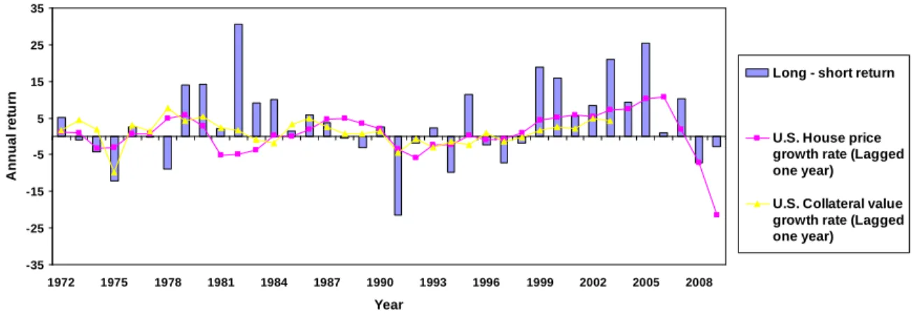
Panel A of Figure 4 plots the yearly difference in the value-weighted portfolio return of all
firms located in the highestP IN Cquintile areas in the previous year minus the value-weighted
portfolio return of all firms in the lowestP IN C quintile.26 On top of this is also graphed the
time-series of U.S. home price growth lagged one year, and the housing collateral growth rate
time-series lagged one year. From this plot, it is simple to see the strong correlation between
both housing collateral and housing price growth rates. Additionally, a cursory inspection
reveals the negative correlation between housing collateral and price growth rates and the
long-shortP IN C quintile portfolio. Panel B plots a similar figure, except that in years when
the lagged housing price rate is less then zero, it plots the difference between low growth
quintile portfolio minus the high growth quintile portfolio. Doing this decreases the number of
years in the sample with negative returns less than -5% from six to three, with a substantial
improvement in the latter half of the sample. This is somewhat surprising given that Lustig and
Van Nieuwerburgh (2005) find that higher housing collateral growth unconditionally implies
negative aggregate returns. Thus, it is the interaction of housing price changes with proprietor
income growth that causes the changes in firm returns and not the changes in housing prices
25
Lustig and Van Nieuwerburgh (2005)also use the value of outstanding home mortgages and the net stock current cost value of owner-occupied and tenant-occupied residential fixed assets as measures of aggregate housing collateral stock. Using these alternative measures to calculate housing collateral growth yields very similar results to using the market value of residential real estate wealth.
26
alone.
To formalize these visual observations, Table 13 reports DGTW-adjusted monthly returns
for firms sorted according to their prior year’sP IN C, conditional on whether housing collateral
or prices rose or fell over the prior year. The first column shows that, conditional on aggregate
housing prices rising during the sorting year, the average DGTW-adjusted return for firms
located in areas with high proprietary income growth in the prior year is 40 basis points (4.8%
annualized) over the average DGTW-adjusted return for firms located in areas in the lowest
quintile of proprietary income growth in the prior year. This value is statistically significant
at the 1% level. Interestingly, this pattern reverses when housing prices are decreasing and
financial constraints are tightening during the sorting year. In this instance, the average
difference between firms in high and low growth areas is -15 basis points (-1.8% annualized).
Thus, conditioning on weakening financial constraints for proprietors more than doubles the
magnitude of the predictability.
To verify the results using housing price growth rates, I also report results sorting on
housing collateral growth rates and mortgage loan survey data. Columns 3 and 4 find similar
results sorting on growth in aggregate housing collateral: in years following housing collateral
increases, the long-short return is 42 basis points, and in years following house price decreases,
the long-short portfolio is -24 basis points.
One peculiarity is the negative correlation between P IN C and returns conditional on
falling housing prices. A possible explanation for this is that housing collateral growth is also
a proxy for aggregate business cycles. In this sense, if the aggregate economy is in a recession
and local proprietors are doing well, the incentives to become proprietors may be stronger than
otherwise. Subsequently high proprietor growth during downturns substantially hurts public
firms as talented workers leave wage work for self-employment.
In sum, these results do not necessarily imply that local proprietors are causally effecting
neighboring public firms. However, given that the return predictability is only positive when
housing prices are also rising, i.e. only when proprietor financial constraints are weakening,
does suggest that even if proprietors are not the immediate cause for firm stock prices changing,
it is not merely the increase in proprietor income that leads to higher firm returns, but the
local economy’s response after that shock that determines how firms internalize the success of
proprietors.
5. Aggregate market return predictability
In the previous section, I showed that P IN C’s predictive ability was strongest for firms
with localized business operations and for firms in human-capital-intensive industries.
Addi-tionally, I showed that the state of individuals’ financial constraints had a way of magnifying
or diminishing the effect of these shocks within the local economy and, ultimately, to public
firms.
Given this evidence, it appears that growth in local proprietary income is most likely
gen-erated by a technology or productivity shock for three main reasons: First, similar to other
measures of technology shocks (such as aggregate patenting or R&D) and unlike typical
mea-sures of business conditions (such as CAY or the dividend yield), local proprietary income
growth predicts pro-cyclical stock returns, i.e., high local proprietary income growth is
fol-lowed by higher returns, and low growth by low returns. Second, return predictability due to
proprietary income growth rates is concentrated primarily in high-human-capital industries,
where innovations are paramount and technologies are constantly changing. Finally, growth in
local proprietary income predicts growth in the future investment, R&D, earnings, and cash
flows for firms headquartered locally, consistent withP IN C being correlated with predicable
variation in news about future cash-flows.
Typically cash flow news does not matter for return predictability because it is highly
id-iosyncratic and subsequently, diversifies away in large enough portfolios (Vuolteenaho, 2002).
However, it is simple enough to think of systematic cash-flow news: for example, a new
tech-nology within an industry agglomeration. In the case of the above predictability patterns,
it appears that P IN C is predicting news about local cash flows that is non-diversifiable in
local portfolios. I hypothesize that, since these cash flow shocks do not diversify out in local
portfolios, some of these shocks will not diversify out in aggregate portfolios either.
EAs, and test for a common factor that prices returns across all areas and subsequently the
aggregate stock market. Doing precisely this, I find such a factor. This factor explains roughly
54% of the variation across all P IN C time series. Column 1 of Table 14 reports the results
for a regression of the CRSP value-weighted market portfolio excess return on a one-year lag
of this factor. The coefficient on the lagged factor is 6.89 (t-statistic = 2.98), which, since
the factor has a standard deviation of 1 by construction, implies an increase in the aggregate
market return of 6.89% following a one-standard-deviation increase in this factor.
Unfortunately, this factor is subject to a significant look-ahead bias since it is constructed
using areas’ entire P IN C time series. This problem can be side-stepped, however, due to
the remarkable fact that this factor is 81% correlated with theP IN C from EA 146: the San
Jose-San Francisco-Oakland economic area, i.e., the Silicon Valley. reports regression results
of area portfolio returns on lagged P IN C 146. The next four columns in Table 14 and Figure
5 investigateP IN C 146’s ability to predict the aggregate market premium.
Figure 5 plots the market portfolio excess return time-series and theP IN C 146 time-series
lagged one year with diamond-markers indicating years in which the lagged U.S. home price
growth rate is greater than zero, and squares indicating years when this rate is less then zero.
From this figure it is easy to see the exceptionally high correlation between P IN C 146 and
future returns in years following rising housing prices.
Columns 2 through 5 of Table 14 formalize the visual evidence of Figure 5 and report
time-series regressions for the following equation
Rm,t−Rf,t=α+βP IN C146t−1+ηCAYt−1+ζD/Pt−1+γT erm spread+δDef ault spread+εt
(4)
whereRm,t−Rf,tis CRSP value-weighted annual market portfolio excess return,P IN C146 is
theP IN Cfrom EA 146,D/P is the payout adjusted log dividend-yield, i.e. the dividend yield
adjusted for aggregate net equity issuance (See Boudoukh et al.),27 CAY is the consumption
wealth ratio, Def ault spreadis the monthly difference in a Baa versus a Aaa corporate bond
27The regular log dividend-yield was also tested as a regressor, however adjusting this variable for aggregate
yield averaged each year, andT erm spreadis the annual difference in a long-horizon T-bond
rate (10 year bond) minus the three month T-bill rate. For this table all predictor variables are
standardized to have zero mean and unit variance to aid in regression coefficient comparisons.
Columns 2 and 3 report results for the full sample, and columns 4 and 5 report the same
results conditional on lagged housing price growth being positive. Columns 2 and 4 report
results for a regression of the market portfolio excess return on lagged P IN C 146. The
estimated P IN C 146 coefficient using the full sample is 6.03 (t-statistic = 2.23). This figure
increases to 8.19 (t-statistic = 4.31) in column 4, as the sample is limited to only years in which
home prices were rising. Columns 3 and 5 add the following additional variables as regressors:
the dividend yield, CAY, the default spread, and the term spread. Despite the addition of these
known return predictors, P IN C 146 remains a statistically significant predictor, withP IN C
146 being unimpeachably the strongest predictor of aggregate market returns conditional on
weakening proprietor financial constraints.
Finally, the last column of these tables reports regression results for HML on laggedP IN C
146. The book-to-market ratio of a firm is often viewed as a measure of the ratio of its future
growth options to assets currently in place. Since HML could be measuring economy-wide
growth prospects one possibility is that P IN C 146 may help to explain HML. However, as
Column 6 reports, this does not appear to be the case: laggedP IN C 146 is unrelated to future
values of HML, or stated another way,P IN Ccontains information about future growth options
unique to that contained by HML.
6. Conclusion
Technological progress is the backbone of economic growth. But where does it come from?
Is it the corporate lab or the private garage? Entrepreneurs are defined as risk-takers and
innovators who create jobs, wealth, and knowledge—but who are they?
Recent empirical research has cast doubts on the interpretation of small businesses as
“en-trepreneurs.” For example, Hurst and Pugsley (2012) find that most small businesses don’t
innovate, grow, or even want to grow. Thus, empirical works using the number of small