Analytical Study of the Snap-Through and
Bistability of Beams With Arbitrarily Initial Shape
Item Type
Article
Authors
Hussein, Hussein; Younis, Mohammad I.
Citation
Hussein, H., & Younis, M. I. (2020). Analytical Study of the
Snap-Through and Bistability of Beams With Arbitrarily
Initial Shape. Journal of Mechanisms and Robotics, 12(4).
doi:10.1115/1.4045844
Eprint version
Post-print
DOI
10.1115/1.4045844
Publisher
ASME International
Journal
Journal of Mechanisms and Robotics
Rights
Archived with thanks to Journal of Mechanisms and Robotics
Download date
08/01/2021 23:07:18
Analytical study of the snap-through and
bistability of beams with arbitrarily initial shape
Hussein Hussein
King Abdullah University of Science and Technology Thuwal 23955-6900, Saudi Arabia
Mohammad I. Younis Corresponding author
Physical Sciences and Engineering Division King Abdullah University of Science and Technology
Thuwal 23955-6900, Saudi Arabia [email protected]
We derive the through solution and the governing snap-ping force equations for an arbitrarily pre-shaped beam de-flected under a mid-length lateral point force. The exact solu-tion is obtained based on the classical theory of elastic beams as a superposition of the initial shape and the modes of buck-ling. Two kinds of solution are identified depending on the axial force level. The two solutions, bifurcation conditions, bistability conditions, and the snapping force equations are derived and discussed. The snap-through and snapping force solutions are then calculated for two common beam initial shapes, the curved (first buckling shape) and the inclined one (V-shape). In both cases, explicit expressions are obtained describing the snap-through behavior. The analytical model-ing results show excellent agreement with the finite element simulations. The comparison between the two cases shows a similar snap-through behavior qualitatively, while several differences and similarities are noticed quantitatively.
1 Introduction
In the transition from macro-scale to micro-scale, the design of mechanisms and micro-structures is more con-strained. The assembly is harder and common micro-fabrication techniques impose a monolithic constraint. Thus, mechanisms, which consist usually of an assembly of several rigid elements with joints at the macro-scale, are generally replaced by compliant mechanisms at the micro-scale.
Compliant mechanisms perform their function through the elastic deformation of their structures. Despite their lim-ited elastic range of deformation, compliant mechanisms are attractive for many applications, even at the macro-scale. This is due to their several advantages, such as energy stor-age, reduced cost, improved accuracy and reliability, elimi-nated wear, friction and backlash, and the fact that they do
not need assembly or lubrication.
Compliant bistable mechanisms have a range of deflec-tion between two stable equilibrium configuradeflec-tions. These mechanisms have a double well potential behavior where the deformation energy is stored between two minima at the sta-ble positions. Bistasta-ble beams with buckled-like shapes are the most common types of compliant bistable mechanisms.
Bistable beams exhibit additional advantages, such as their simplicity, passive holding, low actuation energy, small footprint, large stroke with small restoring forces, and neg-ative stiffness zone. These advantages make bistable beams suitable for an increasing number of applications at different scales, such as space applications [1], biomedical [2], energy harvesting [3, 4], resonators [5], actuators [6] accelerome-ters [7], shock sensors [8], gas sensors [9], pressure sensors [10], flow sensors [11], grippers [12], mechanisms with large displacement and small actuation stroke [13], switches [14], relays [15], memory devices [16], logics [17], lamina emer-gent frustrum [18], statically-balanced mechanisms [19], soft robotics [20], constant force mechanisms [21, 22], bistable positioning [23–26], and multistable devices [27–32].
The shape of bistable beams can be realized by ini-tial buckling or can be deliberately pre-shaped during fab-rication. The buckling can be obtained by axial compres-sion [33–35], heating expancompres-sion [36–38], or residual stresses [39–41]. A straight beam after buckling is always bistable and the snap-through behavior is symmetric between the two sides of buckling.
In contrast, due to the shifted initial state of pre-shaped beams, a second stable position exists only under some con-ditions on the initial shape. Further, whenever the pre-shaped beams have a second stable side, the stability margin is usu-ally more important in their first stable side. Both force and displacement ranges are limited in the second stable side
compared to the first one. Pre-shaped bistable beams with both ends fixed are widely used in microsystems due to their ease of fabrication without the need of external forces or hinged boundaries to induce buckling.
Pre-shaped beams can be used in single or parallel figurations depending on the application. A single beam con-figuration is usually used in electrostatic actuation [42, 43] where large dynamic deflection is required. The parallel con-figuration is more used in quasi-static applications where the bistability, straight guided displacement, negative stiffness, or other snap-through properties are desirable.
In the parallel configuration, several pre-shaped beams are connected by a shuttle in their mid-length, which con-straints the displacement of the shuttle to a single direction. This constraints non-symmetrical modes of buckling, which enhances the bistability of these mechanisms [44, 45].
Pre-shaped beams in parallel configurations are gener-ally actuated with a lateral force applied on the shuttle. This is the case of interest for the present study. Other modes of actuation are more used for bistable beams with induced buckling, such as electromagnetic forces [46], moments ap-plied in different locations [47], or lateral forces apap-plied at different points along the beam length [48, 49].
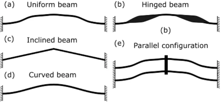
Pre-shaped bistable beams can be classified as uniform or hinged beam structures. The uniform beam has a simpler structure with uniform cross-section. However, the hinged beam has a variable cross-section along the beam length. The hinged shape is usually designed to promote some snap-through properties, such as symmetric bistability [50–53] or energy dissipation [54]. Uniform cross-section beams allow a more distributed compliance along their length. Hinged beams in contrast are constrained in their narrow parts where the deformation stress is more concentrated. This makes the use of uniform beams more efficient for miniaturiza-tion [45]. The study in this paper focuses on the case of uniform beams. Most reported uniform pre-shaped bistable beams have curved or inclined initial shapes. The curved shape is usually similar to the first mode shape of buckling of a straight beam. The inclined shape (V-shape) is easier to fabricate or assemble at macro-scale. Figure 1 shows the different pre-shaped beam types and configurations.
Curved beam Inclined beam
Uniform beam Hinged beam
Parallel configuration (a)
(b) (c)
(d)
(b)
(e)
Fig. 1. Examples of pre-shaped bistable beams.
Many analytical models have been reported for each kind of bistable beams and for the different modes of
ac-tuation. The modeling of bistable beams must account for the geometric nonlinearities associated with the simultane-ous lateral deflection and axial compression and the scenar-ios of bifurcation in the snap-through behavior.
For pre-shaped beams with a mid-length lateral force, Qiu et al. [44] developed a modal superposition solution for the initially curved shape based on energy variation calcu-lation and the classical beam theory. This work showed a bifurcation in the snap-through behavior of the curved beam where the second or third mode of buckling becomes acti-vated at a certain level of the axial stress. Using the same derivation, Hussein et al. [55] developed explicit analytical expressions of the snapping forces and internal stresses that account for all modes of buckling. A generalized model for arbitrarily initial shape and loading is developed in [56] and solved using two different iterative algorithms. A bilateral relationship between the first and second stable configura-tions of bistable pre-shaped beams was formulated in [57].
For initially inclined beams, Zhao et al. [58] developed an elliptic integral model based on large deformation the-ory where shear and axial deformation are negligible. This model is effective for thin and flexible beams where the ef-fects of axial elongation and shear are negligible [59]. In the same context, Holst et al. [60] considered the axial deflec-tion in their elliptic integral model. A curve decomposideflec-tion method is presented in [61] to simplify the large deforma-tion analysis. Chen et al. [62] used a beam constraint model from [63] and added a shear effect correction based on the Timoshennko theory to predict the snapping forces. The con-straint beam model was further extended in [64,65]. All cited modeling studies showed very good agreement with experi-ments and finite element method (FEM) simulations.
This work presents analytical study for the snap-through of an arbitrarily pre-shaped beam, subjected to a mid-length lateral point force. Explicit analytical expressions are de-rived describing the snap-through behavior, snapping forces and conditions for bifurcation, negative stiffness behavior, and bistability. The modeling is based on the classical beam theory, where the initial shape is expanded in Fourier series. The exact solution for the snap-through equation is derived considering all modes of buckling.
The snap-through governing expressions contain infinite sums depending on the modes of buckling and Fourier series coefficients. Some of these sums are already evaluated in [55], while the other sums are dependent on the initial shape. The infinite sums are evaluated for two initial shape cases, curved and inclined, and explicit analytical snap-through ex-pressions are obtained. The analytical modeling results are compared with FEM simulations for selected cases.
The rest of the paper is organized as follows. The snap-through solution for pre-shaped beams with arbitrarily initial shape is developed in Section 2. The snapping force solution for pre-shaped beams is then developed in Section 3. The calculations for a specific initial beam shape are clarified in Section 4 and the cases of pre-shaped curved and inclined beams are investigated. The snap-through behavior of both beam shapes is finally compared and discussed in Section 5.
2 Snap-through solution of a pre-shaped beam
The snap-through solution for a pre-shaped beam with an arbitrarily initial shape is developed in this section.
2.1 Problem definition and annotations
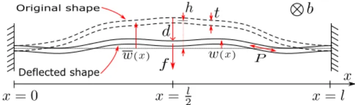
Figure 2 shows a schematic of a clamped-clamped pre-shaped beam deflected under a mid-length lateral point load
f. The beam has a spanl, in-plane thicknesst, initial middle heighth, and out-of-plane depthb.
Original shape
Deflected shape
Fig. 2. Schematic of a clamped-clamped pre-shaped beam.
The shape of the beam is described byw(x), which rep-resents the shape of the beam along thexaxis. w(x)refers to the original as-fabricated beam shape at zero deflection without any residual stress. The following assumptions are considered for the beam shape in this study:
◦ Clamped-clamped boundary conditions (l is constant,
w(x) =w(x),dwdx(x) =dwdx(x)forx=0,l).
◦ An initial middle heighth(w(l
2) =h).
◦ Uniform beam shape (bandtare constants).
◦ Small deformation hypothesis (t,h≪l).
◦ Symmetry of the initial shape with respect to the beam mid-length (w(l2−x) =w(2l +x)). This is usually the case for parallel configurations.
The deflectiondat the beam mid-length is defined as:
d=w(l
2)−w(
l
2) (1)
After deflection due to an applied point force f, the to-tal length of the beamsbecomes contracted and the internal axial forcePappears in the beam. In elastic structures, the axial force is calculated using Hooke’s law as follows:
P=EA
s−s
s
(2)
wheresis the initial beam length,Eis the Young’s modulus andAis the cross-section area.
Considering small deformation, the lengthsof the beam can be approximated as follows:
s=
l
0
s
1+
dw
dx
2
dx≈l+1
2
l
0
dw
dx
2
dx (3)
For convenience, we normalize the various variables as follows:
X=xl W(X) =w(hx) S= sl
h2 Q= h t
N=
q
Pl2
EI ∆=
d
h F=
f l3 EIh
(4)
whereIis the cross-section quadratic moment.
Considering uniform cross-section and material proper-ties, the static snap-through behavior of a pre-shaped beam subjected to an axial force and a lateral point load is governed by:
d4W dX4 −
d4W dX4 +N
2d2W
dX2 =4F
∑
j=1,5,9...
cosNjX (5)
The mathematical derivation of (5) is presented in Ap-pendix A. Nj is the jth critical buckling load. Mathemati-cally,Njis calculated to have a non-trivial solution after in-troducing the boundary conditions in the homogeneous prob-lem (similar to the probprob-lem of a straight beam). For clamped-clamped boundary conditions,Njis the jthpositive solution of the following periodic equation [44, 55]:
sinNj 2
tanNj 2 −
Nj 2
=0 (6)
Nj= (j+1)π j=1,3,5...
Nj=2.86π,4.92π,6.94π,8.95π... j=2,4,6...
(7)
2.2 Solution of the problem
In order to solve (5), W(X)is decomposed into three parts, the initial shapeW(X), a particular solutionWp, and a homogeneous solutionWh.
W(X) =W(X) +Wp(X) +Wh(X) (8) The consideration of the initial shapeW(X)accounts for the inhomogeneous boundary conditions. Thereby, introduc-ing (8) into (5), the problem can be decomposed into two separate problems with zero boundary conditions to find a particular and a homogeneous solution. The homogeneous problem is independent from the initial shape and external loads and is governed by the following equation:
d4Wh
dX4 +N 2d2Wh
dX2 =0 (9)
Equation (9) is the same equation governing a straight beam with an axial load. Its solution is an infinite superposi-tion of the modes of buckling as follows [44, 55]:
Wh(X) =
∞
∑
j=1
whereWj(X)is the jth mode shape of buckling and Aj is a constant that represents the contribution of the jth mode of buckling in the homogeneous solution. For clamped-clamped boundary conditions, Wj(X) is expressed as fol-lows:
(
Wj(X) =1−cosNjX j=1,3,5...
Wj(X) =1−cosNjX−2X+
2 sinNjX
Nj j=2,4,6...
(11)
Further, introducing (8) into (5), the particular problem is governed by the following equation:
d4Wp
dX4 +N 2
d2Wp
dX2 +
d2W dX2
=4F
∑
j=1,5,9...
cosNjX (12)
The initial shapeW(X) is usually symmetric between the two sides of the beam length. In parallel configurations, this symmetry serves for enhancing the bistability and to pro-duce a straight deflection of the shuttle at the mid-length of the beam. An arbitrarily initial shape, which is symmetric with respect to the beam mid-length, can be expanded using Fourier series over the beam length as follows:
W(X) =C0+
∑
j=1,3,5...
Cjcos(NjX) (13)
whereC0andCjare calculated as follows:
C0=
l
0
W dX Cj=2
l
0
Wcos(NjX)dX
(14)
Introducing the second derivative of (13) into (12), the particular problem equation becomes
d4Wp
dX4 +N 2d2Wp
dX2 =
∑
j=1,5,9...
(4F+CjN2jN2)cosNjX
+
∑
j=3,7,11...
CjN2jN2cosNjX
(15)
For each term cos(NjX) in (15), a particular solution
Wp j(X) satisfying zero boundary has the form Wp j(X) =
BjWj(X). Thereby, the particular solution has the following form:
Wp(X) =
∑
j=1,3,5...BjWj(X) (16)
whereBjis a constant that represents the contribution of the
jth mode of buckling in the particular solution. Bj are ob-tained by substituting (16) into (15):
Bj=
4F+CjN2jN2
N2
j(N2−N2j)
j=1,5,9...
Bj= CjN2
N2−N2
j
j=3,7,11...
Bj=0 j=2,4,6...
(17)
Thereby, combining (8), (10), and (16), the exact so-lution of the equilibrium equation in (5) has the following form:
W(X) =W(X) +
∞
∑
j=1
KjWj(X) (18)
whereKj=Aj+Bj.
The termsAjcan be calculated by introducing (10) into (9), which leads to the following:
∞
∑
j=1
N2j(N2−N2j)Ajcos(NjX) =0 (19)
According to (19), there is no contribution from the ho-mogeneous solution whenNis not at any of the critical buck-ling loadsNj:
Aj=0 forN6=Nj (20) The same conclusion can be extracted by minimizing the variation of the total energy of the system as in [44, 55]. Letub,uc,uf andutare the bending, compression, actuation and total energy and letU(·)=
u(·)l3
EIh2 is the normalization for each of them. The variation ofUb,Uc,Uf are calculated as follows:
∂Ub= 1 2∂
1
0
d2W dX2 −
d2W dX2
2
dX (21a)
∂Uc=−N2∂S (21b)
∂Uf =−F∂∆ (21c)
The variation of the total energy is the sum of bending, compression, and actuation energy variations:
∂Ut=
∑
j=1,5,9...(N2j−N2)Kj+ 4F N2j +CjN
2
!
N2j
2 ∂Kj
+
∑
j=3,7,11...
(N2j−N2)Kj+CjN2
N2j
2 ∂Kj
+
∑
j=2,4,6...
N2j−N2N
2
j 4 ∂K
2
j
.
Minimizing∂Ut, the expressions ofKj are obtained. In this case, it can be noticed thatKjare equivalent toBjin (17) forN6=Nj, which validates (20).
The energy variation calculation gives a further insight about the limitation ofN. WhenN starts to increase from zero after deflection between the two sides of buckling, N
cannot exceed N2 physically since ∂Ut is always positive. When N reaches N2 (if the geometry allows it), the
sec-ond mode of buckling becomes activated and changes the snap-through behavior of the pre-shaped beam. Note that
N reaches higher limits for higher values of the height-to-thickness ratioQ, as will be clarified latter.
The second mode can appear only in a single pre-shaped beam configuration, where a second stable position exists weakly only in some cases for high values ofQ. In paral-lel configurations, the non-symmetrical modes of buckling are constrained, which enhances the bistability and allows a guided straight range of motion of the shuttle at the beams mid-length [44, 55]. In this work, only the parallel configu-ration scenario is considered.
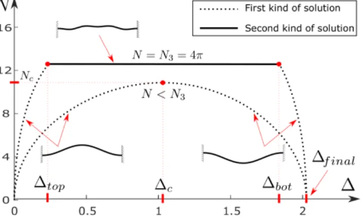
In parallel configurations, N is able to exceedN2 and
a bifurcation between two kinds of solution emerges at the third critical buckling loadN3. In the first kind, the
homoge-neous solution has no contribution (Aj=0 for j=1, ...,∞)
and it applies whenNis belowN3(N<N3). In the second
kind, the third mode in the homogeneous solution becomes activated (A36=0,Aj=0 for j6=3) and it applies whenN reachesN3(N=N3). As can be noticed from (17),Ncannot
reach N3 ifC36=0. Figure 3 demonstrates the variation of
N during deflection for two typical examples of pre-shaped curved beams. In the first example,Ncannot reachN3during
deflection whileN3is reachable in the second example. One
can note from Fig. 3 that the beam, in both cases, is more compressed in the middle zone of deflection, as evident from the high values ofN, while it is relaxed in the two sides of buckling. WhenN3is reached, the third mode of buckling
appears in the beam shape preventing any further compres-sion of the beam length. The occurrence of the two scenarios in Fig. 3 depends on the dimensional ratioQ; Ncan reach higher levels for higher values ofQ. Hence, the third mode of buckling get involved during deflection forQhigher than certain limit that will be determined in the next section.
In conclusion, the solution of the governing equation (5) has the form (18) whereKjare expressed as follows:
First kind
N<N3
Kj=
4F+CjN2jN2
N2
j(N2−N2j)
j=1,5,9...
Kj= CjN2
N2−N2
j
j=3,7,11...
Kj=0 j=2,4,6...
(23a)
Second kind
N=N3
Kj=
4F+CjN2jN32 N2
j(N32−N2j)
j=1,5,9...
Kj= CjN 2 3 N2
3−N2j
j=7,11,15...
Kj6=0,Cj=0 j=3
Kj=0 j=2,4,6...
(23b)
Fig. 3. Variation ofN during deflection for two examples of pre-shaped curved beams in parallel (constraint) configuration. The first example is whenN3is not reachable and the second is whenN3is
reachable during deflection.
The coefficientsKj are dependent onF,N, and∆. The relationship betweenF,N, and∆is determined from the de-flection equation (1) and Hooke’s law (2), as clarified in the next section.
3 Snapping force solution
The snapping force expressions are evaluated and ana-lyzed in this section. The snapping force is the mid-length lateral point force required to statically-balance the pre-shaped beam along the snap-through zone of deflection.
3.1 First kind of solution
Governing equations Introducing the solution from (18) and (23) into (1) and (2), the following equations are ob-tained governing the relationship betweenF,Nand∆:
F= 1
Λe(N)
(Λd(N)−∆) (24)
Λa(N)F2+Λb(N)F+Λc(N) +
N2
12Q2=0 (25)
whereΛa,Λb,Λc,ΛdandΛeare infinite sum functions that are dependent onNas follows:
Λa(N) =
∑
j=1,5,9...4
N2
j(N2−N2j)2
(26a)
Λb(N) =
∑
j=1,5,9..2CjN2j
(N2−N2
j)2
(26b)
Λc(N) =
∑
j=1,3,5...−C2jN2jN2
4
N2−2N2j
(N2−N2
j)2
(26c)
Λd(N) =
∑
j=1,5,9..−2CjN2
N2−N2
j
(26d)
Λe(N) =
∑
j=1,5,9...8
N2
j(N2−N2j)
(26e)
The infinite sums ΛaandΛe are independent from the initial shape. These sums were calculated in [55] for the case of a pre-shaped curved beam:
Λa(N) = 3 16N4 1−
tanN4 N
4
+tan
2N
4
3
!
(27a)
Λe(N) = 1
N3
N
4 −tan
N
4
(27b)
Equation (25) is a second order polynomial equation of
Fwhere the polynomial constants are dependent onN. Sim-ilarly, substituting (24) into (25), the resulting equation is a second order polynomial equation of ∆ where the
polyno-mial constants are dependent on N. This implies that for each value of N in the first kind of solution, there are two corresponding values ofFand∆; as clarified for the latter in Figure 3.
Maximum limit of axial compression The axial forceN
reaches a maximum levelNcin the middle zone of deflection as can be seen from Figure 3. The value ofNcincreases with increasing the dimensional ratio Q. The specific ratioQc, which allowsNto reach a maximum limitNcduring deflec-tion, is the minimum ofQthat allows obtaining real solutions forFatN=Ncin (25).Qcis then expressed as follows:
Qc=Nc
s
Λa(Nc)
3Λ2b(Nc)−12Λa(Nc)Λc(Nc)
(28)
CallingFcand∆cthe corresponding values forFand∆
for N=Ncrespectively; they can be determined from (24) and (25) as follows:
Fc=−
Λb(Nc) 2Λa(Nc)
(29a)
∆c=Λd(Nc) +
Λe(Nc)Λb(Nc) 2Λa(Nc)
(29b)
Note that the determination ofQcfrom (28) is limited to the rangeNc∈[0,N3]. Equation (28) helps to determine the
geometrical conditions to reach the different levels of axial compression, to have negative stiffness snap-through behav-ior, and to have a second kind of solution zone. In the sequel,
Q1,Q2andQ3refer to the values ofQcforNc=N1,N2and
N3, respectively.
Lateral stiffness The lateral stiffnessSof the beam in the snap-through zone is defined as (∂f/∂d), which is propor-tional to (∂F/∂∆). The stiffness expression can be deduced from (24) as follows:
S=EI
l3 ∂F
∂∆ =
EI l3
1
Λe
∂N
∂∆
∂Λd
∂N −F ∂Λe
∂N
−1
(30)
The lateral stiffnessS(which is proportional to the natu-ral frequency) decreases as the beam is compressed. This can be seen from the natural frequency as reported in [66]. Thus, in order to determine at which level the beam starts to show a negative stiffness behavior zone, we choose to calculate
S at the maximum axial stress point of deflection (N=Nc,
∆=∆c,F=Fc). At this point,(∂N/∂∆)is equal to zero by
definition, which gives the following expression of the stiff-ness:
SN=Nc=
EI l3
−1
Λe(Nc)
(31)
From the expression ofΛein (27b), we can deduce that the stiffnessSN=Nc is positive forNc∈[0,N1[, equal to zero
for Nc=N1and is negative for Nc∈]N1,N3]. This means
that a pre-shaped beam starts to show a negative stiffness behavior for aQvalue aroundQ1. Figure 4 shows the typical
snapping force curves for a pre-shaped curved beam in the three cases:Q<Q1,Q=Q1andQ1<Q<Q3.
Q<Q1
Q=Q1
Q1<Q<Q3
Fig. 4. Typical snapping force curves for a shallow pre-shaped curved beam withQ<Q1,Q=Q1andQ1<Q<Q3. Q1and
Q3refer to the values ofQcforNc=N1andN3, respectively.
As can be seen in Figure 4,Q1is the boundary between
different behaviors in terms of the lateral stiffness. For lower values ofQ, only positive stiffness behavior can be noticed.
ForQvalues close toQ1, the beam acts as a constant force
mechanism in the middle zone of deflection. However, this zero stiffness property is limited in terms of the range of displacement due to the small value ofQ1 in practice. For
higher values ofQ, the pre-shaped beam starts to show a neg-ative stiffness behavior around the middle zone of deflection. This negative stiffness zone is a necessary but insufficient condition to have bistability. The condition for bistability is that the snapping force reaches negative values during deflec-tion. In that case, the beam pushes itself to the second stable side instead of pushing back to the initial position. Note that the negative stiffness zone cannot be measured using a force-controlled experiment; a deflection control is required.
CallingFN1 and∆N1 the values ofFand∆, respectively, for Q=Q1andN=N1; we can notice from Figure 4 that
the snapping force curves for the different values ofQ for shallow beams (Q<Q3) pass in close vicinity of that point.
FN1 and∆N1 can be calculated from (29) by settingNc=N1.
Note thatFN1 is only dependent onC1as follows:
FN1=−4π4C1 (32)
Note also that the value of F for N=N1remains equal to
FN1, even forQ>Q1.
End of compression The limit of the snap-through deflec-tion zone where the soludeflec-tion developed in this paper remains applicable is the limit at whichN reaches zero after deflec-tion. After this limit, the beam becomes in tension (N<0), not in compression. Calling∆f inalandFf inalthe values of∆ andF at this limit, respectively; they can be deduced from (24) and (25) as follows:
∆f inal=−160 ∑
j=1,5,9..
Cj
N2
j
Ff inal=−30720 ∑
j=1,5,9..
Cj
N2j
(33)
Note that Ff inal is positive since it is proportional to
∆f inal, which is in the∆positive zone (Ff inal=192∆f inal).
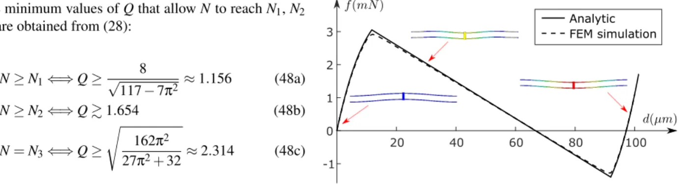
3.2 Second kind of solution
For the second kind of solution, N remains constant at
N3for a certain range of deflection. We callF3the snapping
force in the second kind of solution. The relation betweenF3
and∆in this range can be obtained from (24):
F3=64π2(Λd3−∆) (34)
whereΛb3,Λc3andΛd3are used instead ofΛb(N3),Λc(N3)
andΛd(N3)in the sequel, respectively.
Fig. 5. Typical snapping force curve for a pre-shaped curved beam withQ>Q3. Initially, the snapping force increases with increasing
the beam mid-point deflection, maintaining a shape defined by the 1st, 5th, 9th ... modes of buckling (1st mode is dominating), until reaching∆top. In between∆topand∆bot, the third mode of buckling
involves in addition in the shape of the beam, resulting in a constant negative stiffness behavior. After∆bot, the third mode of buckling
is no more involved and the snapping force increases with the de-flection. The negative stiffness in-between∆topand∆bot leads to
bistability (two zero-force positions with positive stiffness behavior at
∆=0 and at∆end).
The second kind of solution zone is reachable during deflection forQ≥Q3. The typical snapping force curve for
a pre-shaped curved beam in this case is shown in Figure 5. From (34) and Figure 5, one can notice that when-ever the initial shape of a pre-shaped beam allows reaching
N=N3, the lateral stiffness of the beam in the range of
de-flection of the second kind of solution(S3)is negative,
con-stant and is only dependent on the material strength and the beam dimensions (except for the initial heighth). However,
S3is independent from the specific initial shape of the beam,
as given below:
S3=−64π2EI
l3 (35)
The third mode constantK3in the second kind of
solu-tion can be calculated from the Hooke’s law. Mathematically,
K3is added in (25) in a way thatNremains equal toN3.
Re-call thatC3=0 is a condition forNto reachN3. Thereby,K3
is equivalent to:
K3=±
1 2π
s
− 3
4096π4F 2
3−Λb3F3−Λc3−
4π2
3Q2 (36)
Considering (34),K3can be expressed as a function of ∆:
K3=±
1 2π
v u u t
−3∆2+ (6Λd3+64π2Λb3)∆−4π
2
3Q2
−3Λ2d3−64π2Λb3Λd3−Λc3
The limits of the second kind of solution zone in terms of
∆andFcan be obtained from the expression ofK3. We label
(∆top,Ftop) at the first limit (closer to∆=0) and (∆bot,Fbot) at the second limit. ∆top,Ftop,∆bot andFbot are calculated at the limits where K3 in (36) and (37) has a real solution
(K3=0).
∆top=Λd3+
32π2Λb3
3 −
s 32
π2Λb3
3
2
−Λc3
3 −
4π2
9Q2
(38a)
Ftop=64π2
−32π2Λb3
3 +
s
32π2Λb3
3
2
−Λc3
3 −
4π2
9Q2
(38b)
∆bot=Λd3+
32π2Λb3
3 +
s
32π2Λb3
3
2
−Λc3
3 −
4π2
9Q2
(38c)
Fbot=64π2
−32π2Λb3
3 −
s
32π2Λb3
3
2
−Λc3
3 −
4π2
9Q2
(38d)
The snapping forces atFtopandFbot are practically the maximum positive and minimum negative reachable force levels between the stable sides in case of bistability, respec-tively.
3.3 Bistability of pre-shaped beams
A bistable pre-shaped beam have a negative snapping force in some range of the snap-through deflection. The neg-ative snapping force indicates that the beam is pushing itself to the other side of buckling. The bistability here refers to the ability of the beam to retain the static position without the application of external forces. In this case, the stable po-sition has a zero snapping force value (F=0).
An essential property for a stable position is the posi-tive stiffness, which means that the beam pushes back to the stable position after a slight deflection. In these conditions, the two stable positions are ∆=0 and ∆end, which satisfy zero snapping force and positive stiffness as shown in Figure 5. The second zero-force position∆mis an unstable position since the beam has a negative lateral stiffness around it. The values of∆mand∆endare calculated from (24) as follows:
∆m=Λd(Nm) (39a)
∆end=Λd(Nend) (39b)
The existence of the unstable position∆mindicates the existence of a negative force zone and thereby the bistability (Figure 5).∆mcan be located in both kinds of solution zone. However, the stable positions are always in the applicable
zone of the first kind of solution since the stiffness in the second kind of solution is negative (35). The second stable position ∆end has a positive value ofN (Figure 5, Nf inal = 0<Nend <Nbot=N3). Hence, it is sufficient to prove the
existence of at least one zero force solution F =0 of the first kind of solution governing expression (25) in the range
N∈(0,N3)to prove the bistability of a pre-shaped beam:
Bistability ⇐⇒ ∃N∈(0,N3),Λc(N) +
N2
12Q2=0 (40)
Note that the existence of the second kind of solution is not necessary for bistability. Note also that in a single beam configuration (second kind of solution applies forN=N2),
the bistability condition is that a solution of (40) exists for
N∈(0,N2).
The minimum ofQallowing a pre-shaped beam to have bistability is the minimum of Q that satisfies (40). Inde-pendently fromQ, we can extract from (40) thatΛc(N)for a bistable pre-shaped beam must have a negative value for some portion ofN∈(0,N3)in case of bistability.
The expression ofΛc(N)(26c) is an infinite sum of pos-itive components for N ∈(0,√2N1], while only the
com-ponent multiplied by C12 has a negative value in the range
N∈(√2N1,N3). Thereby, the condition of bistability in (40)
can be reformulated as follows:
Bistability ⇐⇒ ∃N∈(√2N1,N3),Λc(N)<0 (41)
In conclusion, the first mode of buckling in the initial shape of a pre-shaped beam (proportional to C1) must be
sufficiently dominant over the other modes of buckling to have bistability (since onlyC1makes a negative contribution
to satisfy (41)).This justifies the consideration of the curved shape as a common shape for a pre-shaped bistable beam. Further, in case (41) is satisfied, the minimum value ofQfor reaching bistability is the real minimum ofp−N2/12Λ
c(N) in the rangeN∈(√2N1,N3).
Furthermore, as the jth modes of buckling (j =
3,7,11, ...) are only involved inΛc(N)and add only positive contribution to Λc(N), which degrades the bistability (41), an initial shape without these modes of buckling will have a better bistability. In other words, if a pre-shaped beam is bistable and the Fourier series expansion for the initial shape includes componentsCjfor (j=3,7,11, ...), neglect-ing these components while keepneglect-ing the same components
Cjfor (j=1,5,9, ...) will result in a better bistability behav-ior. Considering the boundary conditions, onlyC0will be
changed after neglectingCj for (j=3,7,11, ...). C0in this
case is equivalent to 1/2. The simplest shape that satisfies this property is the inclined shape, which justifies its con-sideration as another common shape for a pre-shaped beam bistable mechanism.
4 Calculations for specific beam shapes
In the previous sections, derivations are developed for a general case with an arbitrarily initial shape. Calculations for specific initial shapes are presented in this section.
For a specific initial beam shapeW, the first step is to de-termine the corresponding Fourier series coefficientsCj(14). CoefficientsΛb,ΛcandΛd(26), are calculated for a specific initial shape. Then, the buckling mode constants Kj ((23) and (37)) are obtained. Introducing the different coefficients and constants, the snap-through solution (18) and snapping force expressions ((24), (25), (34)) are obtained. Afterwards, the different snapping points ((29), (32), (33), (38), (39)) and the conditions for reaching different levels of axial compres-sion (28) and for bistability (41) are determined. These steps are summarized in Table 1.
Table 1. Computational steps for the initial shape of beams.
Steps of calculation Equations 1 Fourier coefficientsC0andCj (14) 2 CoefficientsΛb,ΛcandΛd (14) in (26)
3 Buckling mode constantsKj
(14) in (23), (26) in (37) 4 Snap-through solution (23), (37) in (18)
5 Snapping force expressions (26), (27) in (24), (25), (34)
6 Snapping points
(14), (26), (27) in (29), (32), (33),
(38), (39)
7 Conditions for reaching levels of compression
(26), (27) in (28)
8 Bistability condition (26) in (41)
The analytical development in this paper considers all modes of buckling and Fourier series coefficients. The snapping force expressions ((24), (25)) governing the snap-through behavior contain infinite sums (26), where some of them are independent from the initial shape. The correspond-ing analytical expressions for these sums were calculated in [55] and are shown in (27). The other infinite sums need to be evaluated depending on the initial shape.
Two case studies are investigated in this section: curved and inclined initial beam shapes. Explicit analytical expres-sions corresponding to the infinite sums, depending on the initial shape, in both case studies are calculated consider-ing all Fourier series coefficients. However, for other initial shapes, where the calculation of the infinite sums is complex, finite number of Fourier series coefficients can be considered and convergence needs to be checked.
4.1 Pre-shaped curved beam
The curved shape (Figure 1.d) is similar to that of the first buckling mode; hence:
W =1
2W1 (42)
The Fourier series coefficientsC0andCjfor an initially curved beam are calculated from (14) as follows:
C0=12
Cj=−12 j=1
Cj=0 j=else
(43)
The snap-through solution for a pre-shaped curved beam has the form in (18) whereKj are calculated by introducing
Cjfrom (43) into (23):
First kind
N<N3
Kj=
4F−1 2N2jN2
N2
j(N2−N2j)
j=1
Kj=N2 4F
j(N2−N2j)
j=5,9,13...
Kj=0 j=3,7,11...
Kj=0 j=2,4,6...
(44a)
Second kind
N=N3
Kj=
4F−1 2N2jN2
N2j(N2−N2
j)
j=1
Kj=N2 4F
j(N2−N2j)
j=5,9,13...
Kj=0 j=7,11,15...
Kj6=0,Cj=0 j=3
Kj=0 j=2,4,6...
(44b)
The snapping force expressions for a pre-shaped curved beam for the first kind of solution are given in (24) and (25), whereΛb,Λc, andΛdare calculated as follows:
Λb(N) =
−4π2
(N2−4π2)2 (45a) Λc(N) =−
π2N2
4
N2−8π2
(N2−4π2)2 (45b) Λd(N) =
N2
N2−4π2 (45c)
Also, the snapping force expression in the second kind of solution is obtained from (34) as below:
F3=64π2
4
3−∆
(46)
The third mode constantK3in the second kind of
solu-tion is obtained from (37):
K3=±
1 2π
s
−3∆2+56
9 ∆+ 2π2
9 −
80 27−
4π2
The minimum values ofQthat allowNto reachN1,N2
andN3are obtained from (28):
∃N≥N1⇐⇒Q≥
8
√
117−7π2
≈1.156 (48a)
∃N≥N2⇐⇒Q&1.654 (48b)
∃N=N3⇐⇒Q≥
s
162π2
27π2+32≈2.314 (48c)
The condition on Qfor the bistability of a pre-shaped curved beam is obtained from (40):
Q≥√4
3≈2.309 (49)
The different snapping points coordinates are obtained from the modeling and are expressed as follows:
Ftop,Fbot=64π2 8
27± 2π
3
s
1 6+
16 81π2−
1
Q2
!
(50a)
∆top,∆bot= 28 27∓
2π
3
s
1 6+
16 81π2−
1
Q2 (50b)
∆m= 4
3 ∆end= 3 2+
s
1 4−
4
3Q2 (50c)
∆f inal= 20
π2 Ff inal=
3840
π2 (50d)
∆N1=
9 4−
π2
8 FN1=2π
4 (50e)
The axial force and snapping force curves for a shaped curved beam (Figures 3, 4, and 5) have been pre-sented in the previous section.
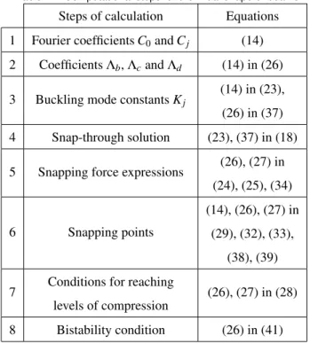
Figure 6 shows a comparison of the snapping force curves for a pair of pre-shaped curved beams in parallel con-figuration obtained analytically and with a nonlinear FEM model using the ANSYS software. The element ”PLANE82” was used in the FEM simulation with static analysis and con-sidering large deformation nonlinearity.
The mesh has been verified to be fine enough for con-vergence. The beam dimensions considered areb=25µm,
t =10µm, h =50µm, and l =2mm, while the material Young’s modulus is E =169GPa. The comparison shows excellent agreement between the two models.
It can be noticed that the solution and expressions de-rived in this section are similar to those obtained in [55]. This is due to the fact that the solution in [44, 55] is approximated as an infinite sum of the modes of buckling of a straight beam (same as for the homogeneous problem (11)) and the initial shape is similar to one of these modes of buckling.
20 40 60 80 100
-1 0 1 2 3
Analytic FEM simulation
Fig. 6. Snapping force comparison between the analytical and FEM models for a pair of pre-shaped curved beams in parallel configura-tion.
4.2 Pre-shaped inclined beam
The snapping behavior between the curved beam and the inclined beam is very similar qualitatively. However, the conditions, ranges, and levels are changed due to the differ-ent initial shape. The initial shape of a pre-shaped inclined beam (Figure 1.c) is described as follows:
W(X) =
2X X∈[0,12]
2−2X X∈[12,1] (51)
The Fourier series coefficientsC0andCjfor an initially inclined beam are calculated from (14) as follows:
C0=12
Cj=−N162
j
j=1,5,9...
Cj=0 j=else
(52)
The snap-through solution for a pre-shaped inclined beam has the form in (18) where Kj are calculated by in-troducingCjfrom (52) into (23):
First kind
N<N3
Kj= 4( F−4N2)
N2j(N2−N2
j)
j=1,5,9...
Kj=0 j=3,7,11...
Kj=0 j=2,4,6...
(53a)
Second kind
N=N3
Kj= 4( F−4N2)
N2
j(N2−N2j)
j=1,5,9...
Kj=0 j=7,11,15...
Kj6=0,Cj=0 j=3
Kj=0 j=2,4,6...
(53b)
The snapping force equations for a pre-shaped curved beam for the first kind of solution are given in (24) and (25) whereΛb,ΛcandΛdare infinite sums. However, considering
andΛe, which have their explicit expressions in (27), thus:
Λb(N) =−8N2Λa(N) +4Λe(N) (54a)
Λc(N) =16N4Λa(N)−16N2Λe(N) (54b)
Λd(N) =4N2Λe(N) (54c)
Subsequently, the snapping force relation in the second kind of solution is obtained from (34):
F3=64π2(1−∆) (55)
The third mode constantK3in the second kind of
solu-tion is obtained from (37):
K3=±
1 2π
s
−3∆2+4∆−4π 2
3Q2 (56)
The minimum values ofQ, which allowNto reachN1,
N2andN3, can be obtained from (28):
∃N≥N1⇐⇒Q≥ π2
4√3 ≈1.425 (57a)
∃N≥N2⇐⇒Q&2.080 (57b)
∃N=N3⇐⇒Q≥π≈3.142 (57c)
The condition on Qfor the bistability of a pre-shaped inclined beam is obtained from (40):
Q&3.196 (58)
The snapping force curves for a shallow pre-shaped in-clined beam (Q<Q3) are very similar to those presented in
Figure (4). However, the snapping force curve for (Q>Q3)
shows some differences, Figure 7.
The different snapping points coordinates are expressed as follows:
Ftop,Fbot=64π2
1 3±
2 3
s
1−π2
Q2
(59a)
∆top,∆bot= 2 3∓
2 3
s
1−π2
Q2 (59b)
∆m=1 ∆end:
N2
12Q2=1−
tanN4 N
4
−tan2N
4 (59c)
∆f inal= 5
3 Ff inal=320 (59d)
∆N1=
8
π2 FN1=16π
2 (59e)
Fig. 7. Snapping force curve for a shallow pre-shaped inclined beam.
The comparison between the analytical and FEM mod-eling results, for the same beam dimensions and material as in Figure 6, is shown in Figure 8 indicating excellent agree-ment.
10 20 30 40 50 60 70 80 -0.5
0 0.5
1 1.5
2
Analytic FEM simulation
Fig. 8. Snapping force comparison between the analytical and FEM models for a pair of pre-shaped inclined beams in parallel configura-tion.
In order to further demonstrate the accordance between the analytical modeling and FEM simulations, we choose to verify the accuracy of the bistability condition in (58). Figure 9 shows the snapping force curves obtained from FEM sim-ulations for a pair of inclined beams in parallel configuration with different values ofhand the same other dimensions and material as in Figure 8. The values ofhare chosen asQ=3, 3.2 and 3.5.
As explained in Section 3.3, the beam with negative snapping force pushes itself to the other side of buckling which leads to bistability. One can notice from Figure 9 that the snapping force curve starts to reach the negative force zone forQclose to 3.2 and higher, in agreement with (58).
5 Comparison and discussion
The snap-through behavior and the snapping force curves show some similarities and differences between pre-shaped curved and inclined beams in terms of forces, po-sitions and Q limits. These difference and similarities are
Fig. 9. Snapping force curves for a pair of pre-shaped inclined beams in parallel configuration with different values ofQ.
investigated and discussed in this section.
5.1 Conditions onQ
Table 2 shows theQratios, for both curved and inclined beams, after whichNcan reachN1,N2andN3and the
mini-mumQratios for bistability in both single and parallel con-figuration. One can note that the axial forceNreaches higher levels and the bistability occurs at lower values ofQfor the pre-shaped curved beam. This is more desirable for the de-sign of bistable mechanisms.
Table 2. MinimumQratios for reaching N1, N2 andN3and for
bistability.
Curved beam Inclined beam
N1 √ 8
117−7π2 ≈1.156
π2
4√3≈1.425
N2 ≈1.654 ≈2.080
N3
q
162π2
27π2+32≈2.314 π≈3.142
Bistability single ≈5.646 Never
Bistability parallel √4
3≈2.309 ≈3.196
5.2 Shallow beams
For shallow beams with low values ofQ, a second stable position does not exist but an interesting behavior is noticed. Increasing the value of Q, the snapping force curves show a transition between only positive stiffness behavior during deflection to the existence of zero stiffness and negative stiff-ness zones (Figure 4). This transition in the behavior occurs at the limit ofQ=Q1whereNstarts to reachN1. Figure 10
shows a comparison of the snapping force curves during de-flection forQ=Q1for both pre-shaped curved and inclined
beams.
0.5 1 1.5 2
0 100 200
300 Inclined beam
Curved beam
Fig. 10. Comparison of snapping force curves for pre-shaped curved and inclined beams forQ=Q1. Q1candQ1icorrespond
toQ1values for the curved and inclined beams, respectively. Q(.) refers toQ1corQ1idepending on the corresponding curve.
As Q1 is different between the curved and inclined
beams, the curve of the inclined beam in Figure 10 is mul-tiplied by a correction factor in force and displacement to enable a suitable frame for comparison. Considering the cor-rection factor and the normalized parameters, the compari-son in Figure 10 is between two beam types, which have the same material properties and dimensions, except forhwhich is different due to the difference inQ1. Figure 10 shows an
interesting accordance in the snapping force curves between both cases.
5.3 Bistable beams
The third mode of buckling get involved during deflec-tion when the critical buckling load is reached and the lateral stiffness becomes negative and constant. Practically, both beam initial shapes under comparison show bistability with the involvement of the third mode of buckling.
Figure 11 shows a comparison in the snapping force curves of the curved and inclined beams when the third mode of buckling is reachable. Considering normalized parameters in the comparison means that both beams have the same ma-terial and dimensions. As seen, the inclined beam has lower range of force and displacement.
0.5 1
1.5
2
-200 0 200 400
600 Inclined beam
Curved beam
Fig. 11. Comparison of snapping force curves for bistable pre-shaped beams.
At the start of deflection, the stiffness of the inclined beam is higher. However, the third mode gets involved ear-lier, which limits the force level that can be reached.
Further, both beams show exactly the same constant and negative stiffness during the involvement of the third mode of buckling. This is the general case for the stiffness of pre-shaped beams S3in the second kind of solution (35). Note
that the stiffnessS3is independent of the initial heighth.
The normalized force and range of displacement for both pre-shaped beams is highly dependent onQ. Figures 12, 13 and 14 show the variation with respect toQof Ftop, as a measure of the maximum snapping force level,∆end, as the distance between the two stable positions, andFbot over
Ftopas a measure of the symmetry between the two stable sides. The snap-through behavior is more symmetric when
|Fbot/Ftop|is closer to 1.
2 4 6 8 10
0 200 400 600
Inclined beam Curved beam
Fig. 12. Variation ofFtopwithQfor curved and inclined beams.
0.5 1 1.5 2
2 4 6 8 10
0
Inclined beam Curved beam
Fig. 13. Variation of∆endwithQfor curved and inclined beams.
6 Conclusions
In this paper, we derived the snap-through solution and the analytical expressions governing the snapping force of an arbitrarily pre-shaped elastic beam deflected under a mid-length lateral point force. The exact solution was calculated based on the classical beam theory and considering all modes of buckling. The snap-through behavior was analyzed based on the analytical expressions. The different snapping points and conditions for negative stiffness, bifurcation of solutions and bistability were clarified. The elements presented in this study constitute design tools for pre-shaped beams.
0.1 0.2 0.3 0.4
2 4 6 8 10
0
Inclined beam Curved beam
Fig. 14. Variation of|Fbot
Ftop|withQfor curved and inclined beams.
The calculation procedure for a specific initial shape was demonstrated. The derivations for two initial shapes, curved and inclined, were then investigated. The analyti-cal expressions in both cases were elaborated in explicit for-mulations considering all modes of buckling.The analytical modeling showed very good agreement with the FEM sim-ulations. Several similarities and differences were noticed in their snap-through behavior. The curved beam shows a wider margin of stability in the second stable side with more symmetric snap-through behavior, while the inclined beam requires larger height-to-thickness ratio to have bistability.
Acknowledgment
This research has been supported by KAUST research fund.
A Equilibrium equation
The static equilibrium equation (5) for a pre-shaped beam with a mid-length lateral point force is developed here-inafter based on the classic theory of elastic beams.
Figure 15.a shows a pre-shaped beam with an arbitrarily initial shape before and after deflection due to a mid-length lateral force. Even if the initial shape (w(x)) is symmetric with respect to the middle of the beam length, the beam shape (w(x)) is not necessarily symmetric after deflection.
Figure 15.b shows the forces and moments applied on the beam. The force equilibrium in both directions and the moment equilibrium at A and B give the following:
PA=PB=P (60a)
FA=FB=
f
2 (60b)
Considering small deformation hypothesis, the bending momentMxat the cross section of the beam is expressed as follows:
Mx=EI
d2w
dx2 −
d2w
dx2
(61)
From the static equilibrium, the expression ofMxis dif-ferent before and after beam mid-span where f is applied.
Fig. 15. A pre-shaped beam in deflection (a), forces and moments on the boundaries (b), on a section in the zonex∈[0,l2](c) and on a section in the zonex∈[2l,l](d).
Considering a section in the zonex∈[0,2l](Figure 15.c), the static equilibrium gives the following expression ofMx:
Mx=MA−Pw+
f
2x (62)
For a section in the zonex∈[l
2,l](Figure 15.d),Mxis expressed as follows:
Mx=MA−Pw+
f
2(l−x) (63)
Combining (61), (62) and (63), the equilibrium equation becomes as follows:
EI
d2w dx2 −
d2w dx2
+pw=MA+
f
2
x x∈[0,2l]
l−x x∈[2l,l] (64)
Considering a uniform cross-section and material prop-erties, deriving one time with respect toxto get rid ofMA, and considering the normalized parameters from (4), the equilibrium equation (64) becomes:
d3W dX3 −
d3W dX3 +N
2dW
dX = F
2Ψ(X) (65)
whereψ(x)is a discontinuous step function:
Ψ(X) =
1 X∈[0,12]
−1X∈[12,1] (66)
As the problem has four boundary conditions, the equi-librium equation is represented in the fourth order form:
d4W dX4 −
d4W dX4 +N
2d2W
dX2 =
F
2
dΨ
dX(X) (67)
The discontinuous step functionψ(X)can be expanded in Fourier series over the beam length as follows:
Ψ(X) = ∑
j=1,5,9... 8
NjsinNjX X∈[0,1] (68)
whereNj= (j+1)πis the critical buckling load for
symmet-ric modes of buckling as shown in (7).
The Fourier series expansion helps to determine the derivatives ofψ(X)and to quantify the effect of the lateral
force f on each mode of buckling. From the derivative of (68), we can notice that:
dΨ
dX(X) =δ(X) +δ(X−1)−2δ(X−
1
2) (69)
whereδ(X)is an impulse function over[0,1]domainδ(X) =
1 X=0 0 X∈(0,1].
Introducing the derivative of (68) into (67), equation (5) is obtained.
d4W dX4 −
d4W dX4+N
2d2W
dX2 =4F
∑
j=1,5,9...
cosNjX (70)
References
[1] Zirbel, S. A., Tolman, K. A., Trease, B. P., and Howell, L. L., 2016. “Bistable Mechanisms for Space Applica-tions”. PLoS One,11(12), dec, p. e0168218.
[2] Ben Salem, M., Aiche, G., Rubbert, L., Renaud, P., and Haddab, Y., 2018. “Design of a Microbiota Sam-pling Capsule using 3D-Printed Bistable Mechanism”. In Proc. Annu. Int. Conf. IEEE Eng. Med. Biol. Soc. EMBS, Vol. 2018-July, pp. 4868–4871.
[3] Ando, B., Baglio, S., L’Episcopo, G., and Trigona, C., 2012. “Investigation on Mechanically Bistable MEMS Devices for Energy Harvesting From Vibrations”. J. Microelectromechanical Syst.,21(4), aug, pp. 779–790. [4] Vysotskyi, B., Aubry, D., Gaucher, P., Le Roux, X., Parrain, F., and Lefeuvre, E., 2018. “Nonlinear electro-static energy harvester using compensational springs in gravity field”. J. Micromechanics Microengineering,
28(7), jul, p. 074004.
[5] Hajjaj, A. Z., Jaber, N., Ilyas, S., Alfosail, F. K., and Younis, M. I., 2020. “Linear and nonlinear dy-namics of micro and nano-resonators: Review of re-cent advances”. Int. J. Non. Linear. Mech.,119, mar, p. 103328.
[6] Wang, N., Cui, C., Chen, B., Guo, H., and Zhang, X., 2019. “Design of Translational and Rotational Bistable Actuators Based on Dielectric Elastomer”. J. Mech. Robot.,11(4), aug.
[7] Hansen, B. J., Carron, C. J., Jensen, B. D., Hawkins, A. R., and Schultz, S. M., 2007. “Plastic latching ac-celerometer based on bistable compliant mechanisms”.
Smart Mater. Struct.,16(5), oct, pp. 1967–1972. [8] Frangi, A., De Masi, B., Confalonieri, F., and Zerbini,
S., 2015. “Threshold Shock Sensor Based on a Bistable Mechanism: Design, Modeling, and Measurements”.
J. Microelectromechanical Syst.,24(6), dec, pp. 2019– 2026.
[9] Jaber, N., Ilyas, S., Shekhah, O., Eddaoudi, M., and Younis, M. I., 2018. “Resonant Gas Sensor and Switch Operating in Air with Metal-Organic Frame-works Coating”. J. Microelectromechanical Syst.,
27(2), apr, pp. 156–163.
[10] Hajjaj, A., Chappanda, K., Batra, N., Hafiz, M., Costa, P., and Younis, M., 2019. “Miniature pressure sensor based on suspended MWCNT”. Sensors Actuators A Phys.,292, jun, pp. 11–16.
[11] Kessler, Y., Ilic, B. R., Krylov, S., and Liberzon, A., 2018. “Flow Sensor Based on the Snap-Through De-tection of a Curved Micromechanical Beam”.J. Micro-electromechanical Syst.,27(6), dec, pp. 945–947. [12] Truong, Q.-D., Tran, N.-D.-K., and Wang, D.-A., 2017.
“Design and characterization of a mouse trap based on a bistable mechanism”.Sensors Actuators A Phys.,267, nov, pp. 360–375.
[13] Du, H., Chau, F. S., and Zhou, G., 2018. “Harmonically-Driven Snapping of a Micromachined Bistable Mechanism with Ultra-Small Actuation Stroke”. J. Microelectromechanical Syst.,27(1), feb, pp. 34–39.
[14] Qiu, J., Lang, J. H., Slocum, A. H., and Weber, A. C., 2005. “A bulk-micromachined bistable relay with u-shaped thermal actuators”. Microelectromechanical Systems, Journal of,14(5), pp. 1099–1109.
[15] Gomm, T., Howell, L. L., and Selfridge, R. H., 2002. “In-plane linear displacement bistable microre-lay”.J. Micromechanics Microengineering,12(3), may, pp. 257–264.
[16] Charlot, B., Sun, W., Yamashita, K., Fujita, H., and Toshiyoshi, H., 2008. “Bistable nanowire for microme-chanical memory”.Journal of Micromechanics and Mi-croengineering,18(4), feb, p. 045005.
[17] Hafiz, M. A. A., Kosuru, L., and Younis, M. I., 2016. “Microelectromechanical reprogrammable logic device”.Nature communications,7, p. 11137.
[18] Alfattani, R., and Lusk, C., 2018. “A Lamina-Emergent Frustum Using a Bistable Collapsible Com-pliant Mechanism”. J Mech Design, 140(12), sep, p. 125001.
[19] Chen, G., and Zhang, S., 2011. “Fully-compliant statically-balanced mechanisms without prestressing assembly: concepts and case studies”.Mech. Sci.,2(2), aug, pp. 169–174.
[20] Rafsanjani, A., Bertoldi, K., and Studart, A. R., 2019. “Programming soft robots with flexible mechanical metamaterials”.Science Robotics,4(29), p. eaav7874. [21] Xu, Q., 2017. “Design of a large-stroke bistable
mech-anism for the application in constant-force microposi-tioning stage”.J. Mech. Robot.,9(1), dec, p. 011006. [22] Wang, P., and Xu, Q., 2018. “Design and modeling of
constant-force mechanisms: A survey”. Mech. Mach. Theory,119, pp. 1–21.
[23] S¨onmez, U., and Tutum, C. C., 2008. “A Compli-ant Bistable Mechanism Design Incorporating Elas-tica Buckling Beam Theory and Pseudo-Rigid-Body Model”. J Mech Design,130(4), apr, p. 042304. [24] Wilcox, D., and Howell, L., 2005. “Fully compliant
tensural bistable micromechanisms (FTBM)”. J. Mi-croelectromechanical Syst.,14(6), dec, pp. 1223–1235. [25] Masters, N., and Howell, L., 2003. “A self-retracting fully compliant bistable micromechanism”. J. Micro-electromechanical Syst.,12(3), jun, pp. 273–280. [26] Hwang, I.-H., Shim, Y.-S., and Lee, J.-H., 2003.
“Mod-eling and experimental characterization of the chevron-type bi-stable microactuator”. J. Micromechanics Mi-croengineering,13(6), nov, pp. 948–954.
[27] Chen, G., Han, Q., and Jin, K., 2020. “A Fully Compli-ant Tristable Mechanism Employing Both Tensural and Compresural Segments”.J. Mech. Robot.,12(1), feb. [28] Hussein, H., Bouhadda, I., Mohand-Ousaid, A.,
Bour-bon, G., Le Moal, P., Haddab, Y., and Lutz, P., 2018. “Design and fabrication of novel discrete actuators for microrobotic tasks”. Sensors and Actuators A: Physi-cal,271, pp. 373–382.
[29] Zanaty, M., Vardi, I., and Henein, S., 2018. “Pro-grammable Multistable Mechanisms: Synthesis and Modeling”. J Mech Design,140(4), feb, p. 042301. [30] Che, K., Yuan, C., Wu, J., Jerry Qi, H., and Meaud,
J., 2016. “Three-Dimensional-Printed Multistable Me-chanical Metamaterials With a Deterministic Deforma-tion Sequence”.J Appl Mech,84(1), oct, p. 011004. [31] Chen, G., Gou, Y., and Zhang, A., 2011. “Synthesis
of compliant multistable mechanisms through use of a single bistable mechanism”. J Mech Design, 133(8), p. 081007.
[32] Chalvet, V., Haddab, Y., and Lutz, P., 2013. “A mi-crofabricated planar digital microrobot for precise posi-tioning based on bistable modules”.IEEE Transactions on Robotics,29(3), pp. 641–649.
[33] Vangbo, M., 1998. “An analytical analysis of a com-pressed bistable buckled beam”. Sensors Actuators A Phys.,69(3), sep, pp. 212–216.
[34] Alkharabsheh, S. A., and Younis, M. I., 2013. “Stat-ics and dynam“Stat-ics of mems arches under axial forces”.
Journal of Vibration and Acoustics,135(2), p. 021007. [35] Camescasse, B., Fernandes, A., and Pouget, J., 2013. “Bistable buckled beam: Elastica modeling and anal-ysis of static actuation”. Int. J. Solids Struct., 50(19), sep, pp. 2881–2893.
[36] Gerson, Y., Krylov, S., and Ilic, B., 2010. “Electrother-mal bistability tuning in a large displacement micro
ac-tuator”. Journal of Micromechanics and Microengi-neering,20(11), p. 112001.
[37] Michael, A., Kwok, C. Y., Yu, K., and Mackenzie, M. R., 2008. “A novel bistable two-way actuated out-of-plane electrothermal microbridge”. Journal of Mi-croelectromechanical Systems,17(1), pp. 58–69. [38] Chiao, M., and Lin, L., 2000. “Self-buckling of
micro-machined beams under resistive heating”. Journal of Microelectromechanical systems,9(1), pp. 146–151. [39] Lorenzoni, M., Llobet, J., and Perez-Murano, F., 2018.
“Study of buckling behavior at the nanoscale through capillary adhesion force”. Appl. Phys. Lett.,112(19), may, p. 193102.
[40] Pane, I. Z., and Asano, T., 2008. “Investigation on Bistability and Fabrication of Bistable Prestressed Curved Beam”. Jpn. J. Appl. Phys., 47(6), jun, pp. 5291–5296.
[41] Fang, W., and Wickert, J. A., 1994. “Post buckling of micromachined beams”. J. Micromechanics Micro-engineering,4(3), sep, pp. 116–122.
[42] Tajaddodianfar, F., Pishkenari, H. N., Yazdi, M. R. H., and Miandoab, E. M., 2015. “Size-dependent bistabil-ity of an electrostatically actuated arch NEMS based on strain gradient theory”.J. Phys. D. Appl. Phys.,48(24), jun, p. 245503.
[43] Krylov, S., Ilic, B. R., and Lulinsky, S., 2011. “Bistabil-ity of curved microbeams actuated by fringing electro-static fields”.Nonlinear Dyn.,66(3), nov, pp. 403–426. [44] Qiu, J., Lang, J., and Slocum, A., 2004. “A Curved-Beam Bistable Mechanism”. J. Microelectromechani-cal Syst.,13(2), apr, pp. 137–146.
[45] Hussein, H., Le Moal, P., Younes, R., Bourbon, G., Haddab, Y., and Lutz, P., 2019. “On the design of a preshaped curved beam bistable mechanism”. Mech. Mach. Theory,131, pp. 204–217.
[46] Park, S., and Hah, D., 2008. “Pre-shaped buckled-beam actuators: Theory and experiments”.Sensors Actuators A Phys.,148(1), nov, pp. 186–192.
[47] Aimmanee, S., and Tichakorn, K., 2018. “Piezoelectri-cally induced snap-through buckling in a buckled beam bonded with a segmented actuator”. J. Intell. Mater. Syst. Struct.,29(9), may, pp. 1862–1874.
[48] Camescasse, B., Fernandes, A., and Pouget, J., 2014. “Bistable buckled beam and force actuation: Experi-mental validations”. Int. J. Solids Struct., 51(9), may, pp. 1750–1757.
[49] Cazottes, P., Fernandes, A., Pouget, J., and Hafez, M., 2009. “Bistable buckled beam: modeling of actuating force and experimental validations”. J Mech Design,
131(10), p. 101001.
[50] Chen, Q., Zhang, X., Zhang, H., Zhu, B., and Chen, B., 2019. “Topology optimization of bistable mechanisms with maximized differences between switching forces in forward and backward direction”.Mech. Mach. The-ory,139, sep, pp. 131–143.
[51] Gao, R., Li, M., Wang, Q., Zhao, J., and Liu, S., 2018. “A novel design method of bistable structures with re-quired snap-through properties”. Sensors Actuators A
Phys.,272, apr, pp. 295–300.
[52] Huang, Y., Zhao, J., and Liu, S., 2016. “Design op-timization of segment-reinforced bistable mechanisms exhibiting adjustable snapping behavior”. Sensors and Actuators A: Physical,252, pp. 7–15.
[53] Tran, N. D. K., and Wang, D.-A., 2017. “Design of a crab-like bistable mechanism for nearly equal switch-ing forces in forward and backward directions”.Mech. Mach. Theory,115, pp. 114–129.
[54] Chen, Q., Zhang, X., and Zhu, B., 2018. “Design of buckling-induced mechanical metamaterials for energy absorption using topology optimization”. Struct. Mul-tidiscip. Optim.,58(4), oct, pp. 1395–1410.
[55] Hussein, H., Le Moal, P., Bourbon, G., Haddab, Y., and Lutz, P., 2015. “Modeling and Stress Analysis of a Pre-Shaped Curved Beam: Influence of High Modes of Buckling”. Int. J. Appl. Mech.,07(04), p. 1550055. [56] Williams, M. D., van Keulen, F., and Sheplak, M.,
2012. “Modeling of Initially Curved Beam Structures for Design of Multistable MEMS”.J Appl Mech,79(1), jan, p. 011006.
[57] Palathingal, S., and Ananthasuresh, G. K., 2019. “Anal-ysis and Design of Fixed–Fixed Bistable Arch-Profiles Using a Bilateral Relationship”.J. Mech. Robot.,11(3), jun.
[58] Zhao, J., Jia, J., He, X., and Wang, H., 2008. “Post-buckling and Snap-Through Behavior of Inclined Slen-der Beams”.J Appl Mech,75(4), jul, p. 041020. [59] Zhang, A., and Chen, G., 2013. “A Comprehensive
Elliptic Integral Solution to the Large Deflection Prob-lems of Thin Beams in Compliant Mechanisms”. J Mech Robot,5(2), mar, p. 021006.
[60] Holst, G. L., Teichert, G. H., and Jensen, B. D., 2011. “Modeling and Experiments of Buckling Modes and Deflection of Fixed-Guided Beams in Compliant Mechanisms”.J Mech Design,133(5), may, p. 051002. [61] Kim, C., 2011. “Curve Decomposition Analysis for Fixed-Guided Beams With Application to Statically Balanced Compliant Mechanisms”. In Vol. 6 35th Mech. Robot. Conf. Parts A B, ASME, pp. 149–158. [62] Chen, G., and Ma, F., 2014. “Kinetostatic Modeling
of Fully Compliant Bistable Mechanisms Using Tim-oshenko Beam Constraint Model”. J Mech Design,
137(2), feb, p. 022301.
[63] Awtar, S., Slocum, A. H., and Sevincer, E., 2007. “Characteristics of Beam-Based Flexure Modules”. J Mech Design,129(6), jun, p. 625.
[64] Ma, F., and Chen, G., 2017. “Bi-BCM: A Closed-Form Solution for Fixed-Guided Beams in Compliant Mech-anisms”.J. Mech. Robot.,9(1), feb.
[65] Chen, G., Ma, F., Hao, G., and Zhu, W., 2019. “Mod-eling Large Deflections of Initially Curved Beams in Compliant Mechanisms Using Chained Beam Con-straint Model”. J. Mech. Robot.,11(1), feb.
[66] Nayfeh, A. H., and Emam, S. A., 2008. “Exact solution and stability of postbuckling configurations of beams”.