ORIGINAL RESEARCH
Autoencoder for wind power prediction
Sumaira Tasnim
1, Ashfaqur Rahman
2*, Amanullah Maung Than Oo
1and Md. Enamul Haque
1Abstract
Successful integration of renewable energy sources like wind power into smart grids largely depends on accurate
prediction of power from these intermittent sources. Production of wind power cannot be controlled as the wind
speed can vary based on weather conditions. Accurate prediction of wind power can assist smart grid that
intelli-gently decides on the usage of alternative power sources based on demand forecast. Time series wind speed data are
normally used for wind power prediction. In this paper, we have investigated the usage of a set of secondary features
obtained using deep learning for wind power prediction. Deep learning is a special form on neural network that is
capable of capturing the structural properties of time series data in terms of a set of numeric features. More precisely,
we have designed a two-stage autoencoder (a particular type of deep learning) and incorporated the structural
fea-tures into a prediction framework. Using the structural feafea-tures, we have achieved as high as 12.63% better prediction
accuracy than traditionally used statistical features.
© The Author(s) 2017. This article is distributed under the terms of the Creative Commons Attribution 4.0 International License (http://creativecommons.org/licenses/by/4.0/), which permits unrestricted use, distribution, and reproduction in any medium, provided you give appropriate credit to the original author(s) and the source, provide a link to the Creative Commons license, and indicate if changes were made.
Introduction
Renewable energy sources like wind are becoming
inte-gral part of modern power systems. As reported in
IRENA (2017), renewable energy accounts for around
22% of global power generation. This share is expected
to double in the next 15 years. This is due to the rapid
growth of variable renewable energy from sources like
wind and solar photovoltaic (IRENA 2017). Renewable
energy offers several advantages such as easy availability,
applicability, and environmental friendly. The application
of smart grid in renewable energy makes it even more
promising. Smart grid engineering is the key for a
ben-eficial use of widespread energy resources. This fusion of
smart grid and renewable energy enables the efficient use
of such sources.
Alongside offering the opportunities, integration of
renewable energy like wind power into smart grids is not
without challenges. The key issue is being the
intermit-tent nature of wind power. The wind speed varies and so
is the power produced from wind-driven power station.
Also the produced energy needs to be consumed
imme-diately unless that is stored at additional cost. It is thus
highly beneficial to know in advance the amount of wind
power that can be expected. It is also important from
demand management point of view. Fossil fuel supplies
for power generation can be adjusted based on expected
demand. That is, however, not possible for wind energy
sources for the reasons explained above.
Prediction/fore-casting of wind power is thus a necessity for integrating
wind energy into smart grids.
Wind power prediction methods are developed to deal
with this problem and aim to predict generated power
based on historical weather/wind data by utilising data
mining methods (Wang et al. 2011,
2016; Colak et al.
2012; Soman et al. 2010; Zhao et al. 2016; Jiang et al.
2017). In general, historical wind data obtained from
weather stations are used by data mining algorithms to
make the predictions. Wind data over time is time series
data. Traditional data mining approaches model
pre-dicted wind power as a function of raw wind data over
a period of time. A wind power prediction method was
previously attempted in Tasnim et al. (2014) by
mod-elling predictions as a function of statistical features
extracted from raw time series data. Promising results
were reported when the ensemble feature-based
predic-tion framework was adopted.
The trend of investigating new feature
representa-tions for day-ahead wind power prediction is continued
Open Access
*Correspondence: [email protected]
2 Data61, CSIRO, 15 College Rd, Sandy Bay, TAS 7005, Australia
in our research presented in this paper. In this particular
research work, feature representations are learnt using a
particular kind of deep learning algorithm called stacked
autoencoders (Ng et al. 2016; Bengio et al. 2007; Shin
et al.
2014). Autoencoders generate a compressed
low-dimensional structural representation of the time series
(Bengio et al. 2007). A stacked autoencoder obtains
struc-tural representations (i.e. features) at multiple stages by
repeated application of autoencoders on the compressed
feature space. Supervised learning algorithms are trained
on the compressed feature space. State-of-the-art
learn-ing performance was achieved by stacked autoencoders
on images (Vincent et al. 2010; Gehrig et al. 2013), speech
(Gehrig et al. 2013), agricultural applications
(Rah-man et al. 2016), and other structured time series (Shin
et al.
2011) signals. This paper investigates whether the
stacked autoencoder provides an effective representation
for wind power prediction. In previous studies (Tasnim
et al.
2014), an ensemble framework was considered for
wind power prediction. For the sake of completeness, we
also embedded the autoencoder features in cluster-based
ensemble framework in Rahman and Verma (2011) and
Rahman et al. (2010) and investigated its effectiveness as
part of the framework too.
To the best of our knowledge, incorporation of
autoen-coder features in day-ahead wind power prediction
framework is a novel idea and we consider this as the
key contribution in this research. We have investigated
the following research questions in this paper: (1)
inves-tigating the effectiveness of autoencoder features for
wind power prediction, (2) comparing the performance
of autoencoder features to statistical features for wind
power prediction, and (3) how much improvement do
we achieve by embedding the autoencoder features in
ensemble framework. Experimental results reveal that
we achieved as high as 12.63% improvement by using
autoencoder features over statistical features.
Proposed prediction framework
The prediction framework has normally two
compo-nents: training and prediction module. During training,
historical time series data are split into small time
win-dows and prediction targets are set for each window.
Fea-ture vectors are computed from each time window. This
produces a 2D (
two-dimensional
) matrix where each row
represents a feature vector. The targets are presented in
a column vector where
i
th entry is the target for the
i
th
row in the 2D matrix. A regression algorithm is trained
on these matrices to produce a model that can reproduce
the targets (with minimum error) given the input vectors
from the 2D matrix. During prediction, data available
up-to-date are windowed and presented to the
regres-sion model to produce the predictions in the future. In
this paper, we have investigated autoencoder features and
also their effectiveness as part of cluster-based ensemble
learning algorithms. We present both in this section. For
the sake of completeness, we present the statistical
fea-tures as well.
Statistical features
We need to specify the structure of the input vector and
target for training the regression models. We have used
wind power as the target that needs to be predicted. Let
ws
=
(
ws
0,
ws
1, …,
ws
n−1)
be the vector representing the
wind speed over
n
consecutive days. A set of
m
statisti-cal features
s
=
s
1,
s2
, …,
s
mare computed from the wind
speed vector
ws
and the vector
s
as the input vector for
the regression algorithm. The features were computed
from the time and frequency domain representations of
the wind speed vector
ws
.
Discrete Fourier
transforma-tion
(DFT) was applied on
ws
to obtain the frequency
domain representation of the time series data. Let
ws
tbe
the
t
th element of the time series. The
j
th element of the
frequency domain representation is obtained as:
where
n
is the length of the vector. Here
ws
represents the
wind speed at various points in time and
f
represents the
signal strength at various frequencies. We have used the
DC (
direct current
) component of the DFT (
f
0:
compo-nent corresponding to 0 frequency) as a feature. A set of
statistical features are then computed from the
remain-ing high-frequency (> 0) spectrum of
f
. The following
statistical features are computed: mean, standard
devia-tion, skewness, and kurtosis. We also used minimum and
maximum of the series
ws
and
f
as features. The
stand-ard deviation, minimum and maximum features were
used to represent the intensity. A total of 13 statistical
features were computed from
ws
and
f
.
Autoencoder features
An
autoencoder
(AE) is one form of deep learning
algo-rithm (Ng et al. 2016; Bengio et al. 2007; Shin et al. 2014).
AE can be considered as an unsupervised variant of a
neural network with one hidden layer where the
tar-get vector is set to be equal to the input vector. AE thus
tries to learn an identity function. However, by reducing
the number of nodes (compared to input) in the hidden
layer, interesting structural features can be learned
(Ben-gio et al. 2007). Normally a backpropagation algorithm is
applied to learn the weights in the network.
For the wind power prediction problem, the AE
will try to learn a function
I
θ,b such thatI
θ,b(
ws
)
≈
ws
where
ws
is the wind speed vector,
θ
and
b
are the
(1)
fj
=
n−1
t=0
network and bias node weights, respectively. In other
words, it tries to learn an approximate identity
func-tion such that the output
ws
is similar to
ws
. A
stacked
autoencoder
(SAE) (Bengio et al. 2007) is a neural
net-work consisting of multiple layers of AE. In SAE, the
outputs of one stage become the input to the
succes-sive stage. The parameters of each stage of the SAE are
learned independently in a greedy fashion. In the first
stage of SAE,
ws
is converted to new feature vector
h
1wsthat represents the output of the hidden units.
h
1wsthe
first set of structural features. In the second stage of
SAE,
h
1wsset as the input and target of the AE and a
new set of structural features
h
2wsis learned. The
pro-cess is repeated to obtain structural features
h
Nwsat SAE
stage
N
. The best number of layers is decided based on
trial and error.
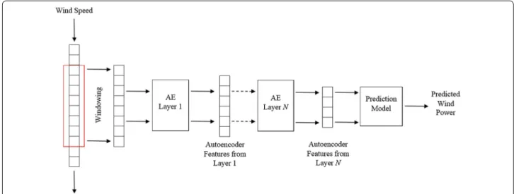
We have utilised a SAE to obtain the structural features
from the different stages, which are then used as the
fea-tures in the wind power prediction framework. The SAE
feature-based wind power prediction framework is
pre-sent in Fig. 1.
Cluster‑based ensemble prediction
Previous studies (Tasnim et al. 2014) indicate the
ensem-ble learning can improve prediction performance. In
addition to SAE features, we thus investigated how the
AE features perform in combination with ensemble
learning. Data suggest existence of natural clusters within
wind data, and we thus investigated cluster-based
ensem-ble learning in this regard. Cluster-based classification
was investigated previously in Verma and Rahman (2012),
and later adopted in Tasnim et al. (2017) as cluster-based
regression. The training and test workflow of
cluster-based ensemble regression
(CBER) for wind power
pre-diction are present in Figs. 2 and 3, respectively. Training
data (built on feature representation of wind speed data)
are clustered first, and regression models (mapping
functions) are trained on each cluster separately. When
predicting for test/new sample, the appropriate
(near-est) cluster is first found, and the regression model
cor-responding to that cluster maps the test sample to wind
power. We have investigated the influence of
incorporat-ing SAE features into CBER framework.
Fig. 1 Stacked autoencoder feature extraction for wind power prediction
Training Data Clustering
Data (Cluster 1)
•••
Data (Cluster 2)
Model Learning Regression Model (Cluster 1)
Model Learning
•••
Data (Cluster n) Model Learning
Regression Model (Cluster 2)
Regression Model (Cluster n)
Experimental setup
We have obtained historical wind speed data from
Bureau of Meteorology
(BoM) at 70 different stations
across Australia. A total of ten locations were selected
from each state randomly, and daily wind speed data
were collected for each location. The duration of the time
period varies between stations. A time window of 30 days
was used to extract wind speed records from historical
data, and 13 statistical features (“Statistical features”
sec-tion) were computed on each of these time windows. The
target for the vector was set to be day-ahead wind power.
We did not have any historical record of wind power
pro-duction. However, a power curve associated with a
tur-bine can provide a nonlinear transformation from wind
speed to power. We have utilised the power curve of
Sie-mens SWT–2.3 82 turbine (Staffell 2017) as used in
Tas-nim et al. (2014) to produce the corresponding power a
day ahead. The power curve for this turbine is present in
Fig. 4. We used 80% of the data for training and 20% for
testing. The best learning models were obtained from the
training data and applied on test data to compute
predic-tion accuracy. The performance reported here is based
on test set errors.
Given a window size of 30 for the time series data, we
developed a two-stage autoencoder with 25 hidden nodes
at stage 1 and 13 nodes at stage 2. Thus, the number of
features (i.e. activations) at stage 1 and 2 are 25 and 13,
respectively. The networks were trained for 100 and 50
iterations at stage 1 and stage 2, respectively. The desired
average activations were set to 0.01. The weight decay
parameter and sparsity penalty terms were set to zero.
The autoencoder was designed using the guidelines from
UFLDL Tutorial (2016). We have conducted the
experi-ments in MATLAB. We have utilised the linear
regres-sion implementations in MATLAB and LibSVM (Chang
and Lin 2011) implementation of the nonlinear SVM
(
support vector machine
) regression. We have used
k
-means clustering algorithm for the CBER framework. We
prepared the data set to forecast one-day-ahead power.
We assume that all the features are equally important
unlike feature selection methods (Rahman and Murshed
2004).
Results and discussion
The analysis on the performance of the SAE features for
wind power prediction is presented in this section. We
first compare the performance of SAE features at
dif-ferent stages. Given that the length of the input feature
space is only 30, we designed a two-stage SAE with the
first stage producing 25 (around 80% of length of input
vector) and the second stage producing 13 (around 50%
of the length of stage 1 SAE vector) structural features. If
additional stages are added with further reduction in
hid-den units, the feature space will be too small after that to
represent anything meaningful. Hence, we designed the
two-stage SAE. The regression errors produced on the 70
stations with SAE stage 1 and stage 2 structural features
using
linear regression
(LR) and SVM regression methods
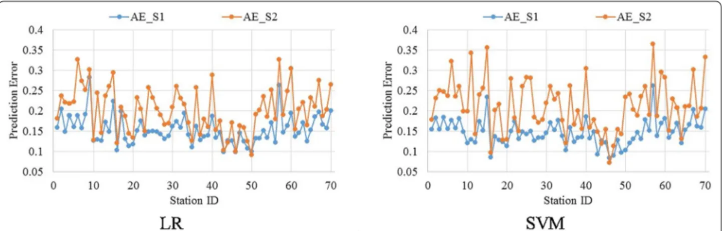
are present in Fig. 5. Stage 1 SAE features perform better
than stage 2 SAE features on 68 out of 70 stations using
both LR and SVM. This suggests that stage 1 SAE features
capture the structure of the underlying time series better
than stage 2 SAE features. On an average, the regression
error with stage 1 SAE features 4.91% lower than that of
stage 2 SAE features.
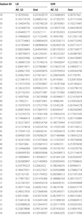
The prediction performance of SAE features to that of
statistical features is compared next in Figs. 6 and 7.
Stage
1 (S1) and
stage
2 (S2) SAE features perform better than
statistical features on 59 and 52 stations, respectively,
using LR. Similarly, SAE S1 and S2 features outperform
statistical features on 68 and 61 stations, respectively,
using SVM regression. This implies SAE structural
fea-tures are more suitable for regression compared to
struc-tural features. On an average, SAE S1 features perform
8.57 and 12.63% better than statistical features using LR
Test sample Find nearest cluster cluster kNearest Regression Model (Cluster k) Wind Power PredictedFig. 3 Testing model for cluster-based regression
and SVM regression, respectively. Similarly, SAE S2
fea-tures perform better than statistical feafea-tures by 3.66 and
6.05% using LR and SVM regression, respectively.
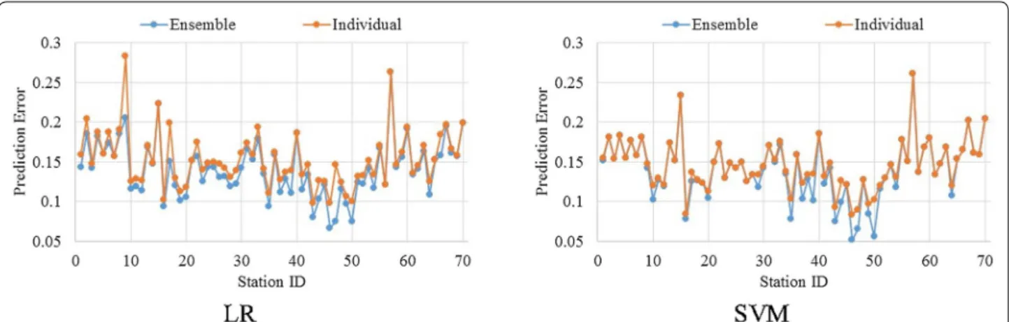
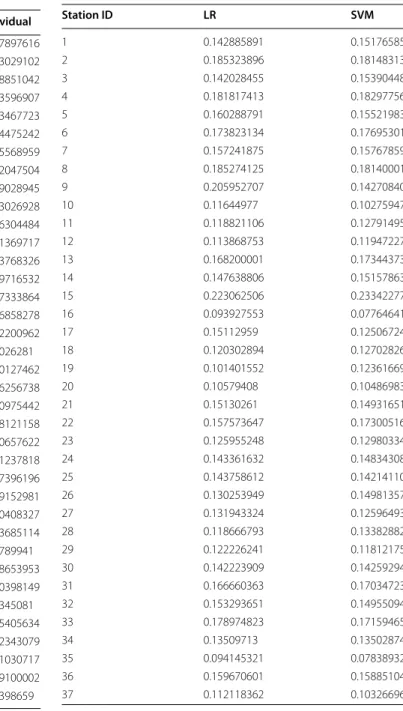
Next we investigated the performance of SAE
fea-tures as part of the CBER framework discussed in
“Cluster-based ensemble prediction” section. CBER
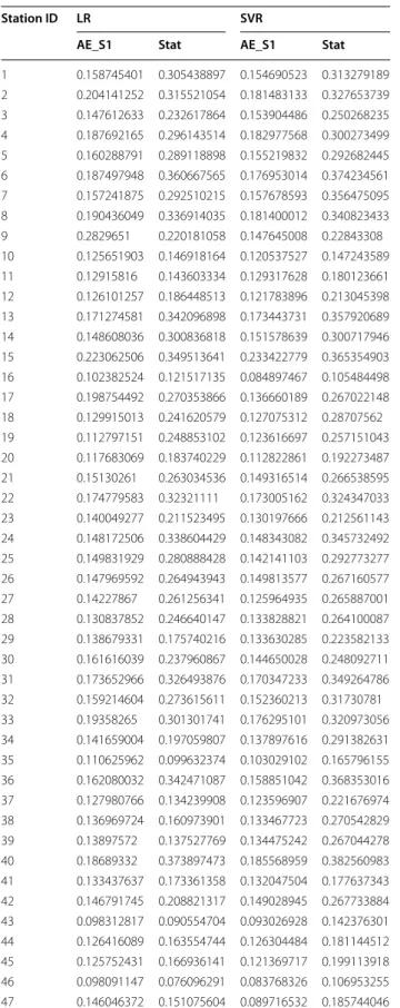
Fig. 5 Comparison of day-ahead prediction error between stage 1 and stage 2 AE features. Table 1 in appendix details the empirical resultsFig. 6 Comparison of day-ahead prediction error between SAE stage 1 and stat features. Table 2 in appendix details the empirical results
is formulated on incorporation of the natural groups
within data into the learning process. Figure
8
pre-sents the performance of SAE features as part of CBER
(ensemble) framework and when used individually
without any ensemble model. The CBER either
per-forms better than individual or equally in all 70 stations
using LR and SVR. On an average, CBER performs 1.20
and 0.53% better than the base (i.e. individual) learner
using LR and SVR, respectively. The improvement,
however, is very little and this implies CBER framework
has little influence on improving the performance of
SAE features. Finally, we compared the performance of
LR and SVR with SAE features in Fig.
9. LR performs
better than SVR on 37 occasions. Realistically there is
no significant difference between them. This implies
linear regression (LR) suits well for some stations
whereas nonlinear regression (SVR) suits well for some
stations.
Conclusion
In this paper, an algorithm for wind power prediction
is presented using autoencoder. A two-stage stacked
autoencoder (a particular type of deep learning) is
designed to produce structural features and incorporate
them into different learning frameworks for predicting
wind power. The performance of SAE features is also
compared with commonly used statistical features. Then,
we investigated how well the SAE features integrate with
cluster-based ensemble regression. Experiments were
conducted on 70 sites across the different states of
Aus-tralia. Following are the findings: (1) Stage 1 SAE features
perform better than the following stages. This is because
of a small number of features at later stages that fail to
appropriately capture the structure of the data, (2) SAE
features perform as high as 12.63% better than
statisti-cal features; however, the performance depends on the
usage of underlying learning algorithm, (3) Incorporation
of SAE features in CBER framework improves the
pre-diction performance; however, the improvement is very
little, and (4) Choice of linear or nonlinear regression
algorithm with SAE features depends on the data
charac-teristics of the station as there was not a clear winner. In
Fig. 8 Comparison of day-ahead prediction error between ensemble and individual classifier. Table 4 in appendix details the empirical resultsfuture, we aim to investigate other variants of deep
learn-ing algorithms to improve prediction accuracy of wind
power.
Authors’ contributions
All the authors made their contributions to the research and paper. The order-ing of the authors is as follows based on their contribution: ST, AR, AMTO, and MEH. All authors read and approved the final manuscript.
Author details
1 School of Engineering, Deakin University, Victoria, Australia. 2 Data61, CSIRO,
15 College Rd, Sandy Bay, TAS 7005, Australia.
Competing interests
The authors declare that they have no competing interests.
Availability of data and materials
The data are all publicly available.
Consent for publication
Not applicable.
Ethics approval and consent to participate
Not applicable.
Appendix
See Tables 1, 2, 3, 4, and 5.
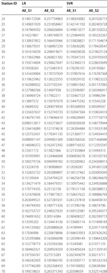
Table 1 Comparison of day-ahead prediction error between stage 1 and stage 2 AE features
Station ID LR SVR
AE_S1 AE_S2 AE_S1 AE_S2
1 0.158745401 0.181067965 0.154690523 0.177423941 2 0.204141252 0.236586197 0.181483133 0.231462248 3 0.147612633 0.220896913 0.153904486 0.250154358 4 0.187692165 0.217901965 0.182977568 0.246349006 5 0.160288791 0.222259356 0.155219832 0.236832626 6 0.187497948 0.32668499 0.176953014 0.322644395 7 0.157241875 0.273802047 0.157678593 0.235272042 8 0.190436049 0.251920268 0.181400012 0.259831581 9 0.2829651 0.301258024 0.147645008 0.198925306 10 0.125651903 0.128087603 0.120537527 0.198115693 11 0.12915816 0.243545578 0.129317628 0.343275183 12 0.126101257 0.144885552 0.121783896 0.142497862 13 0.171274581 0.236947145 0.173443731 0.240068251 14 0.148608036 0.259797678 0.151578639 0.255632804 15 0.223062506 0.294437347 0.233422779 0.356264684 16 0.102382524 0.120315586 0.084897467 0.097409784 17 0.198754492 0.209187753 0.136660189 0.200789565 18 0.129915013 0.18705036 0.127075312 0.216086943 19 0.112797151 0.143174729 0.123616697 0.127202701 20 0.117683069 0.134034792 0.112822861 0.128793831 21 0.15130261 0.232400756 0.149316514 0.278975728 22 0.174779583 0.204405777 0.173005162 0.181932923 23 0.140049277 0.149666039 0.130197666 0.14941992
Table 1 continued
Station ID LR SVR
AE_S1 AE_S2 AE_S1 AE_S2
Table 2 Comparison of day-ahead prediction error between SAE stage 1 and stat features
Station ID LR SVR
AE_S1 Stat AE_S1 Stat
1 0.158745401 0.305438897 0.154690523 0.313279189 2 0.204141252 0.315521054 0.181483133 0.327653739 3 0.147612633 0.232617864 0.153904486 0.250268235 4 0.187692165 0.296143514 0.182977568 0.300273499 5 0.160288791 0.289118898 0.155219832 0.292682445 6 0.187497948 0.360667565 0.176953014 0.374234561 7 0.157241875 0.292510215 0.157678593 0.356475095 8 0.190436049 0.336914035 0.181400012 0.340823433 9 0.2829651 0.220181058 0.147645008 0.22843308 10 0.125651903 0.146918164 0.120537527 0.147243589 11 0.12915816 0.143603334 0.129317628 0.180123661 12 0.126101257 0.186448513 0.121783896 0.213045398 13 0.171274581 0.342096898 0.173443731 0.357920689 14 0.148608036 0.300836818 0.151578639 0.300717946 15 0.223062506 0.349513641 0.233422779 0.365354903 16 0.102382524 0.121517135 0.084897467 0.105484498 17 0.198754492 0.270353866 0.136660189 0.267022148 18 0.129915013 0.241620579 0.127075312 0.28707562 19 0.112797151 0.248853102 0.123616697 0.257151043 20 0.117683069 0.183740229 0.112822861 0.192273487 21 0.15130261 0.263034536 0.149316514 0.266538595 22 0.174779583 0.32321111 0.173005162 0.324347033 23 0.140049277 0.211523495 0.130197666 0.212561143 24 0.148172506 0.338604429 0.148343082 0.345732492 25 0.149831929 0.280888428 0.142141103 0.292773277 26 0.147969592 0.264943943 0.149813577 0.267160577 27 0.14227867 0.261256341 0.125964935 0.265887001 28 0.130837852 0.246640147 0.133828821 0.264100087 29 0.138679331 0.175740216 0.133630285 0.223582133 30 0.161616039 0.237960867 0.144650028 0.248092711 31 0.173652966 0.326493876 0.170347233 0.349264786 32 0.159214604 0.273615611 0.152360213 0.31730781 33 0.19358265 0.301301741 0.176295101 0.320973056 34 0.141659004 0.197059807 0.137897616 0.291382631 35 0.110625962 0.099632374 0.103029102 0.165796155 36 0.162080032 0.342471087 0.158851042 0.368353016 37 0.127980766 0.134239908 0.123596907 0.221676974 38 0.136969724 0.160973901 0.133467723 0.270542829 39 0.13897572 0.137527769 0.134475242 0.267044278 40 0.18689332 0.373897473 0.185568959 0.382560983 41 0.133437637 0.173361358 0.132047504 0.177637343 42 0.146791745 0.208821317 0.149028945 0.267733884 43 0.098312817 0.090554704 0.093026928 0.142376301 44 0.126416089 0.163554744 0.126304484 0.181144512 45 0.125752431 0.166936141 0.121369717 0.199113918 46 0.098091147 0.076096291 0.083768326 0.106953255 47 0.146046372 0.151075604 0.089716532 0.185744046
Table 2 continued
Station ID LR SVR
AE_S1 Stat AE_S1 Stat
48 0.12421172 0.252681913 0.127333864 0.257876938 49 0.107059991 0.097565806 0.096858278 0.143250756 50 0.100279726 0.080950048 0.102200962 0.231154676 51 0.13224318 0.130506317 0.12026281 0.263569207 52 0.132825722 0.221409903 0.130127462 0.275908642 53 0.15139564 0.22662422 0.146256738 0.30946615 54 0.134271479 0.142527627 0.130975442 0.276862718 55 0.170774335 0.321793922 0.178121158 0.327291203 56 0.121676858 0.231476306 0.150657622 0.285133377 57 0.263049521 0.383450318 0.261237818 0.393449808 58 0.146794392 0.260921452 0.137396196 0.304257779 59 0.162753727 0.272668566 0.169152981 0.292383189 60 0.194091652 0.352073594 0.180408327 0.360152467 61 0.13595202 0.163491438 0.133685114 0.295869513 62 0.145129362 0.215443473 0.14789941 0.292035302 63 0.17036906 0.299126749 0.168653953 0.318091952 64 0.125395886 0.120358507 0.120398149 0.245715996 65 0.152778773 0.301768873 0.15345081 0.307462709 66 0.184463321 0.286654162 0.165405634 0.288571711 67 0.197356767 0.335890323 0.202343079 0.354104682 68 0.166242503 0.279201159 0.161030717 0.285498969 69 0.157746289 0.241333179 0.159100002 0.244219105 70 0.199218631 0.346426496 0.20398659 0.358764236
Table 3 Comparison of day-ahead prediction error between SAE stage 2 and stat features
Station ID LR SVR
AE_S2 Stat AE_S2 Stat
Table 3 continued
Station ID LR SVR
AE_S2 Stat AE_S2 Stat 18 0.18705036 0.241620579 0.216086943 0.28707562 19 0.143174729 0.248853102 0.127202701 0.257151043 20 0.134034792 0.183740229 0.128793831 0.192273487 21 0.232400756 0.263034536 0.278975728 0.266538595 22 0.204405777 0.32321111 0.181932923 0.324347033 23 0.149666039 0.211523495 0.14941992 0.212561143 24 0.257734863 0.338604429 0.261026715 0.345732492 25 0.231858467 0.280888428 0.282403728 0.292773277 26 0.206026804 0.264943943 0.281550252 0.267160577 27 0.189749075 0.261256341 0.183232267 0.265887001 28 0.166435966 0.246640147 0.171104674 0.264100087 29 0.168907239 0.175740216 0.178428547 0.223582133 30 0.208419671 0.237960867 0.219625124 0.248092711 31 0.260821392 0.326493876 0.259705033 0.349264786 32 0.230627647 0.273615611 0.228635699 0.31730781 33 0.215481915 0.301301741 0.24195061 0.320973056 34 0.170737039 0.197059807 0.176787368 0.291382631 35 0.126222555 0.099632374 0.119823225 0.165796155 36 0.257102341 0.342471087 0.261737082 0.368353016 37 0.14097938 0.134239908 0.165996917 0.221676974 38 0.17902211 0.160973901 0.19986294 0.270542829 39 0.159707679 0.137527769 0.15545228 0.267044278 40 0.289074934 0.373897473 0.30509547 0.382560983 41 0.152743733 0.173361358 0.159024316 0.177637343 42 0.174696419 0.208821317 0.177718773 0.267733884 43 0.102273657 0.090554704 0.148770944 0.142376301 44 0.121374618 0.163554744 0.119333189 0.181144512 45 0.170341135 0.166936141 0.154934419 0.199113918 46 0.099001309 0.076096291 0.071468486 0.106953255 47 0.162472392 0.151075604 0.112355547 0.185744046 48 0.15821066 0.252681913 0.15494315 0.257876938 49 0.124466068 0.097565806 0.143105742 0.143250756 50 0.090999782 0.080950048 0.234308913 0.231154676 51 0.190908691 0.130506317 0.241601228 0.263569207 52 0.202089897 0.221409903 0.203005045 0.275908642 53 0.234794223 0.22662422 0.188246676 0.30946615 54 0.184479351 0.142527627 0.234926888 0.276862718 55 0.25132158 0.321793922 0.260388512 0.327291203 56 0.179877821 0.231476306 0.188886769 0.285133377 57 0.327281031 0.383450318 0.364458141 0.393449808 58 0.189771426 0.260921452 0.18674796 0.304257779 59 0.248327635 0.272668566 0.295240371 0.292383189 60 0.30514384 0.352073594 0.282399715 0.360152467 61 0.154414136 0.163491438 0.151898183 0.295869513 62 0.203880626 0.215443473 0.229171978 0.292035302 63 0.220678896 0.299126749 0.207426242 0.318091952 64 0.165066098 0.120358507 0.130643205 0.245715996
Table 4 Comparison of day-ahead prediction error between ensemble and individual classifier
Station ID LR SVR
Ensemble Individual Ensemble Individual
1 0.142885891 0.158745401 0.151765852 0.154690523 2 0.185323896 0.204141252 0.181483133 0.181483133 3 0.142028455 0.147612633 0.153904486 0.153904486 4 0.181817413 0.187692165 0.182977568 0.182977568 5 0.160288791 0.160288791 0.155219832 0.155219832 6 0.173823134 0.187497948 0.176953014 0.176953014 7 0.157241875 0.157241875 0.157678593 0.157678593 8 0.185274125 0.190436049 0.181400012 0.181400012 9 0.205952707 0.2829651 0.142708409 0.147645008 10 0.11644977 0.125651903 0.102759471 0.120537527 11 0.118821106 0.12915816 0.127914958 0.129317628 12 0.113868753 0.126101257 0.119472275 0.121783896 13 0.168200001 0.171274581 0.173443731 0.173443731 14 0.147638806 0.148608036 0.151578639 0.151578639 15 0.223062506 0.223062506 0.233422779 0.233422779 16 0.093927553 0.102382524 0.077646418 0.084897467 17 0.15112959 0.198754492 0.125067241 0.136660189 18 0.120302894 0.129915013 0.127028267 0.127075312 19 0.101401552 0.112797151 0.123616697 0.123616697 20 0.10579408 0.117683069 0.104869831 0.112822861 21 0.15130261 0.15130261 0.149316514 0.149316514 22 0.157573647 0.174779583 0.173005162 0.173005162 23 0.125955248 0.140049277 0.129803347 0.130197666 24 0.143361632 0.148172506 0.148343082 0.148343082 25 0.143758612 0.149831929 0.142141103 0.142141103 26 0.130253949 0.147969592 0.149813577 0.149813577 27 0.131943324 0.14227867 0.125964935 0.125964935 28 0.118666793 0.130837852 0.133828821 0.133828821 29 0.122226241 0.138679331 0.118121759 0.133630285 30 0.142223909 0.161616039 0.142592948 0.144650028 31 0.166660363 0.173652966 0.170347233 0.170347233 32 0.153293651 0.159214604 0.149550942 0.152360213 33 0.178974823 0.19358265 0.171594656 0.176295101 Station ID LR SVR
AE_S2 Stat AE_S2 Stat
65 0.232503266 0.301768873 0.21071125 0.307462709 66 0.209924359 0.286654162 0.211359147 0.288571711 67 0.27515283 0.335890323 0.30213711 0.354104682 68 0.185966745 0.279201159 0.185332165 0.285498969 69 0.202268433 0.241333179 0.20638384 0.244219105 70 0.265371343 0.346426496 0.332514288 0.358764236
Table 4 continued
Station ID LR SVR
Ensemble Individual Ensemble Individual 34 0.13509713 0.141659004 0.135028746 0.137897616 35 0.094145321 0.110625962 0.078389329 0.103029102 36 0.159670601 0.162080032 0.158851042 0.158851042 37 0.112118362 0.127980766 0.103266967 0.123596907 38 0.12829815 0.136969724 0.129128618 0.133467723 39 0.11058723 0.13897572 0.10147942 0.134475242 40 0.18610048 0.18689332 0.185568959 0.185568959 41 0.115441421 0.133437637 0.122019194 0.132047504 42 0.133978696 0.146791745 0.141909547 0.149028945 43 0.080612644 0.098312817 0.075334057 0.093026928 44 0.103591698 0.126416089 0.098886049 0.126304484 45 0.120956411 0.125752431 0.121369717 0.121369717 46 0.066782811 0.098091147 0.051633227 0.083768326 47 0.074709577 0.146046372 0.065871144 0.089716532 48 0.116237973 0.12421172 0.127333864 0.127333864 49 0.097123426 0.107059991 0.08476987 0.096858278 50 0.074662291 0.100279726 0.056369624 0.102200962 51 0.124928262 0.13224318 0.115692258 0.12026281 52 0.12260507 0.132825722 0.130127462 0.130127462 53 0.141934357 0.15139564 0.146256738 0.146256738 54 0.117538787 0.134271479 0.117826505 0.130975442 55 0.167406487 0.170774335 0.178121158 0.178121158 56 0.121676858 0.121676858 0.150657622 0.150657622 57 0.263049521 0.263049521 0.261237818 0.261237818 58 0.143628828 0.146794392 0.137061915 0.137396196 59 0.155726183 0.162753727 0.169152981 0.169152981 60 0.191407122 0.194091652 0.180408327 0.180408327 61 0.134242101 0.13595202 0.133685114 0.133685114 62 0.140952265 0.145129362 0.14789941 0.14789941 63 0.16355478 0.17036906 0.168653953 0.168653953 64 0.108631779 0.125395886 0.108052209 0.120398149 65 0.152778773 0.152778773 0.15345081 0.15345081 66 0.157908601 0.184463321 0.165405634 0.165405634 67 0.195097256 0.197356767 0.202343079 0.202343079 68 0.161617909 0.166242503 0.161030717 0.161030717 69 0.157390727 0.157746289 0.159100002 0.159100002 70 0.199218631 0.199218631 0.20398659 0.20398659
Table 5 Comparison of day-ahead prediction error between LR and SVM using CBER
Station ID LR SVM
1 0.142885891 0.151765852
2 0.185323896 0.181483133
3 0.142028455 0.153904486
4 0.181817413 0.182977568
5 0.160288791 0.155219832
6 0.173823134 0.176953014
7 0.157241875 0.157678593
8 0.185274125 0.181400012
9 0.205952707 0.142708409
10 0.11644977 0.102759471
11 0.118821106 0.127914958
12 0.113868753 0.119472275
13 0.168200001 0.173443731
14 0.147638806 0.151578639
15 0.223062506 0.233422779
16 0.093927553 0.077646418
17 0.15112959 0.125067241
18 0.120302894 0.127028267
19 0.101401552 0.123616697
20 0.10579408 0.104869831
21 0.15130261 0.149316514
22 0.157573647 0.173005162
23 0.125955248 0.129803347
24 0.143361632 0.148343082
25 0.143758612 0.142141103
26 0.130253949 0.149813577
27 0.131943324 0.125964935
28 0.118666793 0.133828821
29 0.122226241 0.118121759
30 0.142223909 0.142592948
31 0.166660363 0.170347233
32 0.153293651 0.149550942
33 0.178974823 0.171594656
34 0.13509713 0.135028746
35 0.094145321 0.078389329
36 0.159670601 0.158851042
Publisher’s Note
Springer Nature remains neutral with regard to jurisdictional claims in pub-lished maps and institutional affiliations.
Received: 8 August 2017 Accepted: 4 December 2017
References
Bengio, Y., Lamblin, P., Popovici, D., & Larochelle, H. (2007). Greedy layer-wise training of deep networks. In B. Scholkopf, J. Platt, & T. Hoffman (Eds.), Advances in neural information processing systems 19 (NIPS’06) (pp. 153–160). Cambridge: MIT Press.
Chang, C.-C., & Lin, C.-J. (2011). LIBSVM: A library for support vector machines. ACM Transactions on Intelligent Systems and Technology, 2, 27:1–27:27. Colak, I., Sagiroglu, S., & Yesilbudak, M. (2012). Data mining and wind power
prediction: A literature review. Renewable Energy, 46, 241–247.
Gehrig, J., Miao, Y., Metze, F., & Waibel, A. (2013). Extracting deep bottleneck features using stacked auto-encoders. In Proceedings of IEEE international conference on acoustics, audio and speech (pp. 3371–3381). Vancouver. IRENA. (2017). Renewable energy integration in power grids. http://www.irena.
org/menu/index.aspx?mnu=Subcat&PriMenuID=36&CatID=141&Subca tID=644. Last accessed August 2017.
Jiang, P., Liu, F., & Song, Y. (2017). A hybrid forecasting model based on date-framework strategy and improved feature selection technology for short-term load forecasting. Energy 119, 694–709, ISSN 0360-5442. https:// doi.org/10.1016/j.energy.2016.11.034.
Ng, A. (2016). Sparse autoencoder (pp. 1–19). http://web.stanford.edu/class/ cs294a/sae/sparseAutoencoderNotes.pdf. Last accessed January 2016. Rahman, A., & Murshed, M. (2004). Feature weighting methods for abstract features applicable to motion based video indexing. In IEEE international conference on information technology: Coding and computing (ITCC) (Vol. 1, pp. 676–680).
Rahman, A., Smith, D., Hills, J., Bishop-Hurley, G., Henry, D., & Rawnsley, R. (2016). A comparison of autoencoder and statistical features for cattle behaviour classification. In 2016 international joint conference on neural networks (IJCNN) (pp. 2954–2960). Vancouver. https://doi.org/10.1109/ ijcnn.2016.7727573.
Rahman, A., & Verma, B. (2010). A novel ensemble classifier approach using weak classifier learning on overlapping clusters. In The 2010 international joint conference on neural networks (IJCNN) (pp. 1–7). Barcelona. https:// doi.org/10.1109/ijcnn.2010.5596332
Rahman, A., & Verma, B. (2011). Novel layered clustering-based approach for generating ensemble of classifiers. IEEE Transactions on Neural Networks, 22(5), 781–792. https://doi.org/10.1109/TNN.2011.2118765.
Shin, H., Orton, M., Collins, D. J., Doran, S., & Leach, M. O. (2011). Autoencoder in time-series analysis for unsupervised tissues characterisation in a large unlabelled medical image data set. In Proceedings of IEEE international conference on machine learning and application (pp. 259–264).
Shin, H.-C., Orton, M. R., Collins, D. J., Doran, S. J., & Leach, M. O. (2014). Stacked autoencoders for unsupervised feature learning and multiple organ detection in a pilot study using 4D patient data. IEEE Transactions on Pat-tern Analysis and Machine Intelligence, 8(35), 1930–1943.
Soman, S. S., Zareipour, H., Malik, O., & Mandal, P. (2010). A review of wind power and wind speed forecasting methods with different time hori-zons. North American Power Symposium (NAPS), 2010, 1–8. https://doi. org/10.1109/NAPS.2010.5619586.
Staffell. (2017). Wind turbine power curves. http://www.academia.edu/1489838/ Wind_Turbine_Power_Curves. Last accessed August 2017.
Tasnim, S., Rahman, A., Shafiullah, G. M., Oo, A. M. T., & Stojcevski, A. (2014). A time series ensemble method to predict wind power. In 2014 IEEE sympo-sium on computational intelligence applications in smart grid (CIASG) (pp. 1–5), Orlando, FL. https://doi.org/10.1109/ciasg.2014.7011544
Tasnim, S., Rahman, A., Oo, A. M. T., & Haque, M. E. (2017). Wind power predic-tion using cluster based ensemble regression. Internapredic-tional Journal of Computational Intelligence and Applications. https://doi.org/10.1142/ S1469026817500262.
UFLDL Tutorial. (2016). Sparse autoencoder. http://deeplearning.stanford.edu/ wiki/index.php/UFLDL_Tutorial. Last accessed January 2016.
Verma, B., & Rahman, A. (2012). Cluster-oriented ensemble classifier: Impact of multicluster characterization on ensemble classifier learning. IEEE Transactions on Knowledge and Data Engineering, 24(4), 605–618. https:// doi.org/10.1109/TKDE.2011.28.
Vincent, P., Larochelle, H., Lajoie, I., Bengio, Y., & Manjagol, P. A. (2010). Stacked denoising autoencoders: Learning useful representations in a deep net-work with a local denoising criteria. Journal of Machine Learning Research, 11, 3371–3408.
Wang, X., Guo, P., & Huang, X. (2011). A review of wind power forecasting models. Energy Procedia, 12, 770–778.
Wang, J., Song, Y., Liu, F., & Hou, R. (2016). Analysis and application of forecasting models in wind power integration: A review of multi-step-ahead wind speed forecasting models. Renewable and Sustainable Energy Reviews 60, 960–981, ISSN 1364-0321. https://doi.org/10.1016/j. rser.2016.01.114.
Zhao, J., Guo, Z.-H., Su, Z.-Y., Zhao, Z.-Y., Xiao, X., & Liu, F. (2016). An improved multi-step forecasting model based on WRF ensembles and creative fuzzy systems for wind speed. Applied Energy 162, 808–826, ISSN 0306-2619. https://doi.org/10.1016/j.apenergy.2015.10.145.
Table 5 continued
Station ID LR SVM
38 0.12829815 0.129128618
39 0.11058723 0.10147942
40 0.18610048 0.185568959
41 0.115441421 0.122019194
42 0.133978696 0.141909547
43 0.080612644 0.075334057
44 0.103591698 0.098886049
45 0.120956411 0.121369717
46 0.066782811 0.051633227
47 0.074709577 0.065871144
48 0.116237973 0.127333864
49 0.097123426 0.08476987
50 0.074662291 0.056369624
51 0.124928262 0.115692258
52 0.12260507 0.130127462
53 0.141934357 0.146256738
54 0.117538787 0.117826505
55 0.167406487 0.178121158
56 0.121676858 0.150657622
57 0.263049521 0.261237818
58 0.143628828 0.137061915
59 0.155726183 0.169152981
60 0.191407122 0.180408327
61 0.134242101 0.133685114
62 0.140952265 0.14789941
63 0.16355478 0.168653953
64 0.108631779 0.108052209
65 0.152778773 0.15345081
66 0.157908601 0.165405634
67 0.195097256 0.202343079
68 0.161617909 0.161030717
69 0.157390727 0.159100002