ISSN 2307-7743 http://scienceasia.asia
ON A GENERALIZED SIGMOID FUNCTION AND ITS PROPERTIES
K. NANTOMAH1,∗, C. A. OKPOTI2 AND S. NASIRU3
1 Department of Mathematics, Faculty of Mathematical Sciences, University for
Development Studies, Navrongo Campus, P. O. Box 24, Navrongo, UE/R, Ghana
2 Department of Mathematics, University of Education, Winneba, Ghana
3 Department of Statistics, Faculty of Mathematical Sciences, University for Development
Studies, Navrongo Campus, P. O. Box 24, Navrongo, UE/R, Ghana
∗Correspondence: [email protected]
Abstract. Motivated by generalized forms of the exponential and hyperbolic functions,
we introduce a new generalization of the sigmoid function and further study some of its
analytical properties.
1. Introduction
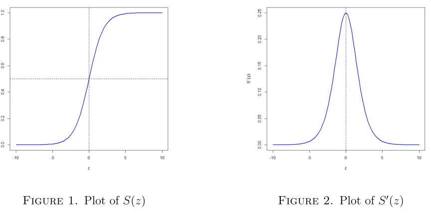
The sigmoid function, which is otherwise known as the standard logistic function is defined for z ∈R= (−∞,∞) as
S(z) = e
z
1 +ez =
1 1 +e−z
(1)
= 1 2+
1 2tanh
z
2
. (2)
It is monotone increasing and its first derivative is bell-shaped. See the plots below.
This special function is applied in many scientific disciplines such as machine learning, artificial neural networks, computer graphics, medicine, probability and statistics, biology, ecology, population dynamics, demography, and mathematical psychology. See for instance [1], [2], [3], [4], [5], [6], [8], [10], [11], [12], [13], and the several related references therein. Due to the important roles of this function, recent works have focused on investigating its analytical properties. In [9], the authors studied properties of the function such as starlikeness and convexity in a unit disc. In [14], the author studied among other things
Keywords: Generalized exponential function; generalized hyperbolic functions; generalized sigmoid
func-tion; generalized softplus funcfunc-tion; inequality.
c
2020 Science Asia
Figure 1. Plot of S(z) Figure 2. Plot of S0(z)
some properties such as subadditivity, log-concavity, monotonicity and geometric concavity of the function. Thereafter, in [17], the authors introduced a generalization of the function and by adopting the techniques of [14], they proved analogous properties for the generalized function. They also considered some statistical properties of the generalized function.
Motivated by generalized forms of the exponential and hyperbolic functions, the goal of this paper is to introduce a new generalization of the sigmoid function and to further study some of its analytical properties.
Definition 1.1 ([16]). Let φ :I ⊆ R+ = (0,∞)→
R+. Then φ is said to be geometrically convex on I if
(3) φ xry1−r ≤[φ(x)]r[φ(y)]1−r
for all x, y ∈ I and r ∈ [0,1]. If the inequality in (3) is reversed, then φ is said to be geometrically concave on I.
Lemma 1.2 ([15]). Let φ : I ⊆ R+ →
R+ be a differentiable function. Then the following statements are equivalent.
(a) The function φ is geometrically convex (concave). (b) The function zφφ(0z(z)) is increasing (decreasing).
2. Generalized Sigmoid Function and its Properties
Definition 2.1. Leta >1. Then the generalized exponential function is defined as
(4) az =
∞
X
n=0
(lna)nzn
n! ,
for all z ∈R.
From this definition, we define the generalized hyperbolic cosine, hyperbolic sine and hyperbolic tangent functions as follows.
Definition 2.2. Let a > 1. Then the generalized hyperbolic cosine, hyperbolic sine and hyperbolic tangent functions are respectively defined as
(5) cosha(z) =
az+a−z
2 ,
(6) sinha(z) =
az−a−z
2 ,
(7) tanha(z) =
sinha(z)
cosha(z)
= a
z−a−z
az+a−z = 1−
2 1 +a2z,
for all z ∈R.
These generalized functions satisfy the following identities.
(8) cosha(z) + sinha(z) = az,
(9) cosha(z)−sinha(z) =a−z,
(10) (cosha(z))
0
= (lna) sinha(z),
(11) (sinha(z))
0
= (lna) cosha(z),
(12) (tanha(z))
0
= lna cosh2a(z),
(13) (cosha(z))
00
+ (sinha(z)) 00
= (lna)2az,
(14) (cosha(z))
00
−(sinha(z)) 00
= (lna)2a−z,
(15) cosh2a(z) + sinh2a(z) = cosha(2z),
(16) cosh2a(z)−sinh2a(z) = 1.
Definition 2.3. Leta >1. Then the generalized sigmoid function is defined as Sa(z) =
az
1 +az,
(17)
= 1 2+
1 2tanha
z
2
, (18)
for all z ∈R. Clearly, when a=e, then Sa(z) reduces toS(z).
Direct computations reveals that this special function satisfies the following properties. Sa0(z) = (lna) a
z
(1 +az)2 = (lna)Sa(z) (1−Sa(z)), (19)
Sa00(z) = (lna)2a
z(1−az)
(1 +az)3 = (lna) 2S
a(z)(1−Sa(z))(1−2Sa(z)),
(20)
(21) (lnSa(z))
00
+ (lna)Sa0(z) = 0,
(22) Sa(z) = 1−Sa(−z),
(23) Sa0(z) = (lna)Sa(z)Sa(−z),
(24) lim
z→∞Sa(z) = 1,
(25) lim
z→0Sa(z) = 1 2,
(26) lim
z→−∞Sa(z) = 0,
(27) lim
z→±∞S 0
a(z) = 0,
(28) lim
z→0S
0 a(z) =
lna 4 ,
(29)
Z
Sa(z)dz =
ln(1 +az)
lna +k,
where k is a constant of integration. The function ln(1+lnaaz) is a generalization of the softplus function which was first defined in [7].
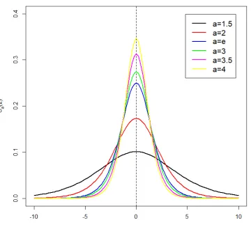
Remark 2.4. Figure 3 and Figure 4 respectively show the plots of the generalized sigmoid function and its derivative for some particular values of a. It is evident that the shapes of these functions depend on the values of a. The maximum value ofSa0(z) is ln4a for any a >1.
Remark 2.5. The function Sa(z) is a cumulative distribution function in the sense that:
(a) limz→−∞Sa(z) = 0,
(b) limz→∞Sa(z) = 1,
Figure 3. Plot of Sa(z) Figure 4. Plot of Sa0(z)
(d) Sa(z) is right-continuous.
The function Sa0(z) is the associated probability density function.
Theorem 2.6. The generalized sigmoid function satisfies the inequality
(30) Sa(w+z)< Sa(w) +Sa(z),
for all w, z ∈R. That is, Sa(z) is subadditive on R.
Proof. Let ψ(t) = 1+tt where t > 0. Then ψ(t) is strictly increasing for all t > 0. Also, let w, z ∈R. Then,
Sa(w) +Sa(z) =
aw
1 +aw +
az
1 +az =
aw+az+ 2aw+z
1 +aw+az+aw+z
> a
w+az+aw+z
1 +aw+az+aw+z
=ψ(aw+az+aw+z) > ψ(aw+z)
=Sa(w+z),
which gives the desired result.
Theorem 2.7. The generalized sigmoid function satisfies the inequality
(31) Sa(δw+ (1−δ)z)≥[Sa(w)]δ[Sa(z)]1−δ,
for all w, z ∈R and δ ∈[0,1]. That is, Sa(z) is logarithmically concave on R.
Proof. It suffices to show that (lnSa(z))00≤0 for all z ∈R. Let z ∈R. Then
(lnSa(z)) 00
=
Sa0(z) Sa(z)
0
= S
00
a(z)Sa(z)−(Sa0(z))2
[Sa(z)]2
=−(lna) 2az
which concludes the proof.
Remark 2.8. Theorem 2.7 is equivalent to the following statements. (a) Sa00(z)Sa(z)≤(Sa0(z))2 for all z∈R.
(b) Sa0(z)
Sa(z) is decreasing for all z ∈R.
Corollary 2.9. The inequality
(32) Sa(x)
Sa(x−1)
≥ Sa(x+ 1) Sa(x)
,
is satisfied for all x∈R.
Proof. By letting w=x−1, z =x+ 1 and δ= 12 in Theorem2.7, we obtain [Sa(x)]2 ≥Sa(x−1)Sa(x+ 1),
which yields inequality (32).
Theorem 2.10. The generalized sigmoid function satisfies the inequality
(33)
a 1 +a
1−λ
≤ [Sa(z+ 1)]
λ
Sa(λz+ 1)
≤1,
for z ∈(0,∞) and λ ≥1. The inequality is reversed if 0< λ≤1. Proof. Forz ∈(0,∞) and λ≥1, let β(z) = [Sa(z+1)]λ
Sa(λz+1) and h(z) = lnβ(z). Then
h0(z) = λ
Sa0(z+ 1) Sa(z+ 1)
− S
0
a(λz+ 1)
Sa(λz+ 1)
>0,
since S0a(z)
Sa(z) is decreasing. Thus, β(z) is increasing. Then for z ∈(0,∞), we have
f(0)≤β(z)≤ lim
z→∞β(z) = 1,
which yields inequality (33). The proof for the case where 0 < λ ≤ 1, follows a similar
procedure. Hence we omit the details.
Theorem 2.11. For α∈[0,1], the inequalities
(34) 1−α
2 ≤Sa(αz)−αSa(z)≤1−α, z ∈(0,∞),
(35) 0≤Sa(αz)−αSa(z)≤
1−α
2 , z ∈(−∞,0), are satisfied.
Proof. Note that
(Sa0(z))0 =Sa00(z) = (lna)2a
z(1−az)
respectively if z ∈ (−∞,0) or z ∈ (0,∞). Thus, Sa0(z) is increasing for z ∈ (−∞,0) and decreasing for z ∈ (0,∞). Let α ∈ [0,1] and φ(z) = Sa(αz)−αSa(z). Now suppose that
z ∈(0,∞). Then αz < z and then
φ0(z) =α[Sa0(αz)−Sa0(z)]>0,
since Sa0(z) is decreasing for z ∈(0,∞). Henceφ(z) is increasing for z ∈(0,∞). Therefore 1−α
2 =φ(0)≤φ(z)≤zlim→∞φ(z) = 1−α,
which gives (34). Next suppose thatz ∈(−∞,0). Then αz > z and φ0(z) =α[Sa0(αz)−Sa0(z)]>0,
since Sa0(z) is increasing for z ∈ (−∞,0). Henceφ(z) is increasing for z ∈(−∞,0) as well. Consequently
0 = lim
z→−∞φ(z)≤φ(z)≤φ(0) =
1−α 2 ,
which gives (35).
Remark 2.12. Inequalities (34) and (35) imply that Sa(αz)≥αSa(z) for all z ∈(−∞,∞)
and α∈[0,1]. In other words, the functionSa(z) is +∞-star-shaped. Theorem 2.13. The inequality
(36) (lna)Sa(x)<
ln(1 +az)−ln(1 +ax)
z−x <(lna)Sa(z), holds for 0≤x < z
Proof. Let 0≤x < z and consider the function γ(t) = ln(1 +at) on the interval (x, z). By
the mean value theorem, there exist a c∈(x, z) such that ln(1 +az)−ln(1 +ax)
z−x =γ
0
(c). Since γ0(t) = (lna)Sa(t) is increasing, then for c∈(x, z), we have
γ0(x)< γ0(c)< γ0(z),
which is equivalent to (36).
Remark 2.14. If x= 0 in Theorem 2.13, then we obtain
ln 2 + (lna)
2 z <ln(1 +a
z)<ln 2 + (lna)zS
a(z), z >0,
Theorem 2.15. Let r≥1. Then
(37)
Sa(x)
Sa(y)
r
≤ Sa(rx) Sa(ry)
,
if x≤y and
(38)
1 2
r−1
≤ [Sa(x)]
r
Sa(rx)
≤ 1 +a
r
(1 +a)r,
if x∈(0,1). Equality holds when r= 1. Proof. Letr ≥1, θ(x) = [Sa(x)]r
Sa(rx), and g(x) = lnθ(x). Then
g0(x) = r
Sa0(x) Sa(x)
− S
0 a(rx)
Sa(rx)
>0.
Thus,θ(x) is increasing. Then for x≤y, we have θ(x)≤θ(y),
which yields (37). Similarly for x∈(0,1), we have
1 2
r−1
= lim
x→0θ(x)≤θ(x)≤xlim→1θ(x) =
1 +ar
(1 +a)r,
which yields (38). This completes the proof.
Remark 2.16. If 0< r <1 in Theorem2.15, then we obtain the reverse cases of inequalities (37) and (38).
Theorem 2.17. The inequality
(39) Sa0 xλy1−λ≥[Sa0(x)]λ[Sa0(y)]1−λ, holds for x, y ∈R+ and λ∈[0,1]. That is, S0
a(z) is geometrically concave on R+.
Proof. Letz ∈R+. Then it follows from (19) and (20) that Sa00(z)
S0 a(z)
= (lna)1−a
z
1 +az,
and by direct computation, we obtain
zS
00 a(z)
S0 a(z)
0
= (lna)
1−az
1 +az −2(lna)
zaz
(1 +az)2
<0.
In view of Lemma 1.2, we conclude that Sa0(z) is geometrically concave on R+ and this is
Theorem 2.18. The inequalities
(40) 1< Sa(z+ 1)
Sa(z)
< a,
(41) 0< S
0 a(z)
Sa(z)
<lna,
hold for all z ∈R.
Proof. Let ∆(z) = Sa(z+1)
Sa(z) for all z ∈R. Then
lim
z→−∞∆(z) = limz→−∞
a+az+1 1 +az+1 =a and
lim
z→∞∆(z) = limz→∞
a+az+1 1 +az+1 = 1. Also,
∆0(z) ∆(z) =
Sa0(z+ 1) Sa(z+ 1)
− S
0 a(z)
Sa(z)
<0,
since S0a(z)
Sa(z) is decreasing. Thus, ∆(z) is decreasing. Hence for allz ∈R, we have
1 = lim
z→∞∆(z)<∆(z)<z→−∞lim ∆(z) =a,
which gives inequality (40). Next we have
lim
z→−∞
Sa0(z) Sa(z)
= lim
z→−∞
lna
1 +az = lna,
and
lim
z→∞
Sa0(z) Sa(z)
= lim
z→∞
lna 1 +az = 0.
Then by the monotonicity of Sa0(z)
Sa(z), we obtain
lim
z→∞
Sa0(z) Sa(z)
< S
0 a(z)
Sa(z)
< lim
z→−∞
Sa0(z) Sa(z)
,
which gives inequality (41).
Theorem 2.19. The inequalities
(42) 1
a <
Sa0(z+ 1) S0
a(z)
< a,
(43) −lna < S
00 a(z)
S0 a(z)
<lna,
Proof. Recall that Sa00(z)
S0
a(z) = (lna)
1−az
1+az for all z ∈R. Then
Sa00(z) S0
a(z)
0
=−2(lna)2 a
z
(1 +az)2 <0, which implies that Sa00(z)
S0
a(z) is decreasing. Also,
lim
z→−∞
Sa00(z) S0
a(z)
= lna and lim
z→∞
Sa00(z) S0
a(z)
=−lna.
Hence for z ∈R, we have
lim
z→∞
Sa00(z) S0 a(z) < S 00 a(z) S0 a(z) < lim z→−∞
Sa00(z) S0
a(z)
,
which gives inequality (43). Next, let D(z) = S0a(z+1)
S0
a(z) for all z ∈R. Then
lim
z→−∞D(z) = limz→−∞a
1 +az
1 +az+1
2
=a
and
lim
z→∞D(z) = limz→∞a
1 +az 1 +az+1
2
= 1 a.
In addition, we obtain
D0(z) D(z) =
Sa00(z+ 1) S0
a(z+ 1)
− S 00 a(z) S0 a(z) <0. Thus,D(z) is decreasing. Hence for all z ∈R, we have
1
a = limz→∞D(z)< D(z)<z→−∞lim D(z) = a,
which gives inequality (42).
Theorem 2.20. The inequalities
(44) a
1 +a ≤
Sa(x+ 1)Sa(y+ 1)
Sa(x+y+ 1)
<1,
holds for all x, y ∈[0,∞).
Proof. Letλ(x, y) = Sa(x+1)Sa(y+1)
Sa(x+y+1) for all x, y ∈[0,∞). Further let h(x, y) = lnλ(x, y). Then
∂
∂xh(x, y) =
Sa0(x+ 1) Sa(x+ 1)
− S
0
a(x+y+ 1)
Sa(x+y+ 1)
>0.
Thus,λ(x, y) is increasing. Hence a
1 +a = limx→0λ(x, y)≤λ(x, y)<xlim→∞λ(x, y) =Sa(y+ 1)<1,
3. Conclusion
In this work, we have introduced a new generalization of the sigmoid function which is frequently applied in machine learning, artificial neural networks, computer graphics, medicine, probability and statistics, biology, ecology, population dynamics, demography, and mathematical psychology. It is our fervent hope that, this new generalization and the properties established thereafter, will find useful applications in these scientific disciplines. We also anticipate that for some particular values of a, this generalized function may be applied in modeling datasets with heavy tails.
References
[1] P. BarrySigmoid functions and exponential Riordan arrays, arXiv:1702.04778v1 [math.CA]
[2] K. Basterretxea, J.M. Tarela and I. del Campo Approximation of sigmoid function and the derivative
for hardware implementation of artificial neurons, IEE Proc. Circuits Devices Syst. 151(1)(2004), 18-24.
[3] O. Centin, F. Temurtas and S. GulgonulAn application of multilayer neural network on hepatitis disease
diagnosis using approximations of sigmoid activation function, Dicle Med. J. 42(2)(2015), 150-157.
[4] Z. Chen and F. Cao The Approximation Operators with Sigmoidal Functions, Computer Math. Appl.
58(2009), 758-765.
[5] D. W. Coble and Y-J. Lee Use of a generalized Sigmoid Growth Function to predict Site Index for
Unmanaged Loblolly and Slash Pine Plantations in East Texas, USDA For. Serv., Gen. Tech. Rep.
SRS-92, Southern Research Station. Asheville, NC. P. 291295.
[6] B. Cyganek and K. SochaComputationally efficient methods of approximations of the S-shape functions
for Image Processing and Computer Graphics Tasks, Image Proc. Commun. 16(1-2)(2012), 19-28.
[7] C. Dugas, Y. Bengio, F. Belisle, C. Nadeau, and R. Garcia Incorporating second-order functional
knowledge for better option pricing, In Proceedings of NIPS 2001, Adv. Neural Inf. Proc. Syst. 14(2001),
472-478.
[8] D. Elliott A better activation function for artificial neural networks, The National Science Fondation,
Institute for Systems Research, Washington, DC, ISR Technical Rep. TR-6, 1993.
[9] U. A. Ezeafulukwe, M. Darus and O. Abidemi On Analytic Properties of a Sigmoid Function, Int. J.
Math. Computer Sci. 13(2)(2018), 171-178.
[10] N. Hassan and N. AkamatsuA New Approache for Contrast Enhancement Using Sigmoid Function, Int.
Arab J. Inf. Tech. 1(2)(2004), 221-226.
[11] T. Jonas Sigmoid functions in reliability based management, Periodica Polytechnica Social and
Man-agement Sciences, 15(2)(2007), 67-72.
[12] N. KyurkchievA family of recurrence generated sigmoidal functions based on the Verhulst logistic
func-tion. Some approximation and modelling aspects, Biomath Communications, 3(2)(2016).
[13] A. A. Minai and R. D. WilliamsOn the Derivatives of the Sigmoid, Neural Networks, 6(1993), 845-853.
[14] K. NantomahOn Some Properties of the Sigmoid Function, Asia Math. 3(1)(2019), 79-90.
[15] C. P. NiculescuConvexity according to the geometric mean, Math. Inequal. Appl. 2(2)(2000), 155-167. [16] T-Y. Zhang, A-P. Ji and F. QiOn Integral Inequalities of Hermite-Hadamard Type for s-Geometrically
Convex Functions, Abstr. Appl. Anal. 2012 (2012), Article ID 560586, 14 pages.
[17] J. Zhang, L. Yin and W. Cui The Monotonic Properties of (p,a)-Generalized Sigmoid Function with