ISSN 2307-7743 http://scienceasia.asia
MODELING THE IMPACT OF THREE DOSE VACCINATION AND TREATMENT STRATEGIES ON
OPTIMAL CONTROL OF ROTAVIRUS DISEASE
HELLEN NAMAWEJJE, SUMA GHOSH, MATTHEW FERRARI, LIVINGSTONE S. LUBOOBI
Abstract. In this paper, we derive and analyse a mathematical
model to assess the impact of three dose vaccination and treament as control strategies on the transmission dynamics of rotavirus dis-ease. We assume that at least every baby gets the first dose of vac-cination and the infected ones are treated. By using the optimal control theory, we derive the conditions necessary for optimal con-trol of the disease using the Pontryagin’s maximum principle. Nu-merical results performed to illustrate our analytical results show that in case of an outbreak, with no control infection will disap-pear after 75 days, with treatment only, it will take 55 days, with vaccination only , it will take between 30 to 40 days and lastly in case both treatment and vaccination are implemented the infection will disappear within 10 days. Thus both treatment and vaccina-tion should be used as controls to fight rotavirus disease since the infection takes less time to clear.
1. Introduction
Rotavirus is the most prevalent diarrheal pathogen in young children worldwide (Shimet al.,2001). In fact, 95% of the children are infected with rotavirus disease by the time they reach age 5 with high incidence rate occurring between 4 months and 36 months (Parasharet al.,1998). The disease kills an estimated 500,000 children each year and causes millions of hospital visits. It is responsible for about 40 percent of all diarrheal diseases serious enough to require hospitalizations in young children (Ruuska and Vesikari, 1990). The worst burden of rotavirus is in Africa, Asia, and Latin America were proper medical care is still a problem (CDC, 2009; CDC, 2010 ).
2010Mathematics Subject Classification. 93A30.
Key words and phrases. Rotavirus, Optimal control, Pontryagin’s maximum principle, numerical simulations.
c
2015 Science Asia
Rotavirus spreads through secretions and person to person contact (Shim et al., 2001). Contaminated environmental surfaces have also been identified as possible mechanism for spreading the disease (Parashar et al.,1998). However the disease is curable and preventable. Improve-ments in sanitation and hygiene, health education camapigns, treat-ment to rehydrate children with severe rotavirus diarrhea can also help in the fight of rotavirus disease (Mastretta et al., 2002).
Given the different control measures available, rotavirus vaccines have proved to be the most effective (CDC, 2013). There are two rotavirus vaccines on market, that is, RotaTeq and Rotarix (Molholland, 2004). Both vaccines have proved to be well much torelated, safe and im-munogenic (Vesikari et al., 2004; CDC, 2010). In the United States, the introduction of rotavirus vaccines has dramatically reduced seri-ous rotavirus infections. In 2008, after the introduction of RotaTeq, health care resource utilization for rotavirus disease was reduced by almost 90%. Thus, preventing some 50,000 hospital admissions each year (CDC, 2010).
Despite of the available control strategies for the disease, there is an urgent need for better understanding of unique parameters in rotavirus disease transmission and develop effective optimal strategies for the prevention and control of the spread of this disease.
Alkamaet al. (2012) presents an approach that investigates a free ter-minal optimal time control of an SIR (Susceptible-Infected-Removed) epidemic model. In order to reduce the infected group and increase the number of recovered individuals, they present a control simulating vac-cination program considering also the minimum duration of a vaccina-tion campaign. The optimal control and the optimal final time is found using Pontryagin’s maximum principle and the additional transversal-ity condition for the terminal time.
Laarabi et al. (2013) considers a mathematical model of an SIR epi-demic model with saturated incidence rate and saturated treatment function. They use an optimal vaccination strategies to minimize the susceptible and infected individuals as well as maximizing the number of recovered individuals.
that will minimize the cost of the two control measures as well as the number of infectives.
Basing on this studies we formulate an optimal control SIR model with vaccination and treatment in the transmission dynamics of rotavirus disease. The vaccination in our case is administered three times, that is at 2, 4 and 6 months. All doses must be administered not beyond 8 months. We assume that not all children get all the three booster doses however every baby must at least get the first dose.
1.1. Model Formulation. We develop our model from a SIR basic model. The model has seven compartments: M(t) denoting the num-ber of breast feeding infants at time t, S(t) denoting the number of susceptible children at time t, V1(t) denoting the number of children
vaccinated taking one dose between 2 to 8 months, V2(t) denoting the
population of vaccinated twice between 4 and 8 months,V3(t) denoting
the population vaccinated thrice, 3rd vaccine between 6 to 8 months,
I(t) denoting the number of infected children at time t andR(t) denot-ing the number of recovered individuals. This is summarized in Table 1.
Table 1. Variables of the Model Variables Description
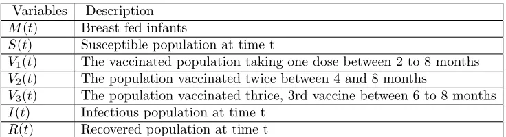
M(t) Breast fed infants
S(t) Susceptible population at time t
V1(t) The vaccinated population taking one dose between 2 to 8 months V2(t) The population vaccinated twice between 4 and 8 months
V3(t) The population vaccinated thrice, 3rd vaccine between 6 to 8 months I(t) Infectious population at time t
R(t) Recovered population at time t
We consider both fed and non-breast babies. Children are breast-fed between 0−6 months. The proportion of infants that is breast-fed is denoted by q while the birth rate is given by b. The non-breast fed fraction enters the susceptible class S(t) at a rate b(1−q). Maternal antibodies wane out at ρrate and babies from the breast-feeding class enter into susceptible class S(t).
Let the probability of becoming infected per contact with an infectious baby be denoted by β. The mass infection rate is denoted by βSI. The daily rate of first dose vaccination between 2 to 8 months is ad-ministered at a rate φ. Let τ be the daily rate at which children from
daily rate at which individuals from V2 are vaccinated for the third
time between 6 to 8 months.
Children in the different vaccination groups can come into contact with children in infected class, I(t), but the risk between these groups is reduced at different rates,η1 as the reduction in risk in case of first dose
of vaccination 0≤ η1 ≤ 1 in V1, η2 as the reduction in risk for second
dose of vaccination 0≤ η2 ≤1 in V2 and lastly, η3 as the reduction in
risk in case third dose of vaccination 0≤η3 ≤1 in V3. Since the more
times a baby is re-vaccinated the more resistant it becomes, we take
η3 ≥η2 ≥η1.
Again individuals from I(t) can recover naturally at a rate θ. The natural death rate from all the seven classes is denoted by µ. In our model, we assume that primary vaccination is available but at very low levels. Hence we consider both vaccination and treatment campaigns as our control strategies. Vaccination campaigns are considered such that more children are being vaccinated and the infected ones are being treated from the disease. We introduce vaccination as control such that the number of susceptible children increase and few become exposed to disease.
We consideru1 as the fraction of susceptibles being vaccinated per unit
time for first dose,u2 as fraction of being vaccinated for the second dose
fromV1,u3 is the fraction of babies vaccinated for the third dose from V2. We assume that every child gets the first dose of vaccination. We
further assume that the vaccine is very effective such that all vaccinated children who complete the three doses become immune and they join the recovered class R. We again bound our controls with 0≤ui ≤0.9,
for i= 1,2,3 since the entire susceptible population is not vaccinated. Children in the infected class are treated at a rate u4 who thereafter
join the recovery class with 0≤u4 ≤1 . In case of no controls, all the
control parameters are set to zero, that is, u1 =u2 =u3 =u4 = 0.
Figure 1.1. The flow chart describing our model with and without controls
The parameters are summarized in Table 2.
Table 2. parameters of the Model Parameters Description
b Birth rate
µ Death rate
q Proportion of breast feeding infants
ρ Rate of departure from breast feeding into susceptible class
β Probability of becoming infected per contact with an infectious individuals
φ The daily rate of first dose vaccination
τ The daily rate of second dose of vaccination
κ The daily rate of third dose of vaccination
η1 Reduction in risk from first vaccine (0≤η1≤1) fromV1 toI η2 Reduction in risk from second vaccine (0≤η2≤1) fromV2 toI η3 Reduction in risk from third vaccine (0≤η3≤1) fromV3to I
θ Natural recovery rate
systems.
(1.1)
dM
dt =bq−ρM−µM
dS
dt =ρM + (1−q)b−φS −βSI−µS −u1S
dV1
dt =φS−η1βV1I−τ V1−µV1−u2V1
dV2
dt =τ V1−η2βV2I−u3V2 −κV2 −µV2
dV3
dt =κV2−η3βV3I−µV3
dI
dt =βSI+ (η1V1+η2V2+η3V3)βI−(θ+µ)I−u4I
dR
dt =θI +u4I−µR+u1S+u2V1+u3V2
with intial conditions
M(0) = M0, S(0) = S0, V1(0) = V10, V2(0) = V20, V3(0) = V30, I(0) =I0, R(0) =R0.
1.2. Optimal Control Analysis. Under this Section, we investigate the optimal control efforts needed to control rotavirus disease. Controls are represented as functions of time and assigned reasonable upper and lower bounds. Vaccination with three booster doses is implemented at rate u1(t), u2(t), u3(t) for one dose, two and three doses and u4 is the
(1.2) J(u1, u2, u3, u4) =
min
(u1, u2, u3, u4) Z T
0
{I +B0(u1S+u21) +B1(u2V1+u22) +B2(u3V2+u23)
+B3(u4I+u24)}dt
whereB0, B1, B2, B3 are balancing coefficients or weight constants
trans-forming the integral into dollars expended over a finite time period ofT
days. We consider an integrand convex on the set of control parameters to indicate non-linear costs potentially arising in case of high treatment or vaccination levels. Furthermore we assume unlimited control mea-sures and the set of optimal controls (u∗1(t), u∗2(t), u∗3(t), u∗4(t))∈Ω such that
(1.3) J(u∗1, u2∗, u∗3, u∗4,) = min
Ω J(u1(t), u2(t), u3(t), u4(t))
is Lebesgue measurable and is defined as
(1.4) Ω ={(u1(t), u2(t), u3(t), u4(t))|0≤u1(t)≤u1max ≤0.9,
0≤u2(t)≤u2
max ≤0.9,0≤u3(t)≤u3max ≤0.9,0≤u4(t)≤u4max
≤1, t∈[0, T]}
Since our goal is to characterize an optimal control (u∗1, u∗2, u∗3, u∗4)∈Ω which minimizes the cost of vaccination and the cost of the treatment over the specified time interval as well as minimizes the number of infectives in a unlimited vaccination scenario. The problem is stated as follows: we have to characterize (u∗1, u∗2, u∗3, u∗4)∈Ω so that it satisfies
(1.5) J(u∗
1, u
∗
2, u
∗
3, u
∗
4) =
min
(u1, u2, u3, u4) Z T
0
{I +B0(u1S+u21) +B1(u2V1+u22) +B2(u3V2+u23)
+B3(u4I+u24)}dt
where Ω is defined in (1.4) subject to system (1.1).
Pontryagin’s maximum principle, introduces adjoint functions that al-low us to attach our state system i.e. M, S, V1, V2, V3, I, R differential
system satisfies the Lipschitz property with respect to the state vari-ables (Fleming and Rishel, 1975; Lenhart and Workman, 2007). The necessary conditions that optimal solutions must satisfy are derived using Pontryagin’s maximum principle.
This principle is used to obtain the differential equations for the adjoint variables, corresponding boundary conditions and the characterization of an optimal control set (u∗1, u∗2, u∗3, u∗4). This characterization gives a representation of an optimal control in terms of state and adjoint functions. Also this principle converts the problem of minimizing the objective functional subject to the state system into minimizing the Hamiltonian with respect to the controls (bounded measurable func-tions) at each time t.
According to (1.1) and (1.2) the Hamiltonian for our optimal control problem is:
H =I+B0(u1S+u21) +B1(u2V1+u22) +B2(u3V2+u32) +B3(u4I+u24)+
λM(t)(bq−ρM(t)−µM(t))+
λS(t)(ρM + (1−q)b−φS−βSI−µS −u1S)+
λV1(t)(φS−η1βV1I−τ V1−µV1−u2V1)+
λV2(t)(τ V1−η2βV2I−u3V2 −κV2 −µV2)+
λV3(t)(κV2−η3βV3I−µV3)+
λI(t)(βSI+ (η1V1+η2V2+η3V3)βI−(θ+µ)I−u4I)+
λR(t)(θI +u4I−µR+u1S+u2V1+u3V2).
(1.6)
where λM, λS, λV1, λV2, λV3, λI, λR are the adjoint functions associated
with their respective states. Note that, in H, each adjoint function multiplies the right-hand side of the differential equation of its corre-sponding state function. The first term inH comes from the integrand of the objective functional.
Given an optimal control set (u∗
1, u
∗
2, u
∗
3, u
∗
4) and corresponding states
(M∗, S∗, V∗
1 , V
∗
2 , V
∗
3 , I
∗, R∗), there exist adjoint functions
λM, λS, λV1, λV2, λV3, λI, λR satisfying
dλM
dt =−
∂H
∂M,
dλS
dt =−
∂H
∂S,
dλV1
dt =−
∂H
∂V1
, dλV2
dt =−
∂H
∂V2
, dλV3
dt =
−∂H
∂V3
dλI
dt =−
∂H
∂I ,
dλR
dt =−
∂H ∂R
dλX1
dt =−
∂H
∂X1
, dλX2
dt =−
∂H
∂X2
, dλX3
dt =
−∂H
∂X3
.
That is
dλM
dt =λM(ρ+µ)−λSρ
dλS
dt =λS(φ+βI(t) +µ+u1(t))−λV1φ−λIβI(t)−B0u1(t)−λRu1(t)
dλV
1
dt =λV1(η1βI(t) +τ+µ+u2(t))−λV2τ −λIη1βI(t)−B1u2(t)−λRu2
dλV
2
dt =λV2(η2βI(t) +κ+µ+u3(t))−λV3κ−λIη2βI(t)−B2u3(t)−λRu3
dλV
3
dt =λV3(η3βI(t) +µ)−λIη3βI(t)
dλI
dt =λSβS(t) +λV1η1βV1(t) +λV2η2βV2(t) +λV3η3βV3(t)−1−
λI((S(t) +η1V1(t) +η2V2(t) +η3V3(t))β−θ−u4−µ)−λR(θ+u4)
−B3u4
dλR
dt =λRµ
with the transversality conditions
(1.7)
λM(T) = 0, λS(T) = 0, λV
1(T) = 0, λV2(T) = 0, λV3(T) = 0, λI(T) = 0, λR(T) = 0
The transversality conditions i.e. the final time boundary conditions for the adjoint variables λM, λS, λV1, λV2, λV3, λI, λR are zero since there is
no dependence on the states at the final time in the objective functional.
The Hamiltonian is minimized with respect to the control (at the optimal control set) thus we differentiateHwith respect tou1, u2, u3, u4
follows:
∂H
∂u1
=B0(S+ 2u1)−λSS+λRS = 0
∂H
∂u2
=B1(V1 + 2u2)−λV
1V1 +λRV1 = 0
∂H
∂u3
=B2(V2 + 2u3)−λV
2V2 +λRV2 = 0
∂H
∂u4
=B3(I+ 2u4)−λII+λRI = 0 (1.8)
Solving for u1 = ˆu1, u2 = ˆu2, u3 = ˆu3, u4 = ˆu4 from the above set of equations, the optimality conditions are obtained as follows:
ˆ
u1 =
(λS −λR −B0)S
2B0
ˆ
u2 =
(λV1 −λR −B1)V1
2B1
ˆ
u3 = (λV2 −λR −B2)V2
2B2
ˆ
u4 =
(λI −λR −B3)I
2B3
(1.9)
Using the standard argument for control bounds, we arrive at the fol-lowing expression for the optimal control function:
u∗1(t) =min{max{0,uˆ1(t)}, u1
max}
u∗
2(t) =min{max{0,uˆ2(t)}, u2max}
u∗3(t) =min{max{0,uˆ3(t)}, u3max}
u∗4(t) =min{max{0,uˆ4(t)}, u4max}
(1.10)
dM
dt =bq−ρM−µM,
dS
dt =ρM+ (1−q)b−φS−βSI−µS−min{max{0,uˆ1(t)}, u1max}S,
dV1
dt =φS−η1βV1I−τ V1−µV1−min{max{0,uˆ2(t)}, u2max}V1,
dV2
dt =τ V1−η2βV2I−min{max{0,uˆ3(t)}, u3max}V2−κV2−µV2
dV3
dt =κV2−η3βV3I−µV3
dI
dt =βSI+ (η1V1+η2V2+η3V3)βI−(θ+µ)I−min{max{0,uˆ4(t)}, u4max}I,
dR
dt =θI+min{max{0,uˆ4(t)}, u4max}I−µR+min{max{0,uˆ1(t)}, u1max}S+
min{max{0,uˆ2(t)}, u2
max}V1+min{max{0,uˆ3(t)}, u3max}V2
(1.11)
dλM
dt =λM(ρ+µ)−λSρ
dλS
dt =λS(φ+βI(t) +µ+min{max{0,uˆ1(t)}, u1max})−λV1φ−λIβI(t)−
B0min{max{0,uˆ1(t)}, u1
max} −λRmin{max{0,uˆ1(t)}, u1max}
dλV1
dt =λV1(η1βI(t) +τ+µ+min{max{0,uˆ2(t)}, u2max})−λV2τ−
λIη1βI(t)−B1min{max{0,uˆ2(t)}, u2
max} −λRmin{max{0,uˆ2(t)}, u2max}
dλV
2
dt =λV2(η2βI(t) +κ+µ+min{max{0,uˆ3(t)}, u3max})−λV3κ−
λIη2βI(t)−B2min{max{0,uˆ3(t)}, u3
max} −λRmin{max{0,uˆ3(t)}, u3max}
dλV
3
dt =λV3(η3βI(t) +µ)−λIη3βI(t)
dλI
dt =λSβS(t) +λV1η1βV1(t) +λV2η2βV2(t) +λV3η3βV3(t)−1−
λI((S(t) +η1V1(t) +η2V2(t) +η3V3(t))β−θ−min{max{0,uˆ4(t)}, u4
λR(θ+min{max{0,uˆ4(t)}, u4
max})−B3min{max{0,uˆ4(t)}, u4max}
dλR
dt =λRµ
with initial conditions
M(0) = M0, S(0) = S0, V1(0) = V10, V2(0) = V20, V3(0) = V30, I(0) =I0, R(0) =R0
and λM(T) = 0, λS(T) = 0, λV
1(T) = 0, λV2(T) = 0, λV3(T) =
0, λI(T) = 0, λR(T) = 0.
Now, the state system of differential equations and the adjoint sys-tem of differential equations together with the control characterization above form the optimality system to be solved numerically. Since the state equations have initial conditions and the adjoint equations have final time conditions, we cannot solve the optimality system directly by only sweeping forward in time. Thus an iterative algorithm “ forward-backward sweep method ” is used. An initial estimate for the control is made. The state system is then solved forward in time from the dynamics using RK4 method. Resulting state values are placed in the right hand side of the adjoint differential equations. Then the adjoint system with given final conditions is solved backward in time, again employing RK4. Both state and adjoint values are used to update the control using characterization and then the process is repeated. This iterative process terminates when current state, adjoint and control values converge sufficiently.
2. Numerical Analysis of the Model
In this Section, we study the optimal control model (1.1) numeri-cally. We solve the model using the forward backward sweep method (Lenhart and Workman, 2007). Using the iterative method, we solve the optimality system derived in (1.11). We examine the model with three doses of vaccination controls, u1, u2, u3 and treatment u4 on
the spread of rotavirus. In our numerical analysis, we investigate and compare numerical results with different scenarios, and these include:
(i) When treatment is optimized and vaccination is set to zero, that is,u1 =u2 =u3 = 0
(ii) When controlsu1,u2,u3, that is, vaccination is optimized while
(iii) When both controls are optimized, that is, when both treatment and vaccination are optimized.
(iv) Effect of no control, with treatment only, with vaccination only, and both controls on the infected class.
We further assume the weight factors for vaccination is the same for all doses and treatment is slightly lower. The cost factors associated with treatment include, oral rehydration drugs, medical examinations and hospitalization. The parameter values used in the simulation of the model are stated in Table 3a and Table 3b.
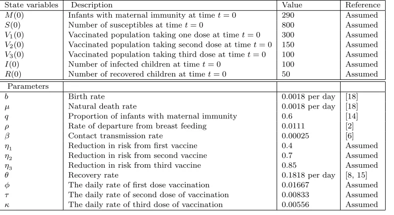
Table 3a. State variables and parameters of the Model
State variables Description Value Reference
M(0) Infants with maternal immunity at timet= 0 290 Assumed
S(0) Number of susceptibles at timet= 0 800 Assumed
V1(0) Vaccinated population taking one dose at timet= 0 300 Assumed
V2(0) Vaccinated population taking second dose at timet= 0 150 Assumed
V3(0) Vaccinated population taking third dose at timet= 0 100 Assumed
I(0) Number of infected children at timet= 0 100 Assumed
R(0) Number of recovered children at timet= 0 50 Assumed
Parameters
b Birth rate 0.0018 per day [18]
µ Natural death rate 0.0018 per day [18]
q Proportion of infants with maternal immunity 0.6 [14]
ρ Rate of departure from breast feeding 0.0111 [2]
β Contact transmission rate 0.00025 [6]
η1 Reduction in risk from first vaccine 0.4 Assumed
η2 Reduction in risk from second vaccine 0.7 Assumed
η3 Reduction in risk from third vaccine 0.85 Assumed
θ Recovery rate 0.1818 per day [8, 15]
φ The daily rate of first dose vaccination 0.01667 Assumed
τ The daily rate of second dose of vaccination 0.00833 Assumed
κ The daily rate of third dose of vaccination 0.00556 Assumed
Table 3b. Weight parameters of the Model
Parameters Description Value Reference
B0 Weight parameter for first dose 40 Assumed
B1 Weight parameter for second dose 40 Assumed
B2 Weight parameter for third dose 40 Assumed
B3 Weight parameter for treatment 5 Assumed
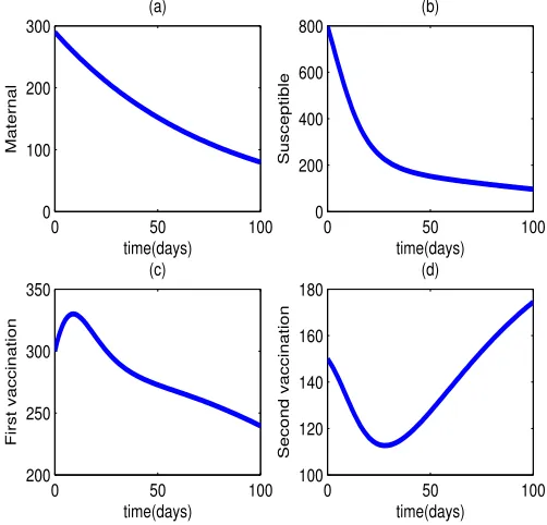
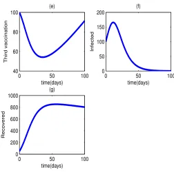
vaccination. Again from (d) children are vaccinated for the third dose and they move to class (e) as seen in Figure 2.2. Again from Figure 2.2 (f), we notice an increase in number of infected individuals who later decrease in number but after a long time, almost whent= 75 days. We lastly notice that children in the recovered class (g) take sometime to recover completely. This is due to the fact that, in absence of controls, the recovery level tends to be slow than in the presence of controls.
0 50 100
0 100 200 300
(a)
time(days)
Maternal
0 50 100
0 200 400 600 800
(b)
time(days)
Susceptible
0 50 100
200 250 300 350
(c)
time(days)
First vaccination
0 50 100
100 120 140 160 180
(d)
time(days)
Second vaccination
0 50 100 40
60 80 100
(e)
time(days)
Third vaccination
0 50 100
0 50 100 150 200
(f)
time(days)
Infected
0 50 100
0 200 400 600 800 1000
(g)
time(days)
Recovered
Figure 2.2. Profile (b) of the dynamics of rotavirus without controls
2.2. Optimal Treatment Only. Under this strategy, we optimize only treatment and all vaccination doses are put to zero, that is, u1 = u2 =u3 = 0. When treatment is optimized, we do not see any effect in
0 20 40 60 80 100 50 100 150 200 250 300 (1)
Time (in days)
Maternal
with treatment withoutcontrol
0 20 40 60 80 100
0 200 400 600 800 (2)
Time (in days)
Susceptibles
with treatment withoutcontrol
0 20 40 60 80 100
200 250 300 350 400 450 (3)
Time (in days)
First vaccination
with treatment withoutcontrol
0 20 40 60 80 100
100 150 200 250 300 (4)
Time (in days)
Second Vaccination
with treatment withoutcontrol
(a) u4profile
0 20 40 60 80 100
50 100 150 200
(5)
Time (in days)
Third vaccination
with treatment withoutcontrol
0 20 40 60 80 100
0 50 100 150 200 (6)
Time (in days)
Infected
with treatment withoutcontrol
0 20 40 60 80 100
0 200 400 600 800 1000 (7)
Time (in days)
Recovered
with treatment withoutcontrol
0 10 20 30 40 50 60 70 80 90 100 0
20 40 60 80 100 120 140 160 180
Effect of treatment on the infected class
Time (in days)
Infected
with treatment withoutcontrol
(c) Infected class with treatment only (red curve) and no treatment (blue curve)
Figure 2.3. Plots (a) and (b) shows u4 profile where
optimal control of treatment is indicated by the red curve and the blue shows no control while (c) shows the effect of treatment on the infected class (red curve) and no control (blue curve)
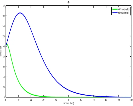
2.3. Optimal Vaccination only. Under this strategy, in Figure 2.4, we optimize vaccination, considering all the three doses, that is,u1,u2,
andu3setting the treatment control variableu4 = 0. When vaccination
0 20 40 60 80 100 50 100 150 200 250 300 (1)
Time (in days)
Maternal
with vaccination withoutcontrol
0 20 40 60 80 100
0 200 400 600 800 (2)
Time (in days)
Susceptibles
with vaccination withoutcontrol
0 20 40 60 80 100
0 100 200 300 400 (3)
Time (in days)
First vaccination
with vaccination withoutcontrol
0 20 40 60 80 100
0 50 100 150 200 (4)
Time (in days)
Second vaccination
with vaccination withoutcontrol
(a) u1, u2 and u3 profile
0 20 40 60 80 100
50 60 70 80 90 100 110 (5)
Time (in days)
Third vaccination
with vaccination withoutcontrol
0 20 40 60 80 100
0 50 100 150 200 (6)
Time (in days)
Infected
with vaccination withoutcontrol
0 20 40 60 80 100
0 500 1000 1500
(7)
Time (in days)
Recovered
with vaccination withoutcontrol
0 10 20 30 40 50 60 70 80 90 100 0
20 40 60 80 100 120 140 160 180
(6)
Time (in days)
Infected
with vaccination withoutcontrol
(c) Infected class with vaccination only (green curve) and non-vaccinated (blue curve)
Figure 2.4. A plot represents optimal vaccination only.
0 20 40 60 80 100 50 100 150 200 250 300 (1)
Time (in days)
Maternal
bothcontrols withoutcontrol
0 20 40 60 80 100
0 200 400 600 800 (2)
Time (in days)
Susceptibles
bothcontrols withoutcontrol
0 20 40 60 80 100
0 100 200 300 400 (3)
Time (in days)
One vacc
bothcontrols withoutcontrol
0 20 40 60 80 100
0 50 100 150 200 (4)
Time (in days)
Second Vacc
bothcontrols withoutcontrol
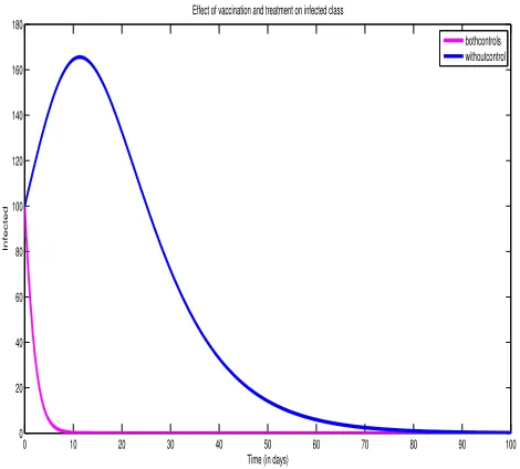
(a) u1, u2, u3 and u4 profile
0 20 40 60 80 100
50 60 70 80 90 100 110 (5)
Time (in days)
Third vacc
bothcontrols withoutcontrol
0 20 40 60 80 100
0 50 100 150 200 (6)
Time (in days)
Infected
bothcontrols withoutcontrol
0 20 40 60 80 100
0 500 1000 1500
(7)
Time (in days)
Recovered
bothcontrols withoutcontrol
(b) u1, u2, u3 and u4profile
0 10 20 30 40 50 60 70 80 90 100 0
20 40 60 80 100 120 140 160 180
Effect of vaccination and treatment on infected class
Time (in days)
Infected
bothcontrols withoutcontrol
(c) Infected class with both treatment and vaccination (pink curve) and no vaccination, no treatment (blue curve)
Figure 2.5. A plot represents optimal of both vaccina-tion and treatment.
0 10 20 30 40 50 60 70 80 90 100 0
20 40 60 80 100 120 140 160 180
Time (in days)
Infected
with treatment only without control with vaccination only both treatment and vaccination
Figure 2.6. A plot represents optimal without control (blue curve), with treatment only(red curve), with vacci-nation only(green curve), and with both treatment and treatment (pink curve)
3. Conclusion
We derived and analyzed a mathematical model for the transmission dynamics of rotavirus disease that includes vaccination administered as three booster doses and treatment as our control strategies. We performed optimal control analysis of the model by applying the con-ditions necessary for optimal control of the disease derived using the Pontryagin’s maximum principle. The numerical results show that in case of a disease outbreak we should used both control measures to reduce the infection burden within the first 10 days, otherwise, if we treat only, the infection will take 55 days to clear, if we vaccinate, the infection will take between 30 to 40 days to clear and if we do not control at all, the infection will take much longer time to clear, that is, 75 days. The later is very dangerous because if do not control the infection burden will increase hence making more children to become infected.
References
[1] Alkama, M., Elhia, M., Rachik, Z., Rachik, M., Labriji, E. (2012) Free terminal time optimal control problem of an SIR epidemic model with vaccination, International journal of science and research (IJSR), 3(5), pp. 2319-7064.
[2] Berger, R., Hadziselimovic, F., Just, M., Reigel, F. (1984) Influence of breast milk on nosocomial rotavirus infections in infants,Infections 12(4), pp. 171-174.
[3] CDC.(2009) Prevention of rotavirus gastroenteritis among infants and chil-dren: recommen- dation of the Advisory Committee on Immunization Prac-tices (ACIP),MMWR Recomm Rep,58, pp. 1-25.
[4] CDC.(2010) Report: The 9th international rotavirus sysmposium, Johan-nesburg, South Africa, held on 2-3 August 2010.
[5] CDC.(2013) Vaccine and Preventable Disease; Rotavirus Vaccine. download on Thrusday 15/08/2013 from internet, http://www.cdc.gov/vaccines/hcp/acip-recs/vacc- speci
c/rotavirus.html.
[6] Chiba, S., Nakata, S., Urasawa, T., Urasawa, S., Yokoyama, T., Morita, Y. (1986) Protective effect of naturally acquired homotypic and heterotypic rotavirus antibodies.The Lancet, 328(84), pp. 417-21.
[7] Fleming, W. H., and Rishel, R. W.(1975) Deterministic and stochastic optimal control, New York-Heidelberg-Berlin. Springer-Verlag, XIII, 22S, DM 60,60, 59(9), pp. 494-1979.
[8] Heymann, D. (2004) Gastroenteritis, acute viral: Control of communicable disease manual, 18th edition, America Public Health Association, 2004. pp. 224-227.
[9] Laarabi Hassan, Mostafa Rachik, Ouafa El Kahlaoui, El Houssine Labriji. (2013) Optimal vaccination strategies of an SIR Epidemic model of a satu-rated treatment,Universal Journal of Applied Mathematics,1(3), pp. 185-191.
[10] Lenhart, S., and Workman, J. T. (2007)
Optimal Control Applied to Biological Models.Chapman and Hall. [11] Mastretta, E., Longo, P., Laccisaglia, A., Balbo, L., Russo, R., Mazzaccara,
A., Gianino, P. (2002) Effect of Lactobacillus GG and breast-feeding in the prevention of rotavirus nosocomial infection,J. Pediatr. Gastroenterol. Nutr.35(4), pp. 527C531.
[12] Molholland, E.K. (2004) Global control of rotavirus disease.Adv Exp Med Biol,549(23), pp. 161-168.
[13] Parashar, U.D., Bresee,J.S., Gentsch,J.R., and Glass, R.I. (1998) Ro-tavirus, Emerging infectious diseases,Dis.4(4), pp. 561-570.
[15] Ruuska, T., and Vesikari, T. (1990) Rotavirus disease in Finnish children; Use of numerical scores for clinical severity of diarrhoeal episodes. Scand J. Infect Dis,22(3), pp. 259-267.
[16] Shim, E., Banks, H.T., and Castillo-Chavez, C. (2001) Seasonality of Ro-tavirus Infection with its Vaccination,J.infect. Dis, 101(1), pp. 62-92. [17] Tunde, T.Y., and Benyah, F. (2012) Optimal control of vaccination and
treatment for an SIR epidemilogical model. World journal of modelling and simulation, 8(2), pp. 194-204.
[18] VDH, (2009) Division of Health Statistics Resident Live Birth, Death , Fetal Death, and Induced Termination of Pregnancy Certificates 2009-2010, compiled by the Policy & Assessment Unit, Office of Family Health Services for Uganda. The most recent Uganda population data (2009) was used for denominators. VDH Division of Immunization.
[19] Vesikari, T., Karvonen, A., Korhonen, T. (2004) Safety and immunogenic-ity of RIX4414 live attenuated human rotavirus vaccine in adults, toddlers and previously uninfected infants,Vaccine,22(5), pp. 2836-2842.
Hellen Namawejje, Department of Mathematics, Nelson Mandela African Institution of Science and Technology, P.O.Box 447, Arusha, Tanzania
Suma Ghosh, Department of Biology, Pennsylvania State Univer-sity, University Park, State College, PA 16801, USA
Matthew Ferrari, Department of Biology, Pennsylvania State Uni-versity, University Park, State College, PA 16801, USA