Vol 2, No 11 (2013)

(1)

DOI: 10.17628/ECB.2013.2.887

CORRELATIONS OF SOLUTE PARTITIONING AND

ENTHALPIES OF SOLVATION FOR ORGANIC SOLUTES IN

IONIC LIQUIDS USING A TEMPERATURE INDEPENDENT

FREE ENERGY RELATIONSHIP

Timothy W. Stephens

a

_{, Bria Willis}

a

_{, Nishu Dabadge}

a

_{, Amy Tian}

a

_{, William E. Acree, Jr.}

a

_,

Michael H. Abraham

b

Keywords: partition coefficient,1-hexyl-3-methylimidazolium tetracyanoborate, 1-(2-methoxyethyl)-1-methylpiperidinium bis(trifluoro-methylsulfonyl)imide and 1-(2-methoxyethyl)-1-methylpyrrolidinium bis(trifluorobis(trifluoro-methylsulfonyl)imide, ionic liquids, temperature independence, linear free energy relationships, enthalpies of solvation.

Experimental data have been collected from the published literature for the gas-to-ionic liquid partition coefficients and molar enthalpies of solvation for over 60 solutes in the ionic liquids 1-hexyl-3-methylimidazolium tetracyanoborate ([MHIm]+_[B(CN)

4]–),

1-(2-methoxyethyl)-1-methylpiperidinium bis(trifluoromethylsulfonyl)imide ([MeoeMPip]+_[Tf

2N]–), and 1-(2-methoxyethyl)-1-methylpyrrolidinium

bis(trifluoromethylsulfonyl)imide ([MeoeMPyrr]+_[Tf

2N]–) over the temperature range 318.15 K to 368.15 K. The logarithm of the

gas-to-ionic liquid partition coefficient, logKL, have been correlated to a temperature independent free energy relationship utilizing known

Abraham solvation parameters. The resulting mathematical expressions describe the experimental logKL values to within a standard

deviation of 0.077 log units or less and Hsolv to within a standard deviation of 1.344 kJ mol-1 or less.

.

* Corresponding Authors Fax: 940-565-4318 E-Mail: [email protected]

[a] Department of Chemistry, 1155 Union Circle Drive #305070, University of North Texas, Denton, TX 76203-5017 (USA) [b] Department of Chemistry, University College London, 20

Gordon Street, London, WC1H OAJ (UK)

Introduction

For over twenty years, room-temperature ionic liquids (RTILs) have been used in an ever growing area of study with regards to chemical separations. One of the most prominent features of ionic liquids is the ability to fine-tune and target specific solubilizing effects based on the choice of cation or anion, or even the side chains on the cation. The RTILs 1-(2-methoxyethyl)-1-methylpiperidinium bis(trifluoromethylsulfonyl)imide ([MeoeMPip]+_[Tf

2N]–), and 1-(2-methoxyethyl)-1-methylpyrrolidinium bis(tri-fluoromethylsulfonyl)imide ([MeoeMPyrr]+_[Tf

2N]–), specifically the 2-methoxyethyl side chain, have both been shown to be particularly good at separations involving polar/non-polar azeotropic mixtures,1,2_{while the RTIL} 1-hexyl-3-methylimidazolium tetracyanoborate ([MHIm]+ [B(CN)4]–) has been shown to be very selective for aromatic and aliphatic hydrocarbons.3_{RTILs that contain the anion} [Tf2N]– have been shown to be completely immiscible with water while RTILs containing the cation [MHIm]+_have been shown to be partly soluble in water. These solubilizing characteristics allow for RTILs of this type of be used in liquid-liquid extractions between the RTIL and aqueous solution.

To date, the Abraham Solvation Parameter Model has been used to predict various solvation processes in a variety of types of solvent systems, including: the partitioning of solutes in polar organic solvents,4-9_{the partitioning of} solutes in non-polar organic solvents,10-12_{the partitioning}

within micelles,13,14_{solute partitioning within important} biological systems,15-17_{toxicity in aquatic organisms,}18-21 solute partitioning in RTILs,22-27_{and solute partitioning in} binary solvent systems.28_{The Abraham Model can be} written to predict the logarithm of the gas-to-solvent partition coefficient (logKL) and the logarithm of the water-to-solvent partition coefficient logP, as shown in Eqns. 1 and 2 respectively. The Abraham Model has also been applied in the prediction of enthalpies of solvation,29-34_as shown in Eqn. 3.

log KL = cK + eK E + sK S + aK A + bK B + lK L (1)

log P = cP + eP E + sP S + aP A + bP B + vP V (2)

ΔHsolv = cH,solv + eH,solv E + sH,solv S + aH,solv A + bH,solv B + lH,solv L (3)

(2)

measure of the solvent system’s interactions with the solute’s - and non-bonding electrons, s is a measure of the solvent system’s combined polarizability and dipolarity, a is a measure of the solvent system’s hydrogen-bond basicity and is complimentary to the solute’s hydrogen-bond acidity,

b is a measure of the solvent system’s hydrogen-bond acidity and is complimentary to the solute’s hydrogen-bond basicity, and l and v are measures of general dispersion forces necessary to create a cavity in the solvent system for solubilizing the solute. When the solvent coefficients are combined with their complimentary descriptors, the resulting product can be used to characterize that particular solute-solvent interaction. For the partitioning between two condensed phases, the coefficient values can be used to indicate the differences between the two phases of that particular property.

Sprunger, et al.41-43_{have expanded the Abraham Model} so that the gas-to-RTIL partition coefficient can be predicted based on ion-specific coefficients for individual cations and anions, as shown in Eqn. 4. Utilizing the ion-specific coefficients, RTILs can be synthesized that take advantage of specific properties that may be attractive for specific separations.

log KL = (cK,cation + cK,anion) + (eK,cation + eK,anion) E + (sK,cation + sK,anion) S + (aK,cation + aK,anion) A + (bK,cation + bK,anion) B + (lK,cation + lK,anion) L (4) Mintz, et al.44_{and Sprunger, et al.}45_{describe a basis for} incorporating temperature dependent terms into the Abraham Model that comes from the Gibbs’ Free Energy Relationship, Eqn. 5, and the relation between Gsolv and KL, Eqn. 6, where R is the universal gas constant in units of J mol-1_K-1_,_T_{is the temperature of the system in Kelvin, and} KL is the gas-to-solvent partition coefficient.

ΔGsolv = ΔHsolv – T ΔSsolv (5) ΔGsolv = –RT ln KL (6)

Converting Eqn. 6 from base e to base 10 so that the results correspond to previous Abraham Model correlations, yields Eqn. 7.

ΔGsolv = –2.303 RT log KL (7)

Using Eqns. 1, 3, 5 and 7, the Abraham Model can be applied to the prediction of Ssolv, expressed as Eqn. 8.

ΔSsolv = cS,solv + eS,solvE + sS,solvS + aS,solvA + bS,solvB

+ lS,solvL (8)

Eqns. 3, 5, 7, and 8 can now be combined and rewritten as Eqn. 9, and simplified into Eqn. 10.

–2.303 RT log KL = cH,solv + eH,solvE + sH,solvS + aH,solvA + bH,solvB + lH,solvL – T (cS,solv + eS,solvE + sS,solvS +

aS,solvA + bS,solvB + lS,solvL ) (9)

Because of the relationship between log KL and ΔHsolv, the cH, eH, sH, aH, bH, and lH coefficients from Eqn. 10 should

yield the same coefficients as for Eqn. 3.

Data sets and computation methodology

Gas-to-solvent partition coefficients KL were found for the RTILs 1-hexyl-3-methylimidazolium tetracyanoborate ([MHIm]+_[B(CN)

4]–),3 1-(2-methoxyethyl)-1-methylpipe-ridinium bis(trifluoromethylsulfonyl)imide ([MeoeMPip]+ [Tf2N]–),2 and 1-(2-methoxyethyl)-1-methylpyrrolidinium bis(trifluoromethylsulfonyl)imide ([MeoeMPyrr]+_[Tf

2N]–)1 by performing a search of the chemical literature. All of the partition coefficients were converted to logKL and tabulated with the necessary solute descriptors in a 12 column matrix. Enthalpies of solvation were calculated using the relationship given in Eqn. 11 and tabulated with the necessary solute descriptors into a 5 column matrix. A linear regression was performed on each matrix using the statistical software program SPSS 20.0. For the logKL correlation, the linear regression was forced through the origin. For the Hsolv correlation, the linear regression was not forced through the origin.

ΔHsolv = –2.303 R [d log KL/ d(1/T)] (11)

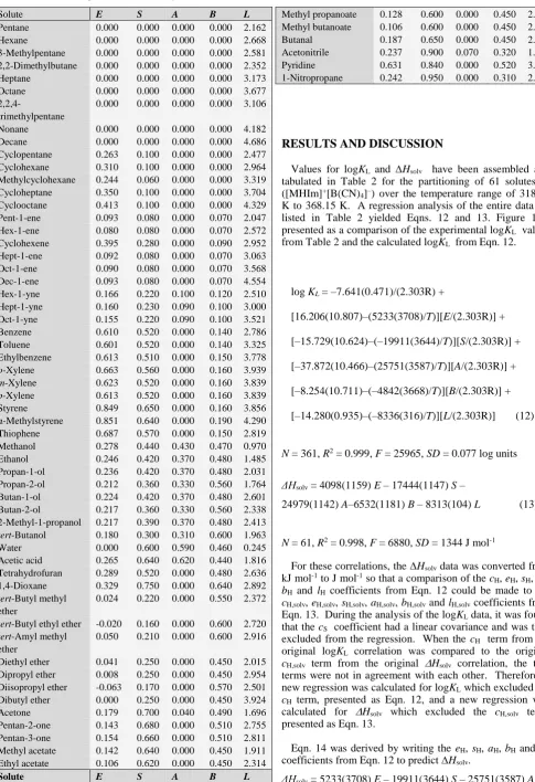
Table 1 lists all solute descriptors used for the analysis of the three RTILs. The solute descriptors used came from a database that the authors have compiled and were initially obtained using experimental data such as water-to-solvent partition coefficients, gas-to-solvent partition coefficients, solubility, and chromatographic data. Numerical values for the descriptors used in the analysis of the three ionic liquids cover the same area of predictive space, with values for each descriptor ranging from: E = –0.063 to E = 0.851, S = 0.000 to S = 0.950, A = 0.000 to A = 0.820, B = 0.000 to B = 0.640, and L = 0.260 to L = 4.686. The solutes used in each correlation show a wide range of functionality as well as non-polar and polar characteristics. For all correlations, the authors report the N (number of data points), R2_{(square of} the correlation coefficient), F (Fisher’s F-Statistic), and SD

(standard deviation).

1

H H

log

S S

2.303 2.303

H H

S S

2.303 2.303

H H ₍₁₀₎

S S

2.303 2.303

c e E

K c e

T R T R

s S a A

s a

T R T R

b B l L

b l

T R T R

    

   

  

































































(3)

DOI: 10.17628/ECB.2013.2.887

Table 1. Solute descriptors used in the analyses

Solute E S A B L

Pentane 0.000 0.000 0.000 0.000 2.162

Hexane 0.000 0.000 0.000 0.000 2.668

3-Methylpentane 0.000 0.000 0.000 0.000 2.581 2,2-Dimethylbutane 0.000 0.000 0.000 0.000 2.352

Heptane 0.000 0.000 0.000 0.000 3.173

Octane 0.000 0.000 0.000 0.000 3.677

2,2,4-trimethylpentane

0.000 0.000 0.000 0.000 3.106

Nonane 0.000 0.000 0.000 0.000 4.182

Decane 0.000 0.000 0.000 0.000 4.686

Cyclopentane 0.263 0.100 0.000 0.000 2.477 Cyclohexane 0.310 0.100 0.000 0.000 2.964 Methylcyclohexane 0.244 0.060 0.000 0.000 3.319 Cycloheptane 0.350 0.100 0.000 0.000 3.704 Cyclooctane 0.413 0.100 0.000 0.000 4.329 Pent-1-ene 0.093 0.080 0.000 0.070 2.047

Hex-1-ene 0.080 0.080 0.000 0.070 2.572

Cyclohexene 0.395 0.280 0.000 0.090 2.952 Hept-1-ene 0.092 0.080 0.000 0.070 3.063

Oct-1-ene 0.090 0.080 0.000 0.070 3.568

Dec-1-ene 0.093 0.080 0.000 0.070 4.554

Hex-1-yne 0.166 0.220 0.100 0.120 2.510

Hept-1-yne 0.160 0.230 0.090 0.100 3.000

Oct-1-yne 0.155 0.220 0.090 0.100 3.521

Benzene 0.610 0.520 0.000 0.140 2.786

Toluene 0.601 0.520 0.000 0.140 3.325

Ethylbenzene 0.613 0.510 0.000 0.150 3.778

o-Xylene 0.663 0.560 0.000 0.160 3.939

m-Xylene 0.623 0.520 0.000 0.160 3.839

p-Xylene 0.613 0.520 0.000 0.160 3.839

Styrene 0.849 0.650 0.000 0.160 3.856

α-Methylstyrene 0.851 0.640 0.000 0.190 4.290

Thiophene 0.687 0.570 0.000 0.150 2.819

Methanol 0.278 0.440 0.430 0.470 0.970

Ethanol 0.246 0.420 0.370 0.480 1.485

Propan-1-ol 0.236 0.420 0.370 0.480 2.031 Propan-2-ol 0.212 0.360 0.330 0.560 1.764 Butan-1-ol 0.224 0.420 0.370 0.480 2.601 Butan-2-ol 0.217 0.360 0.330 0.560 2.338 2-Methyl-1-propanol 0.217 0.390 0.370 0.480 2.413

tert-Butanol 0.180 0.300 0.310 0.600 1.963

Water 0.000 0.600 0.590 0.460 0.245

Acetic acid 0.265 0.640 0.620 0.440 1.816 Tetrahydrofuran 0.289 0.520 0.000 0.480 2.636 1,4-Dioxane 0.329 0.750 0.000 0.640 2.892

tert-Butyl methyl ether

0.024 0.220 0.000 0.550 2.372

tert-Butyl ethyl ether -0.020 0.160 0.000 0.600 2.720

tert-Amyl methyl ether

0.050 0.210 0.000 0.600 2.916

Diethyl ether 0.041 0.250 0.000 0.450 2.015 Dipropyl ether 0.008 0.250 0.000 0.450 2.954 Diisopropyl ether -0.063 0.170 0.000 0.570 2.501 Dibutyl ether 0.000 0.250 0.000 0.450 3.924

Acetone 0.179 0.700 0.040 0.490 1.696

Pentan-2-one 0.143 0.680 0.000 0.510 2.755 Pentan-3-one 0.154 0.660 0.000 0.510 2.811 Methyl acetate 0.142 0.640 0.000 0.450 1.911 Ethyl acetate 0.106 0.620 0.000 0.450 2.314

Solute E S A B L

Methyl propanoate 0.128 0.600 0.000 0.450 2.431 Methyl butanoate 0.106 0.600 0.000 0.450 2.893

Butanal 0.187 0.650 0.000 0.450 2.270

Acetonitrile 0.237 0.900 0.070 0.320 1.739

Pyridine 0.631 0.840 0.000 0.520 3.022

1-Nitropropane 0.242 0.950 0.000 0.310 2.894

RESULTS AND DISCUSSION

Values for logKL and Hsolv have been assembled and tabulated in Table 2 for the partitioning of 61 solutes in ([MHIm]+_[B(CN)

4]–) over the temperature range of 318.15 K to 368.15 K. A regression analysis of the entire data set listed in Table 2 yielded Eqns. 12 and 13. Figure 1 is presented as a comparison of the experimental logKL values from Table 2 and the calculated logKL from Eqn. 12.

log KL = –7.641(0.471)/(2.303R) +

[16.206(10.807)–(5233(3708)/T)][E/(2.303R)] +

[–15.729(10.624)–(–19911(3644)/T)][S/(2.303R)] +

[–37.872(10.466)–(25751(3587)/T)][A/(2.303R)] +

[–8.254(10.711)–(–4842(3668)/T)][B/(2.303R)] +

[–14.280(0.935)–(–8336(316)/T)][L/(2.303R)] (12)

N = 361, R2_{= 0.999,}_F_{= 25965,}_SD_{= 0.077 log units} ΔHsolv= 4098(1159) E – 17444(1147) S –

24979(1142) A–6532(1181) B – 8313(104) L (13) (13)

N = 61, R2_{= 0.998,}_F_{= 6880,}_SD_{= 1344 J mol}-1

For these correlations, the Hsolv data was converted from kJ mol-1_{to J mol}-1_{so that a comparison of the}_c

H, eH, sH, aH, bH and lH coefficients from Eqn. 12 could be made to the cH,solv, eH,solv, sH,solv, aH,solv, bH,solv and lH,solv coefficients from Eqn. 13. During the analysis of the logKL data, it was found that the cS coefficient had a linear covariance and was thus excluded from the regression. When the cH term from the original logKL correlation was compared to the original cH,solv term from the original Hsolv correlation, the two terms were not in agreement with each other. Therefore, a new regression was calculated for logKL which excluded the cH term, presented as Eqn. 12, and a new regression was calculated for Hsolv which excluded the cH,solv term, presented as Eqn. 13.

Eqn. 14 was derived by writing the eH, sH, aH, bH and lH, coefficients from Eqn. 12 to predict Hsolv.

(4)

4842(3688) B – 8336(316) L (14)

SD = 1424 J mol-1_,_AAE_{= 1064 J mol}-1_,_AE_{= 192 J mol}-1 Reported are the SD, AAE (absolute average error), and

AE (average error) for the prediction of Hsolv based on Eqn. 14. As shown, Eqn. 14 predictsHsolv to within a similar standard deviation as Eqn. 13. The very low AE and AAE

values show very little bias between using Eqn. 13 or Eqn. 14 to predictHsolv. Eqn. 14 also illustrates that the eH, sH, aH, bH and lH coefficients from Eqn. 12 and the eH,solv, sH,solv, aH,solv, bH,solv and lH,solv coefficients from Eqn. 13 are individually within the statistical error of their respective counterparts.

Figure 1. Graph of experimental logarithm of gas-to-[MHIm]+_[B(CN)

4]- partition coefficient (logKL) versus calculated

logKL based on Eq. 12.

As an informational note one could develop Abraham model correlations for each individual temperature. As noted by Mintz et al.44_{and Sprunger et al.}45_{offers over such} temperature-specifc correlations is that one can develop correlations for more partitioning process and for more ionic liquid solvents. For example, lets assume that one was able to find log KL data 20 solutes in ([MHIm]+[B(CN)4]–) at 298 K, log KL data for a different set of 20 solutes in

([MHIm]+_[B(CN)

4]–) at 318.15 K, and log KL data for a third

set of 20 different solutes in ([MHIm]+_[B(CN)

4]–) at 368 K. There would be insufficient experimental data to develop a meaningful Abraham model correlation at any of the three temperatures mentioned. However, by pooling the 60 log

KL values for ([MHIm]+ [B(CN)4]–) into a single dataset, one could develop a predictive correlation based on Eqn. 10. Such predictions would not be possible with Eqn. 1 which requires that all of the experimental data be at the same temperature.

To determine the predictability of Eqn. 12, the data in Table 2 was analyzed using a training set and test analysis. In this method of analysis, the complete data set is randomly split in half and divided into a training set and a test set. In the event that the complete data set has an odd number of data points, the extra data point is included in the training set. A linear regression is then performed on the training set and a new training correlation is calculated. This training

correlation is then used to predict the values in the test set, and the SD, AAE, and AE are reported. Eqn. 15 is the resultant correlation from randomly splitting half of the logKL data reported in Table 2. Using Eqn. 15 to predict the values in the test set yielded a SD = 0.083 log units, AAE = 0.055, and AE = -0.004. The very small difference in the coefficient values calculated between the training set and parent set show that the training set compounds and temperatures are representative of the parent compounds and temperatures. The low AE value shows very little bias between using Eqns. 12 and 15.

log KL = –7.699(0.653)/(2,303 R) +

[15.446(14.979) – (4914(5133)/T)] [E/(2.303 R)] +

[–14.226(15.704) – (–19294(5388)/T)][S/(2.303 R)] +

[–58.028(17.935) – (–33067(6232)/T)] [A/(2.303 R)] +

[–9.661(15.007) – (–5405(5189)/T)] [B/(2.303 R)] +

[–14.012(1.297) – (–8245(445)/T)] [L/(2.303 R)] (15)

N = 181, R2_{= 0.999,}_F_{= 13690,}_SD_{= 0.074 log units} Values for logKL and Hsolv have been assembled and tabulated in Table 3 for the partitioning of 61 solutes in ([MeoeMPip]+_[Tf

2N]–) over the temperature range of 318.15 K to 368.15 K. A regression analysis of the entire data set listed in Table 3 yielded Eqns. 16 and 17. Figure 2 is presented as a comparison of the experimental logKL values from Table 3 and the calculated logKL from Eqn. 16.

log KL = –10.878(0.387)/(2.303 R) +

[0.536(6.437) – (–14440(2202)/T)][S/(2.303 R)] +

[–29.947(9.729) – (–23020(3325)/T)] [A/(2.303 R)] +

[–17.927(7.920) – (–7332(2707)/T)] [B/(2.303 R)] +

[–12.721(0.706) – (–7802(239)/T)] [L/(2.303 R)] (16)

N = 365, R2_{= 0.999,}_F_{= 31686,}_SD_{= 0.069 log units}

ΔHsolv = –14486(805) S – 22955(1223) A –

7248(991) B –7791(88) L (17)

N = 61, R2_{= 0.998,}_F_{= 7868,}_SD_{= 1335 J/mol}

H, eH, sH, aH, bH and lH coefficients from Eqn. 16 could be made to the cH,solv, eH,solv, sH,solv, aH,solv, bH,solv and lH,solv coefficients from Eqn. 17. Coincidentally, during the analysis of the logKL data for ([MeoeMPip]+_[Tf

(5)

DOI: 10.17628/ECB.2013.2.887

the original logKL correlation was compared to the original cH,solv term from the original Hsolv correlation, the two terms were also not in agreement with each other, as occurred for ([MHIm]+_[B(CN)

4]–). Further analysis of the correlation for logKL showed that the eS and eH terms were very small, 9.267(8.538) and 1986(2921) respectively. These terms were subsequently set equal to zero and the regression was performed once again. Eqn. 16 is the resultant correlation obtained by removing the cH, eS and eH terms and Eqn. 17 is the resultant correlation obtained when the cH,solv and eH,solv terms are removed.

Eqn. 18 was derived by writing the sH, aH, bH and lH, coefficients from Eqn. 16 to predict Hsolv.

ΔHsolv = –14440(2202) S – 23020(3325) A – 7332(2707) B – 7802(239) L (18)

SD = 1335 J mol-1_,_AAE_{= 1011 J mol}-1_,_AE_{= -93 J mol}-1_. Reported are the SD, AAE, and AE for the prediction of

Hsolv based on Eqn. 18. As shown, Eqn. 18 predicts Hsolv to within the same standard deviation as Eqn. 17. The very low AE and AAE values show very little bias between using Eqn. 17 or Eqn. 18 to predictHsolv. Eqn. 18 also illustrates that the sH, aH, bH and lH coefficients from Eqn. 16 and the sH,solv, aH,solv, bH,solv and lH,solv coefficients from Eqn. 17 are individually within the statistical error of their respective counterparts.

Figure 2. Graph of experimental logarithm of gas-to-([MeoeMPip]+_[Tf

2N]–) partition coefficient (logKL) versus

calculated logKL based on Eqn. 16.

To determine the predictability of Eqn. 16, the data in Table 3 was also analyzed using a training set and test analysis. Eqn. 19 is the resultant correlation from randomly splitting half of the logKL data reported in Table 3. Using Eqn. 19 to predict the values in the test set yielded a SD = 0.071 log units, AAE = 0.053, and AE = 0.002.

The very small difference in the coefficient values calculated between the training set and parent set show that the training set compounds and temperatures are representative of the parent compounds and temperatures. The low AE value shows very little bias between using Eqns. 16 and 19.

log KL = –10.992(0.562)/(2.303 R) +

[5.061(9.173) – (–12834(3131)/T)][S/(2.303 R)] +

[–16.206(14.399) – (–18341(4871)/T)] [A/(2.303 R)] +

[–27.181(12.155) – (–10547(4150)/T)] [B/(2.303 R)] +

[–12.610(0.926) – (–7777(307)/T)] [L/(2.303 R)]

(19)

N = 183, R2_{= 0.999,}_F_{= 17102,}_SD_{= 0.068 log units} It should be noted that Marciniak and Wlazło2_also corelated the log KL data for ([MeoeMPip]+[Tf2N]–) in terms of the Abraham model. The authors developed temperature-specific correlations in the form of Eqn. 1 for each of the six temperatures studied. A total of 36 curve-fit equation coefficients were needed to describe the 365 experimental data points to an average standard deviation of SD = 0.059 log units. Our method, Eqn. 16, has only nine curve-fit equation coefficients and describes the 365 log KL values to

within SD = 0.069 log units. Very little loss in predictive ability resulted from our method of combining all 365 experimental values into a single regression analysis.

Values for logKL and Hsolv have been assembled and tabulated in Table 4 for the partitioning of 61 solutes in ([MeoeMPyrr]+_[Tf

2N]–) over the temperature range of 318.15 K to 368.15 K. A regression analysis of the entire data set listed in Table 4 yielded Eqns. 20 and 21. Figure 3 is presented as a comparison of the experimental logKL values from Table 4 and the calculated logKL from Eqn. 20.

log KL = –10.033(0.375)/(2.303 R) +

[10.075(8.499) – (2557(2905)/T)] [E/(2.303 R)] +

[–7.117(8.475) – (–16471(2897)/T)][S/(2.303 R)] +

[–33.881(9.165) – (–24144(3132)/T)] [A/(2.303 R)] +

[–12.474(8.752) – (–6027(2992)/T)] [B/(2.303 R)] +

[–13.508(0.763) – (–7875(258)/T)] [L/(2.303 R)] (20)

N = 366, R2_{= 0.999,}_F_{= 30869,}_SD_{= 0.064 log units}

ΔHsolv = –2534(1090) E – 16481(1086) S –

24066(1175)A– 5998(1123) B – 7856(97) L (21)

N = 61, R2_{= 0.998, F = 6976, SD = 1260 J/mol}

H, eH, sH, aH, bH and lH coefficients from Eqn. 20 could be made to the cH,solv, eH,solv, sH,solv, aH,solv, bH,solv and lH,solv coefficients from Eqn. 21. Coincidentally, during the analysis of the logKL data for ([MeoeMPyrr]+_[Tf

(6)

thus excluded from the regression. When the cH term from the original logKL correlation was compared to the original cH,solv term from the original Hsolv correlation, the two terms were also not in agreement with each other, as occurred for ([MHIm]+_[B(CN)

4]–) and ([MeoeMPip]+ [Tf2N]–). Once again, Eqn. 20 is the resultant correlation obtained by removing the cH term and Eqn. 21 is the resultant correlation obtained when the cH,solv term is removed.

Eqn. 22 was derived by writing the eH, sH, aH, bH, and lH coefficients from Eqn. 20 to predict Hsolv.

ΔHsolv = 2557(2905) E – 16471(2897) S –

24144(3132) A – 6027(2992) B – 7875(258) L (22)

SD = 1263 J mol-1_,_AAE_{= 1005 J mol}-1_,_AE_{= -7 J mol}-1 Reported are the SD, AAE, and AE for the prediction of

Hsolv based on Eqn. 22. As shown, Eqn. 22 predicts Hsolv to within a similar standard deviation as Eqn. 21. The very low AE and AAE values show very little bias between using Eqn. 21 or Eqn. 22 to predictHsolv. Eqn. 22 also illustrates that the eH, sH, aH, bH and lH coefficients from Eqn. 20 and the cH,solv, eH,solv, sH,solv, aH,solv, bH,solv and lH,solv coefficients from Eqn. 21 are individually within the statistical error of their respective counterparts.

Table 2. Logarithm of gas-to-([MHIm]+_[B(CN)

4]–) partition coefficients at various temperatures and enthalpies of solvation (in kJ mol-1)a

Solute logKL Hsolv

kJ mol-1

Temperature, K 318.15 328.15 338.15 348.15 358.15 368.15

Pentane 0.917 0.820 0.732 0.645 0.569 0.496 -18.887

Hexane 1.246 1.130 1.021 0.919 0.827 0.736 -22.814

3-Methylpentane 1.215 1.100 0.997 0.898 0.808 0.720 -22.131

2,2-Dimethylbutane 1.025 0.923 0.830 0.739 0.658 0.580 -19.965

Heptane 1.567 1.431 1.305 1.188 1.079 0.977 -26.423

Octane 1.884 1.728 1.583 1.446 1.322 1.204 -30.448

2,2,4-Trimethylpentane 1.491 1.362 1.241 1.124 1.021 0.922 -25.547

Nonane 2.196 2.021 1.857 1.703 1.565 1.431 -34.262

Decane 2.508 2.310 2.130 1.959 1.805 1.658 -38.033

Cyclopentane 1.365 1.255 1.155 1.057 0.970 0.885 -21.531

Cyclohexane 1.679 1.555 1.439 1.332 1.228 1.134 -24.481

Methylcyclohexane 1.840 1.704 1.581 1.459 1.350 1.246 -26.650

Cycloheptane 2.179 2.033 1.892 1.760 1.640 1.526 -29.312

Cyclooctane 2.615 2.442 2.283 2.134 1.994 1.863 -33.670

Hex-1-ene 1.459 1.336 1.220 1.111 1.009 0.915 -24.433

Cyclohexene 1.985 1.846 1.720 1.593 1.484 1.378 -27.185

Hept-1-ene 1.779 1.634 1.501 1.375 1.260 1.149 -28.194

Oct-1-ene 2.093 1.930 1.777 1.633 1.504 1.380 -31.974

Dec-1-ene 2.714 2.508 2.324 2.146 1.985 1.832 -39.487

Hex-1-yne 2.029 1.879 1.740 1.606 1.486 1.371 -29.510

Hept-1-yne 2.352 2.182 2.025 1.873 1.736 1.607 -33.403

Oct-1-yne 2.666 2.476 2.299 2.130 1.980 1.836 -37.206

Benzene 2.629 2.471 2.320 2.182 2.053 1.931 -31.295

Toluene 2.982 2.801 2.629 2.473 2.326 2.188 -35.599

Ethylbenzene 3.252 3.053 2.866 2.695 2.534 2.384 -38.901

o-Xylene 3.464 3.254 3.058 2.879 2.710 2.553 -40.820

m-Xylene 3.316 3.110 2.919 2.744 2.579 2.425 -39.887

p-Xylene 3.310 3.103 2.915 2.737 2.574 2.420 -39.850

Styrene 3.441 3.239 3.052 2.878 2.715 -41.945

α-Methylstyrene 3.614 3.395 3.195 3.007 2.831 -45.191

Methanol 2.400 2.250 2.111 1.984 1.865 1.757 -28.807

Ethanol 2.582 2.418 2.267 2.127 1.994 1.874 -31.737

Propan-1-ol 2.925 2.739 2.569 2.408 2.260 2.127 -35.771

Propan-2-ol 2.625 2.452 2.292 2.143 2.009 1.884 -33.194

Butan-1-ol 3.279 3.072 2.880 2.703 2.542 2.391 -39.749

Butan-2-ol 2.952 2.759 2.582 2.417 2.267 2.127 -36.920

2-Methyl-1-propanol 3.087 2.891 2.708 2.539 2.384 2.238 -38.043

tert-Butanol 2.631 2.452 2.290 2.137 1.993 1.864 -34.386

Water 2.668 2.505 2.356 2.217 2.090 1.964 -31.458

Acetic acid 3.540 3.340 3.153 2.979 2.816 -41.860

(7)

DOI: 10.17628/ECB.2013.2.887

Temperature, K 318.15

_{kJ mol}

-1 _338.15 _348.15 _358.15 _368.15 _{kJ mol}-1

Thiophene 2.759 2.593 2.441 2.301 2.167 2.045 -31.953

Tetrahydrofuran 2.626 2.465 2.318 2.179 2.053 1.935 -30.959

1,4-Dioxane 3.295 3.101 2.921 2.754 2.599 2.452 -37.775

tert-Butyl methyl ether 1.914 1.768 1.634 1.507 1.391 1.281 -28.346

tert-Butyl ethyl ether 1.839 1.689 1.553 1.422 1.301 1.188 -29.186

tert-Amyl methyl ether 2.248 2.083 1.933 1.790 1.660 1.535 -31.894

Diethyl ether 1.623 1.496 1.378 1.265 1.161 1.064 -25.063

Dipropyl ether 2.076 1.920 1.775 1.636 1.511 1.391 -30.694

Diisopropyl ether 1.759 1.612 1.473 1.342 1.225 1.114 -28.922

Dibutyl ether 2.689 2.496 2.316 2.143 1.987 1.839 -38.115

Acetone 2.621 2.468 2.326 2.196 2.072 1.958 -29.707

Pentan-2-one 3.176 2.987 2.813 2.650 2.501 2.360 -36.526

Pentan-3-one 3.182 2.993 2.816 2.652 2.502 2.360 -36.822

Methyl acetate 2.456 2.299 2.152 2.021 1.893 1.773 -30.557

Ethyl acetate 2.661 2.486 2.326 2.182 2.041 1.915 -33.372

Methyl propanoate 2.735 2.559 2.394 2.243 2.104 1.975 -34.044

Methyl butanoate 3.002 2.810 2.630 2.467 2.316 2.173 -37.080

Butanal 2.944 2.789 2.644 2.512 2.387 2.272 -30.120

Acetonitrile 3.502 3.309 3.125 2.958 2.800 2.651 -38.133

Pyridine 3.473 3.285 3.111 2.950 2.797 -39.012

1-Nitropropane 3.473 3.285 3.111 2.950 2.797 -39.012

a _{Experimental gas-to-liquid partition coefficient data taken from Domańska et al.}3

Table 3. Logarithm of gas-to-([MeoeMPip]+_[Tf

2N]–) partition coefficients at various temperatures and enthalpies of solvation

(in kJ mol-1₎a

Solute logKL Hsolv

kJ mol-1

Temperature, K 318.15 K 328.15 K 338.15 K 348.15 K 358.15 K 368.15 K

Pentane 0.751 0.653 0.565 0.486 0.413 0.344 -18.120

Hexane 1.061 0.944 0.841 0.746 0.658 0.574 -21.706

3-Methylpentane 1.041 0.926 0.824 0.732 0.648 0.566 -21.169

2,2-Dimethylbutane 0.884 0.780 0.688 0.604 0.525 0.452 -19.293

Heptane 1.365 1.230 1.111 0.999 0.899 0.798 -25.292

Octane 1.662 1.509 1.371 1.246 1.127 1.021 -28.653

Nonane 1.958 1.785 1.630 1.490 1.358 1.236 -32.259

Decane 2.248 2.057 1.888 1.730 1.583 1.444 -35.887

Cyclopentane 1.176 1.068 0.969 0.879 0.794 0.714 -20.638

Cyclohexane 1.476 1.350 1.238 1.134 1.037 0.947 -23.604

Cycloheptane 1.926 1.780 1.645 1.524 1.413 1.307 -27.621

Cyclooctane 2.326 2.161 2.009 1.870 1.742 1.621 -31.537

Pent-1-ene 0.961 0.857 0.765 0.679 0.601 0.526 -19.393

Hex-1-ene 1.274 1.155 1.041 0.943 0.846 0.758 -23.104

Cyclohexene 1.763 1.628 1.508 1.393 1.288 1.190 -25.619

Hept-1-ene 1.579 1.438 1.307 1.193 1.083 0.983 -26.638

Oct-1-ene 1.876 1.716 1.569 1.438 1.312 1.196 -30.392

Dec-1-ene 2.458 2.262 2.083 1.919 1.765 1.618 -37.540

Hex-1-yne 1.862 1.713 1.576 1.450 1.332 1.223 -28.601

Hept-1-yne 2.161 1.995 1.841 1.699 1.566 1.442 -32.200

Oct-1-yne 2.456 2.272 2.100 1.943 1.795 1.658 -35.754

Benzene 2.505 2.348 2.201 2.064 1.941 1.825 -30.493

Toluene 2.833 2.654 2.489 2.336 2.193 2.061 -34.568

Ethylbenzene 3.084 2.889 2.708 2.539 2.384 2.238 -37.904

o-Xylene 3.289 3.085 2.895 2.719 2.556 2.403 -39.667

m-Xylene 3.166 2.967 2.783 2.612 2.452 2.303 -38.658

p-Xylene 3.146 2.945 2.760 2.589 2.430 2.279 -38.806

Styrene 3.502 3.289 3.090 2.908 2.740 2.580 -41.258

α-Methylstyrene 3.457 3.244 3.050 2.866 2.693 -44.091

Thiophene 2.636 2.473 2.322 2.182 2.053 1.932 -31.538

(8)

Temperature, K 318.15 K 318.15 K 318.15 K 318.15 K 318.15 K 318.15 K

_{kJ mol}

-1

Pyridine 3.314 3.125 2.948 2.784 2.631 2.490 -36.943

Methanol 2.158 2.017 1.887 1.770 1.660 1.556 -26.906

Ethanol 2.336 2.182 2.037 1.906 1.781 1.665 -30.082

Propan-1-ol 2.640 2.465 2.303 2.158 2.017 1.889 -33.637

Propan-2-ol 2.391 2.223 2.068 1.930 1.800 1.679 -31.795

Butan-1-ol 2.970 2.773 2.592 2.428 2.274 2.134 -37.420

Butan-2-ol 2.669 2.481 2.316 2.161 2.021 1.889 -34.815

2-Methyl-propan-1-ol 2.799 2.607 2.431 2.274 2.127 1.992 -36.095

tert-Butanol 2.408 2.230 2.072 1.926 1.792 1.671 -32.935

Water 2.427 2.281 2.137 2.013 1.898 1.788 -28.590

Methyl acetate 2.288 2.134 1.993 1.862 1.742 1.630 -29.419

Ethyl acetate 2.493 2.324 2.167 2.025 1.893 1.770 -32.340

1,4-Dioxane 3.034 2.850 2.679 2.520 2.373 2.233 -35.879

tert-Butyl methyl ether 1.686 1.545 1.418 1.299 1.190 1.090 -26.666

tert-Butyl ethyl ether 1.590 1.450 1.322 1.204 1.097 0.994 -26.629

tert-Amyl methyl ether 1.986 1.831 1.688 1.556 1.435 1.320 -29.814

Diethyl ether 1.380 1.262 1.152 1.053 0.959 0.872 -22.752

Dipropyl ether 1.819 1.668 1.530 1.403 1.286 1.176 -28.761

Dibutyl ether 2.375 2.190 2.021 1.866 1.721 1.584 -35.348

Acetone 2.452 2.303 2.164 2.037 1.917 1.806 -28.926

Pentan-2-one 2.947 2.765 2.598 2.441 2.297 2.161 -35.193

Pentan-3-one 2.938 2.757 2.588 2.430 2.286 2.149 -35.338

Butanal 2.507 2.348 2.201 2.064 1.941 1.824 -30.568

Acetonitrile 2.830 2.679 2.538 2.407 2.283 2.170 -29.577

1-Nitropropane 3.478 3.280 3.097 2.927 2.769 2.621 -38.370

a _{Experimental gas-to-liquid partition coefficient data taken from Marciniak and Wlazło.}2

Table 4. Logarithm of gas-to-([MeoeMPyrr]+ _[Tf

2N]–) partition coefficients at various temperatures and enthalpies of solvation

(in kJ mol-1₎a

Solute

Temperature, K

logKL Hsolv

kJ mol-1

318.15 K 328.15 K 338.15 K 348.15 K 358.15 K 368.15 K

Pentane 0.717 0.623 0.537 0.458 0.386 0.322 -17.685

Hexane 1.029 0.919 0.817 0.719 0.633 0.551 -21.422

3-Methylpentane 1.009 0.897 0.794 0.702 0.614 0.538 -21.093

2,2-Dimethylbutane 0.855 0.754 0.662 0.577 0.500 0.430 -19.036

Heptane 1.328 1.196 1.072 0.960 0.859 0.766 -25.159

Octane 1.623 1.476 1.336 1.210 1.093 0.984 -28.630

Nonane 1.920 1.747 1.589 1.444 1.310 1.188 -32.791

Decane 2.217 2.021 1.849 1.688 1.543 1.407 -36.186

Cyclopentane 1.146 1.037 0.941 0.851 0.769 0.694 -20.221

Cyclohexane 1.436 1.318 1.210 1.104 1.013 0.925 -22.900

Cycloheptane 1.887 1.745 1.616 1.493 1.382 1.276 -27.333

Cyclooctane 2.288 2.124 1.975 1.833 1.707 1.587 -31.386

Pent-1-ene 0.938 0.834 0.740 0.656 0.574 0.504 -19.433

Hex-1-ene 1.248 1.127 1.017 0.913 0.822 0.735 -22.965

Cyclohexene 1.735 1.600 1.474 1.362 1.255 1.158 -25.801

Hept-1-ene 1.544 1.403 1.272 1.155 1.045 0.946 -26.747

Oct-1-ene 1.834 1.678 1.535 1.398 1.279 1.164 -30.000

Dec-1-ene 2.417 2.217 2.037 1.875 1.722 1.579 -37.417

Hex-1-yne 1.838 1.691 1.558 1.431 1.316 1.210 -28.134

Hept-1-yne 2.130 1.966 1.815 1.673 1.543 1.422 -31.742

Oct-1-yne 2.420 2.236 2.068 1.912 1.766 1.630 -35.323

Solute logKL Hsolv

(9)

DOI: 10.17628/ECB.2013.2.887

Benzene 2.473 2.314 2.167 2.033 1.906 1.790 -30.556

Toluene 2.792 2.613 2.447 2.294 2.152 2.017 -34.664

Ethylbenzene 3.039 2.843 2.663 2.494 2.338 2.193 -37.874

o-Xylene 3.241 3.037 2.848 2.673 2.511 2.358 -39.558

m-Xylene 3.111 2.911 2.726 2.554 2.394 2.246 -38.744

p-Xylene 3.091 2.892 2.708 2.538 2.378 2.230 -38.554

Styrene 3.444 3.231 3.037 2.855 2.687 2.530 -40.911

α-Methylstyrene 3.625 3.398 3.188 2.992 2.808 2.637 -44.261

Thiophene 2.605 2.442 2.290 2.152 2.021 1.903 -31.487

Pyridine 3.293 3.103 2.927 2.763 2.611 2.470 -36.885

Methanol 2.176 2.033 1.903 1.780 1.668 1.562 -27.475

Ethanol 2.346 2.188 2.045 1.909 1.785 1.669 -30.297

Propan-1-ol 2.647 2.465 2.301 2.152 2.013 1.885 -34.069

Propan-2-ol 2.393 2.225 2.072 1.930 1.800 1.678 -31.990

Butan-1-ol 2.967 2.766 2.588 2.417 2.265 2.121 -37.832

Butan-2-ol 2.665 2.479 2.310 2.155 2.013 1.882 -34.994

2-Methyl-propan-1-ol 2.796 2.605 2.435 2.272 2.124 1.991 -36.062

tert-Butanol 2.415 2.236 2.076 1.928 1.792 1.671 -33.264

Water 2.473 2.318 2.176 2.045 1.922 1.813 -29.568

Methyl acetate 2.299 2.143 2.004 1.872 1.751 1.638 -29.535

Ethyl acetate 2.497 2.328 2.173 2.029 1.895 1.770 -32.544

1,4-Dioxane 3.027 2.841 2.670 2.511 2.362 2.223 -36.006

tert-Butyl methyl ether 1.672 1.534 1.408 1.290 1.182 1.083 -26.395

tert-Butyl ethyl ether 1.574 1.435 1.305 1.185 1.076 0.977 -26.763

tert-Amyl methyl ether 1.969 1.815 1.673 1.542 1.422 1.310 -29.515

Diethyl ether 1.369 1.250 1.140 1.037 0.943 0.856 -22.996

Dipropyl ether 1.790 1.639 1.504 1.377 1.260 1.152 -28.517

Dibutyl ether 2.340 2.155 1.987 1.831 1.688 1.551 -35.271

Acetone 2.465 2.316 2.176 2.049 1.928 1.818 -29.028

Pentan-2-one 2.945 2.762 2.593 2.436 2.290 2.155 -35.390

Pentan-3-one 2.932 2.751 2.582 2.425 2.279 2.143 -35.373

Butanal 2.511 2.350 2.204 2.068 1.942 1.825 -30.665

Acetonitrile 2.853 2.700 2.558 2.425 2.301 2.185 -29.943

1-Nitropropane 3.488 3.290 3.107 2.936 2.777 2.630 -38.435

a _{Experimental gas-to-liquid partition coefficient data taken from Marciniak and Wlazło}1_.

Figure 3. Graph of experimental logarithm of gas-to-([MeoeMPyrr]+_[Tf

2N]–) partition coefficient (logKL) versus

calculated logKL based on Eqn. 20.

To determine the predictability of Eqn. 20, the data in Table 4 was also analyzed using a training set and test

analysis. Eqn. 23 is the resultant correlation from randomly splitting half of the logKL data reported in Table 4. Using Eqn. 23 to predict the values in the test set yielded a SD = 0.068 log units, AAE = 0.051, and AE = 0.007. The very small difference in the coefficient values calculated between the training set and parent set show that the training set compounds and temperatures are representative of the parent compounds and temperatures. The low AE value shows very little bias between using Eqns. 20 and 23.

For comparison, the six temperature-specitic Abraham model correlations developed by Marciniak and Wlazło1_for soltues dissolved in ([MeoeMPyrr]+_[Tf

2N]–) had an average standard deviation of SD=0.058 log units. Each temperature specific correlation used six curve-fit equation coefficients. Equations 20 and 23 require far fewer equation coefficients and are able to describe the experimental data to within a standard deviation of less than 0.064 log units.

log KL = –10.280(0.514)/(2.303 R) +

(10)

[3.492(14.742) – (–13094(4958)/T)] [S/(2.303 R)] +

[–30.517(16.211) – (23364(5530)/T)] [A/(2.303 R)] +

[–29.979(16.360) – (–11689(5524)/T)] [B/(2.303 R)] +

[–13.310(1.037) – (–7834(340)/T)] [L/(2.303 R)] (23)

N = 183, R2_{= 0.999,}_F_{= 15882,}_SD_{= 0.062 log units} The removal of the cH term from each of the three logKL expressions and subsequent removal of cH,solv from the three

Hsolv expressions is purely coincidental. Mintz, et al.43 and Sprunger, et al.44_{have shown that temperature independent} logKL correlations for humic acid and polyurethane ether foam, respectively, produce twelve unique terms for all of the coefficients in Eqn. 11. The covariance encountered by the authors of this paper will most likely not occur with a data set that covers a much larger area of predictive space. In order to widen the area of predictive space, new partition coefficients will need to be determined for more acidic and more basic solutes.

CONCLUSIONS

Mathematical correlations are determined for predicting the gas-to-IL partition coefficients based on the Abraham solvation parameter model with temperature independent equation coefficients. The derived mathematical correlations (Eqns. 12, 16, and 20) are shown to provide reasonably accurate predictions the logarithm of the gas-to-IL partition coefficient for a wide variety of nonpolar and polar organic solutes dissolved in ([MHIm]+_[B(CN)

4]–), ([MeoeMPip]+ [Tf2N]–), and ([MeoeMPyrr]+[Tf2N]–) at temperatures from 318.15 K to 368.15 K to within a standard deviation of 0.077 log units or less. The success of the derived equations in predicting gas-to-ionic liquid partition coefficients suggests that the model can be used for other gas-to-condensed phase partitioning and for correlating gas chromatographic retention factor data measured at temperatures. As part of the present study, mathematical expressions (Eqns. 13, 17, and 21) were also derived for predicting the enthalpy of solvation for the dissolution of solutes in ([MHIm]+_[B(CN)

4]–), ([MeoeMPip]+[Tf2N]–), and ([MeoeMPyrr]+_[Tf

2N]–) to within a standard deviation of 1.344 kJ/mol.

The method of regression analysis used in developing the log KL correlations involved determining each of the

equation coefficients solely from the measured gas-to-IL partition coefficient data. An alternative computational method could be to first regress the experimental ΔHsolvdata, and then to insert the computed ΔHsolv equation coefficients into Eqn. 10. This would ensure identical values of cH,solv, eH,solv, sH,solv, aH,solv, bH,solv and lH,solv for both the log KL and ΔHsolv correlations. This latter method was not pursued in

the current study because our primary focus was in documenting the ability of Eqn. 10 to correlate gas-to-IL partition coefficient determined at different temperatures.

ACKNOWLEDGMENTS

Nishu Dabadge and Amy Tian thank the University of North Texas’s Texas Academy of Math and Science (TAMS) program for a summer research fellowship. Bria Willis thanks the National Science Foundation for support received under NSF-REU grant (CHE-1004878).

REFERENCES

1_{Marciniak, A., Wlazło, M.}_{J. Chem. Thermodyn}_.,₂₀₁₂_,₅₄_{, 90.} 2_{Marciniak, A., Wlazło, M.}_{J. Chem. Thermodyn}_.,₂₀₁₂_{, 49, 137.} 3_{Domańska, U., Lukoshko, E. V., Wlazło, M.}_{J. Chem. Thermodyn}_.,

2012, 47, 389.

4_{Sprunger, L. M., Achi, S. S., Acree, W. E. Jr., Abraham, M. H.} Fluid Phase Equilibr., 2010, 288, 139.

5_{Sprunger, L. M., Achi, S. S., Pointer, R., Acree, W. E. Jr.,}

Abraham, M. H. Fluid Phase Equilibr., 2010, 288, 121.

6_{Abraham, M. H., Acree, W. E. Jr., Leo, A. J., Hoekman, D.}_{New J.} Chem., 2009, 33, 568.

7_{Grubbs, L. M., Saifullah, M., De La Rosa, N. E., ye, S., Achi, S.}

S., Acree, W. E. Jr., Abraham, M. H. Fluid Phase Equilibr.,

2010, 298, 48.

8_{Sprunger, L. M., Achi, S. S., Acree, W. E. Jr., Abraham, M. H.,}

Leo, A. J., Hoekman, D., Fluid Phase Equilibr., 2009, 281, 144.

9_{Sprunger, L. M., Proctor, A., Acree, W. E. Jr., Abraham, M. H.,}

Benjelloun-Dakhama, N. Fluid Phase Equilibr., 2000, 270, 30.

10_{Stephens, T. W., De La Rosa, N. E., Saifullah, M., Ye, S., Chou,}

V., Quay, A. N.., Acree, W. E. Jr., Abraham, M. H. Fluid Phase Equilibr., 2011, 308, 64.

11_{Stephens, T. W., Quay, A. N., Chou, V., Loera, M., Shen, C.,}

Wilson, A., Acree, W. E. Jr., Abraham, M. H. Glob. J. Phys. Chem., 2012, 1/1.

12_{Stephens, T. W., Wilson, A., Dabadge, N., Tian, A., Hensley, H.}

J., Zimmerman, M., Acree, W. E. Jr., Abraham, M. H. Glob. J. Phys. Chem., 2012, 3, 9/1.

13_{Sprunger, L. M., Gibbs, J., Acree, W. E. Jr., Abraham, M. H.} QSAR Comb. Sci., 2009, 28, 72.

14_{Sprunger, L., Acree, W. E. Jr., Abraham, M. H.}_{J. Chem. Inf.} Model., 1997, 47, 1808.

15_{Abraham, M. H., Ibrahim, A., Acree, W. E. Jr.}_{Eur. J. Med.} Chem., 2008, 43, 478.

16_{Abraham, M. H., Ibrahim, A., Acree, W. E. Jr. Eur.}_{J. Med.} Chem., 2007, 42, 743.

17_{Sprunger, L. M., Gibbs, J., Acree, W. E. Jr., Abraham, M. H.} QSAR Comb. Sci., 2008, 27, 1130.

18_{Bowen, K. R., Flanagan, K. B., Acree, W. E. Jr., Abraham, M. H.,}

Rafols, C. Sci. Total Environ., 2006, 371, 99.

19_{Bowen, K. R., Flanagan, K. B., Acree, W. E. Jr., Abraham, M. H.} Sci. Total Environ., 2006, 369, 109.

20_{Hoover, K. R., Flanagan, K. B., Acree, W. E. Jr., Abraham, M. H.} J. Environ. Eng. Sci., 2007, 6, 165.

21_{Hoover, K. R., Acree, W. E. Jr., Abraham, M. H.}_{Chem. Res.} Toxicol., 2005, 18, 1497.

22_{Anderson, J. L., Ding, J., Welton, T., Armstrong, D. W.}_{J. Am.} Chem. Soc., 2002, 124, 14247.

23_{Domańska, U., Krolikowska, M., Acree, W. E. Jr., Baker, G. A.,} J. Chem. Thermodyn., 2011, 43, 1050.

24_{Mutelet, F., Revelli, A.-L., Jaubert, J.-N., Sprunger, L. M., Acree,}

(11)

DOI: 10.17628/ECB.2013.2.887

25_{Stephens, T. W., Acree, W. E. Jr., Twu, P., Anderson, J. L.,}

Baker, G. A., Abraham, M. H. J. Solution Chem., 2012, 41, 1165.

26_{Twu, P., Anderson, J. L., Stephens, T. W., Acree, W. E. Jr.,}

Abraham. M. H. Eur. Chem. Bull., 2012, 1, 212.

27_{Jiang, R., Anderson, J. L., Stephens, T. W., Acree, W. E.,}

Abraham, M. H. Eur. Chem. Bull., 2013, 2, 741.

28_{Abraham, M. H., Acree, W. E. Jr.,}_{J. Solution Chem}_.,₂₀₁₁_,₄₀_,

1279.

29_{Mintz, C., Gibbs, J., Acree, W. E. Jr., Abraham, M. H.} Thermochim. Acta, 2009, 484, 65.

30_{Mintz, C., Burton, K., Ladlie, T., Clark, M., Acree, W. E. Jr.,}

Abraham, M. H. J. Mol. Liq., 2009, 144, 23.

31_{Mintz, C., Ladlie, T., Burton, K., Clark, M., Acree, W. E. Jr.,}

Abraham, M. H. QSAR Comb. Sci., 2008, 27, 627.

32_{Mintz, C., Burton, W. E. Jr., Abraham, M. H.,}_{QSAR Comb. Sci}_.,

2008, 27, 179.

33_{Stephens, T. W., Chou, V., Quay, A. N., Acree, W. E. Jr.,}

Abraham, M. H., Thermochim. Acta, 2011, 519, 103.

34_{Stephens, T. W., De La Rosa, N. E., Saifullah, M., Ye, S., Chou,}

V., Quay, A. N., Acree, W. E. Jr., Abraham, M. H.

Thermochim. Acta, 2011, 523, 214.

35_{Abraham, M. H., Whiting, G. S., Doherty, R. M., Shuely, W. J.}_J. Chem. Soc., Perkin Trans. 2, 1990, 1451.

36_{Abraham, M. H., Whiting, G. S., Doherty, R. M., Shuely, W. J.}_J. Chromatogr., 1991, 587, 213.

37_{Abraham, M. H., Grellier, P. L., Prior, D. V., Duce, P. P., Morris,}

J. J., Taylor, P. J. J. Chem. Soc., Perkin Trans. 2, 1989, 699.

38_{Abraham, M. H., Grellier, P. L., Prior, D. V., Morris, J. J., Taylor,}

P. J., J. Chem. Soc., Perkin Trans. 2, 1990, 521.

39_{Abraham, M. H., McGowan, J. C.}_{Chromatographia}_,₁₉₈₇_,₂₃_,

243.

40_{Abraham, M. H., Grellier, P. L., McGill, R. A.,}_{J. Chem. Soc.,} Perkin Trans 2, 1987, 797.

41_{Sprunger, L. M., Gibbs, J., Proctor, A., Acree, W. E. Jr.,}

Abraham, M. H., Meng, Y., Yao, C., Anderson, J. L. Ind. Eng. Chem. Res., 2009, 48, 4145.

42_{Grubbs, L. M., Saifullah, M., De La Rosa, N. E., Acree, W.} _E.

Jr., Abraham, M. H., Zhao, Q., Anderson, J. L., Glob. J. Phys. Chem., 2010, 1, 1.

43_{Grubbs, L. M., Ye, S., Saifullah, M., McMillan-Wiggins, M. C.,}

Acree, W. E. Jr., Abraham, M. H. Fluid Phase Equilibr.,

2011, 301, 257.

44_{Mintz, C., Ladlie, T., Burton, K., Clark, M., Acree, W. E. Jr.,}

Abraham, M. H., QSAR Comb. Sci., 2008, 27, 483.

45_{Sprunger, L., Acree, W. E. Jr., Abraham, M. H.}_{Anal. Chem}_.,

2007, 79, 6891.