Vol 7, No 6 (2016)

Available online throug

ISSN 2229 – 5046

COMPARISON OF DIFFERENT WAVELET-BASED STATISTICAL METHODS

IN BANKING SECTOR

JATINDER KUMAR, AMANDEEP KAUR*

Department of Mathematics, Guru Nanak Dev University, Amritsar-143005, India.

(Received On: 28-05-16; Revised & Accepted On: 17-06-16)

ABSTRACT

T

Keywords: stock prices, wavelet transform, Exponential smoothing, SMA, trigonometric fit.

MSC 2010 NO.: 91B84, 91G70.

1. INTRODUCTION

Banking sector plays a dynamic role in the economic development of a country. Banks are considered not merely as dealers in money but also the leaders in economic development. A well-developed banking sector provides a firm and durable foundation for the development of the country. For a developing country like India, banking sector is considered to be the backbone of the economy. It contributes to a country’s development in the following ways:

• Banks promote the capital formation by encouraging the habit of saving among people. Economic development depends upon the diversion of the economic resources from consumption to capital formation. Banks help in this direction by encouraging saving and mobilising them for productive uses.

• Banks are very important source of finance and credit for industry and trade. They are the instruments for developing internal as well as external trade.

• Facilities of bank loans enable the entrepreneurs to step up their investment on innovational activities, adopt new methods of production and increase productive capital of the economy.

• Banks influence the nature and volume of industrial production by providing financial resources to the industries. Economic development of the developing countries like India, where most of the population live in the rural areas, requires the development of agriculture and small scale industries. Banks play an important role by providing loans for the growth and modernisation of agriculture.

In recent years, banking sector has experienced the extent of competition. Volatile markets, government intervention and changing customer habits have created a truly dynamic environment. As this environment transforms, banking sector needs to formulate and implement strategic and operational changes to meet the market’s demand while simultaneously updating forecasts. Forecasting, the process to predict future situations based on past and present data, is helpful in planning and future growth. Being the key to smart business, it is an important prelude to effective and efficient planning.

Applications of wavelet analysis in financial market analysis have been discussed by various researchers. Ramsey [10] discusses the role of wavelet in various economics fields such as forecasting, business cycles, interest rates etc. R. Gencey [4] investigates the foreign exchange rate scaling properties by wavelet techniques. He has shown that foreign exchange rate volatilities follow different scaling levels at different horizons. In [6] M. Gallegati studies the relationship between stock market returns and economic activity by applying the Maximum Overlap Discrete wavelet transform to the Dow Jone Industrial Average and the USA Industrial production Indices. With the help of wavelet method and Fisher hypothesis S. Kim [7] discusses that there is positive relationship between stock returns and inflation. The result shown by R. Deora [3] reveals the existence of time-scale-dependent comovement between Indian and world stock markets with wavelet-based GARCH approach. In [9] Pablo M. examines the linkage between interest rate fluctuations and Spanish stock market by using wavelet-based tools namely wavelet variance, correlation and cross-correlation. Abiyev R. [1] uses Fuzzy Wavelet Neural Networks (FWNN) for modelling and prediction of stock prices. In [2] A. J. Conejo discusses the applications of wavelet with ARIMA in electricity market forecasting. Gencey [5] provides some important properties of the wavelets and discusses its applications in both economics and finance. Kumar, J. [8] discusses the concept of neuro-fuzzy with wavelet decomposition for stock market. Some statistical methods based on wavelet for prediction are discussed by Weinreich [12]. Our proposed methods are also partially motivated by Weinreich’s wavelet-based methods.

The object of this paper is to conduct the stock market analysis of some financial institutions from Indian banking sector based on the decomposition of time series of stock prices in order to forecast stock prices by using the wavelet decompositions and some statistical methods and then make comparison of the results. The data used in the study are the daily closing prices of the two banks namely SBI and ICICI. State bank of India (SBI) is one of the biggest Indian multinational public sectors bank whereas ICICI is one of the largest private sector bank. SBI has nearly 16000 branches, 14 regional hubs and 57 Zonal offices that are located in important cities throughout India. Having a market capital of Rs. 181,804.24 Cr., it is large capital company operating in the banking sector. On the other side ICICI has a network of 4,050 branches. It offers a wide range of banking products and financial services for corporate and retail customers.

The rest of the paper structures as follows: the next section describes the wavelet methodology. The forecasting framework is presented in the third section. The fourth section discusses the empirical results and is followed by the conclusion in the last section.

2. WAVELET METHODOLOGY

Wavelet analysis is a powerful mathematical tool for analyzing time series. It uses a similar strategy like Fourier analysis as it employs some basic functions (wavelets instead of sinusoidal) and uses them to decompose the series. The main difference between two tools is that in the contrast to Fourier analysis, wavelet analysis does not need any stationary assumption in order to decompose the series. Also Fourier methods perform a global analysis whereas the Wavelet methods act locally in time and frequency. This feature makes wavelets ideal tool for analysing non-stationary signals and those with transients or singularities. In this section we first describe a short overview of the Fourier transform and its revised version i.e. the short–term Fourier transform and then provide a brief discussion on the discrete wavelet transform.

2.1 Fourier Transform vs. Wavelet Transform

Wavelet transform is an alternative approach to the short-time Fourier transform to overcome the resolution problem. The Wavelet transform combines the information from time and frequency domains and therefore, preserves time information. Moreover, it does not require the stationarity of the signal. In contrast to the fixed time frequency partition of the short-time Fourier transform, the Wavelet transform analyzes the signal at different resolutions using multiresloution analysis. The multiresolution analysis approach may overcome the resolution problem as it adaptively partitions the time frequency plane, using short windows at high frequencies and long windows at low frequencies and thus letting both time and frequency resolutions to vary in the time –frequency plane.

As having finite length and oscillatory behaviour, wavelets literally mean small waves. Basic wavelets are characterized into two special functions: the father wavelet (or scaling function) 𝜙𝜙(𝑡𝑡) and the mother wavelet 𝜓𝜓(𝑡𝑡). Based on the mother wavelet, a family of wavelets 𝜓𝜓_{𝑎𝑎,𝑏𝑏}(𝑡𝑡)can be obtained by simply scaling and translating ψ:

𝜓𝜓𝑎𝑎,𝑏𝑏(𝑡𝑡) = 1

�|𝑎𝑎|𝜓𝜓 �

𝑡𝑡 − 𝑏𝑏

𝑎𝑎 �;𝑎𝑎 ∈ ℝ \{0},𝑏𝑏 ∈ ℝ

where 𝑎𝑎 is a scaling or dilation parameter that controls the length of the wavelet (window), while location parameter 𝑏𝑏 determines its position in the time domain. The father wavelet integrates to one and is good at representing the smooth and low frequency part of a signal, whereas the mother wavelet integrates to zero and is good in capturing the detail and high frequency components. To capture the volatile behaviour in time series wavelet analysis has become an increasing popular tool in many fields.

2.2 Discrete Wavelet Transform

There are two types of wavelet transform- the continuous wavelet transform (CWT) and its discretized version, discrete wavelet transform (DWT). The CWT is popular among physicists, whereas the DWT is more common in numerical analysis, signal and image processing. For a long time, wavelet applications in economics have concentrated on the DWT due to its greater simplicity and more parsimonious nature. The DWT produces only the minimal number of coefficients necessary to reconstruct the original signal. The reduction is achieved by discretizing the parameters 𝑎𝑎 and 𝑏𝑏, so that 𝑎𝑎= 2−𝑗𝑗 and 𝑏𝑏=𝑘𝑘2−𝑗𝑗 where 𝑗𝑗 and 𝑘𝑘 are integers. In the DWT the number of observations has to be dyadic i.e. an integer power of 2.

The aim of the DWT is to decompose the discrete time signal to basic functions, wavelets which provides us to a good analytic view of the analyzed signal When the DWT is applied, the time series signal can be built up as a sequence of projections onto father and mother wavelet generated from 𝜙𝜙 and 𝜓𝜓 through scaling and translating as follows:

𝜙𝜙𝑗𝑗,𝑘𝑘= 2 𝑗𝑗

2𝜙𝜙(2𝑗𝑗𝑡𝑡 − 𝑘𝑘) 𝜓𝜓𝑗𝑗,𝑘𝑘= 2

𝑗𝑗

2𝜓𝜓(2𝑗𝑗𝑡𝑡 − 𝑘𝑘)

They form a basis for 𝐿𝐿2(ℝ). The wavelet representation of the signal 𝑦𝑦(𝑡𝑡)∈ 𝐿𝐿2(ℝ) can be written as: y(𝑡𝑡) =∑ 𝑠𝑠_{𝑘𝑘 𝐽𝐽,𝑘𝑘}𝜙𝜙_{𝐽𝐽,𝑘𝑘}(𝑡𝑡) +∑ 𝑑𝑑_{𝑘𝑘 𝐽𝐽,𝑘𝑘}𝜓𝜓_{𝐽𝐽,𝑘𝑘}(𝑡𝑡)+⋯+∑ 𝑑𝑑_{𝑘𝑘 1,𝑘𝑘}𝜓𝜓_1,𝑘𝑘(𝑡𝑡)

Where 𝐽𝐽 is the number of multiresolution levels and 𝑘𝑘 ranges from 1 to the number of coefficients in each level. Here 𝑠𝑠𝐽𝐽,𝑘𝑘 are scaling or smooth coefficients that represent the smooth behaviour of the series and 𝑑𝑑𝐽𝐽,𝑘𝑘, wavelet coefficients

capture the high frequency content of the time series. They are defined as:

𝑠𝑠𝐽𝐽,𝑘𝑘=� 𝜙𝜙𝐽𝐽,𝑘𝑘(𝑡𝑡) 𝑦𝑦(𝑡𝑡) ∞

−∞ 𝑑𝑑𝑡𝑡

𝑑𝑑𝑗𝑗,𝑘𝑘 =� 𝜓𝜓𝑗𝑗,𝑘𝑘(𝑡𝑡) 𝑦𝑦(𝑡𝑡)𝑑𝑑𝑡𝑡 𝑗𝑗= 1,2, …𝐽𝐽 ∞

Figure 1

Forecasting Framework

The main idea of the prediction technique using wavelet approach is to decompose the original time series into a range of frequency scales and then apply the forecasting methods on these individual parts. Here for the prediction of one month values in the time series, the following steps are performed. At first, we shorten the given time series to the size of 974 values and neglect the data from the one month for prediction. Secondly, a three level daubechies wavelet of order two (db2) is performed on the time series which results the following decomposition

𝑠𝑠=𝑎𝑎3+𝑑𝑑3+𝑑𝑑2+𝑑𝑑1

This is shown in figure 1 and 2. The third step is the extension of the time series s, that is extension of each scale of s, namely 𝑎𝑎₃, 𝑑𝑑₃, 𝑑𝑑₂, 𝑑𝑑₁. The various techniques how thes scales are extended yield various methods. Ten prediction methods are introduced and denoted as M1, M2, M3 ... M10. These approaches are based on some statistical procedures which are explained below:

SMA(simple moving average)

Moving average provides a simple method for smoothing the past values to estimate trend-cycle component. Taking an average of the points near observation provide a reasonable estimate of the trend-cycle at that observation. The average eliminates some randomness in the data. It is needed to decide how many data points to include in each average. In our application we take a moving average of order 3 centered at time t.

0 500 1000

0 1000 2000 3000 4000

Original SBI signal

0 500 1000

0 1000 2000 3000 4000 Reconstructed signal

0 500 1000

0 1000 2000 3000 4000 A3

0 500 1000

-400 -200 0 200

D3

0 500 1000

-200 -100 0 100 200 D2

0 500 1000

Figure 2

Exponential Smoothing(ES)

In moving averages the past observations are weighted equally but exponential smoothing assigns exponentially decreasing weights as the observation get older. So exponential smoothing method gives relatively more weights to recent observations in forecasting than the older observations. This framework generates reliable forecasts quickly for a wide spectrum of time series which is of great importance and added advantage to applications in industry.

Trigonometric fitting

With this approach we approximate a function by series of trigonometric functions. The approximation (𝑎𝑎₃) or detail (𝑑𝑑_𝑖𝑖 ,𝑖𝑖= 1,2,3), components of the given series are interpolated with trigonometric functions which results in a low frequency function fitting the data for approximation and a higher frequency for the detail levels.

Table: 1

𝑎𝑎3 𝑑𝑑3 𝑑𝑑2 𝑑𝑑1

𝑀𝑀1 SMA SMA SMA SMA

𝑀𝑀2 SMA SINFIT SINFIT 0 𝑀𝑀3 SMA SINFIT SINFIT SINFIT

𝑀𝑀4 SMA SMA 0 0

𝑀𝑀5 SMA SMA SINFIT SINFIT

𝑀𝑀6 ES ES ES ES

𝑀𝑀7 ES SINFT SINFIT 0 𝑀𝑀8 ES SINFIT SINFIT SINFIT

𝑀𝑀9 ES ES 0 0

𝑀𝑀10 ES ES SINFIT SINFIT

0 500 1000

0 500 1000 1500

Original ICICI signal

0 500 1000

0 500 1000 1500

Reconstructed signal

0 500 1000

0 500 1000 1500

A3

0 500 1000

-100 -50 0 50

D3

0 500 1000

-100 -50 0 50 100

D2

0 500 1000

-50 0 50

We also consider the case when the finest detail levels are neglected, i.e. either only 𝑑𝑑₁ or the two finest details levels 𝑑𝑑1 and 𝑑𝑑2 are treated by hard threshold which means putting the corresponding wavelet coefficients to zero. These ten different prediction methods are described in the table 1.

We consider the prediction in method 1 (𝑀𝑀₁) by Simple Moving Average (SMA) and method 6 (𝑀𝑀₆) by Exponential smoothing (ES) on each level. Methods 𝑀𝑀₂ -𝑀𝑀₅ extend approximation level by SMA and 𝑀𝑀₇ -𝑀𝑀₁₀ apply ES. The methods differ mainly with respect to their analysis of the detail levels. In 𝑀𝑀₂, 𝑀𝑀₃, 𝑀𝑀₅, 𝑀𝑀₇, 𝑀𝑀₈ and 𝑀𝑀₁₀ trigonometric fit extend the different detail levels.

4. EMPIRICAL RESULTS

For the application with the proposed methodology, we take a large amount of data of SBI and ICICI daily closing prices. The data is collected from BSE site over a period of 1 January 2009 to 31 December 2012. Both data series are divided in two phase: training phase and testing phase. In the training phase, we design predictive models for each of the decomposed component of the original series. The developed forecasting models are used to predict future values and then we compare forecasted values with exact values in the testing phase.

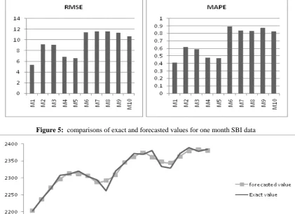
Figure 3: Error comparisons of SBI data for 1 month prediction

For the comparison of the proposed methods we consider the two standard error measures: Root Mean Square Error (RMSE) and Mean Absolute Percentage Error (MAPE). Let 𝑦𝑦(𝑡𝑡) be the actual value and 𝑓𝑓(𝑡𝑡) the forecasted value. Then these measures are defined as

𝑅𝑅𝑀𝑀𝑅𝑅𝑅𝑅 =��(𝑦𝑦(𝑡𝑡)− 𝑓𝑓(𝑡𝑡))_𝑛𝑛 2

𝑛𝑛

𝑡𝑡=1

𝑀𝑀𝑀𝑀𝑀𝑀𝑅𝑅=_𝑛𝑛1�|𝑦𝑦(𝑡𝑡)− 𝑓𝑓(𝑡𝑡)|_𝑛𝑛 × 100

𝑛𝑛

𝑡𝑡=1

These error measures are applied to the time series data. Based on these measures we compare the all proposed wavelet based methods. First we predict one month values using proposed methods. Then it is extended to three month and one year. For one month we calculate RMSE and MAPE which are shown in figures 3 and figure 4.

Figure 4: Error comparisons of ICICI data for 1 month prediction

Figure 5: comparisons of exact and forecasted values for one month SBI data

We compare all these wavelet-based prediction results. From both graphs (Figure3 and Figure 4) it is clear that the methods where SMA is considered are superior to those with variants Exponential smoothing. All methods except 𝑀𝑀₁ and 𝑀𝑀₆ are based on different extensions of different approximations and details levels. The detail parts 𝑑𝑑₁ and 𝑑𝑑₂ are neglected in 𝑀𝑀₂, 𝑀𝑀₄, 𝑀𝑀₇ and 𝑀𝑀₉ respectively. These scales could be noise as they have no great impact on the quality. Figures 3 and 4 show that with respect to the root mean square error 𝑀𝑀₁ and 𝑀𝑀₄ are the best methods and to mean absolute percentage error 𝑀𝑀₁ and 𝑀𝑀₅ performs best. Also methods 𝑀𝑀₂ -𝑀𝑀₅ are better than 𝑀𝑀₆ -𝑀𝑀₉. It means that for the analysis of the approximation level 𝑎𝑎₃ moving average is better than for the exponential smoothing. As a summary we find that 𝑀𝑀₁ shows best performance with respect to both measures. Figure 6 and 7 presents the comparisons of exact values and forecasted values of SBI and ICICI respectively by method by 𝑀𝑀₁. It can be seen that in both type of data predicted values are close to exact values.

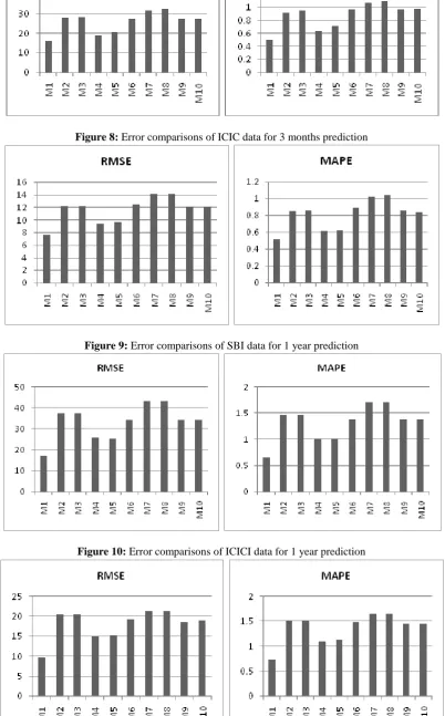
Figure 7: Error comparisons of SBI data for 3 months prediction

Figure 8: Error comparisons of ICIC data for 3 months prediction

Figure 9: Error comparisons of SBI data for 1 year prediction

5. CONCLUSION

In the present work, different prediction methods based on wavelet have been discussed. Wavelet transform decomposes the original time series data in a hierarchy of new time series that behave better than the original time series. The decomposed time series can be predicted more accurately. Here we have used the Indian banking stock prices as an example to show the benefits of using wavelet transform in time series analysis. In this paper we use ten various statistical methods (shown in table 1) on the decomposed parts to extend the data for required period. The computational results show that method 𝑀𝑀₁ which is based on moving average gives best result as compared to other methods.

6. ACKNOWLEDGEMENT

The authors are thankful to Council of Scientific and Industrial Research (CSIR), New Delhi for providing the financial assistance for the preparation of manuscript.

REFERENCES

1. Abiyev H .R. Abiyev H. V (2012). Differential Evaluation Learning of Fuzzy Wavelet Neural Networks for Stock Price Prediction. Journal of Information and Computing Science Vol.7, p. 121-130.

2. Conejo, A., Plazas, A. M., Espinola, R. and Molina, A. (2005). Day-Ahead Electricity Price Forecasting using the wavelet transforms and ARIMA models. IEEE Trans. Power Syst., vol. 20, no. 2.

3. Deora, R. (2013). Time-Scale Comovement between the Indian and World stock markets. The Journal of Applied Business Research Vol.29, p. 765-775.

4. Gencey, R., Selcuk, F., Whitcher, B. (2001). Scaling properties of foreign exchange volatility. Physica A: Statistical Mechanics and its Applications, Vol. 289(1-2), p. 249-266.

5. Gencay, R., Selcuk, F. and Whitcher, B. (2001). An Introduction to Wavelets and Other Filtering Methods in Finance and Economics. San Diego, CA: Academic Press.

6. Gallegati, M. (2008). Wavelet analysis of stock returns and aggregate economic activity. Computational Statistics and Data Analysis, Vol. 52(6), p. 3061-3074.

7. Kim, S., In F. (2005). The relationship between stock returns and inflation: new evidence from wavelet analysis. Journal of Empirical Finance, p. 435-444.

8. Kumar, J. and Manchanda, P. (2010). Prediction for the time series of BSE 100 using wavelets and Neuro-fuzzy approach. Indian Journal of Industrial and Applied Mathematics. Anamaya, New Delhi.

9. M. Pablo, L. Roman (2014). Interest rate changes and stock returns in Spain: A wavelet analysis. Business Research Quality 18, 95-110.

10. Ramsey J. B. (2002). Wavelets in economics and finance: past and future. Studies in Nonlinear Dynamics Econometrics, p. 1-27.

11. Siddiqi A. H. (2004). Applied Functional Analysis: Numerical Methods, Wavelet Methods, and Image processing. Marcel Dekker, Inc., New York.

12. Weinreich I, Rickert H, Lukaschewitsch M. (2003). Wavelet based time series prediction for air traffic data. SPIE International Symposium on Photonics Technologies for Robotics, Automation and Manufacturing.

Source of support: Council of Scientific and Industrial Research (CSIR), New Delhi, India. Conflict of interest: None Declared

[Copy right © 2016. This is an Open Access article distributed under the terms of the International Journal of Mathematical Archive (IJMA), which permits unrestricted use, distribution, and reproduction in any medium, provided the original work is properly cited.]