Proceedings of the
Ninth International Workshop on
Graph Transformation and
Visual Modeling Techniques
(GT-VMT 2010)
Stochastic Graph Transformation with Regions
Paolo Torrini, Reiko Heckel, Istv´an R´ath and G´abor Bergmann
15 pages
Guest Editors: Jochen K ¨uster, Emilio Tuosto
Managing Editors: Tiziana Margaria, Julia Padberg, Gabriele Taentzer
Stochastic Graph Transformation with Regions
Paolo Torrini1, Reiko Heckel2, Istv´an R´ath3and G´abor Bergmann4
1[email protected] 2[email protected]
University of Leicester
3[email protected] 4[email protected]
Budapest University of Technology and Economics
Abstract: Graph transformation can be used to implement stochastic simulation of dynamic systems based on semi-Markov processes, extending the standard approach based on Markov chains. The result is a discrete event system, where states are graphs, and events are rule matches associated to general distributions, rather than just exponential ones. We present an extension of this model, by introducing a hierarchical notion of event location, allowing for stochastic dependence of higher-level events on lower-higher-level ones.
Keywords:Graph Transformation, Stochastic Simulation, Topology
1
Introduction
Graph transformation combines the idea of graphs as a universal modelling paradigm with a
rule-based approach to specify the evolution of systems [KK96]. Behaviour can be modelled
in terms of labelled transition systems, where states are graphs and rule applications represent transitions. A discrete event system can be generally obtained by interpreting rule matches as events. Hierarchical graphs can be used to keep into account the spatial structure of graphs in terms of topological grouping, with advantages that have been underlined from the point of view
of modelling and verification [BL09].
Stochastic graph transformation is applicable to probabilistic analysis and stochastic valida-tion of graph-based modelling. Stochastic simulavalida-tion can be particularly useful as validavalida-tion technique when systems are too complex to be model-checked. It can be implemented relying on
a discrete event system approach [CL08]. Transitions are labelled by scheduling times, randomly
chosen according to given probability distributions — thus replacing stochastic determinism for indeterminism in the models.
A simple form of stochastic graph transformation can be obtained by associating rule names
with exponential distributions [HLM06]. The associated Markov-chain analysis has been applied
to integrated modelling of architectural reconfiguration and non-functional aspects of network
models [Hec05]. However, this approach has some limits. Exponential distributions can express
well the relative speed of processes, but are less than suited to describe phenomena characterised by mean and deviation. Generalised stochastic graph transformation can answer this problem,
with rule matches [HT10,KTH09]. In the latter case, assignment of probability distributions to events may depend e.g. on attributes of match elements. Generalised semi-Markov processes provide the discrete event semantics for such systems.
In reality, events can often be described at different levels of spatial and causal detail. The ex-pression of causal dependency in graph transformation depends solely on rules and their match-ing. On the other hand, in the approaches that we have considered up to now, each event is treated as stochastically independent from any other with respect to the assignment of proba-bility distributions. Stochastic dependency on global variables and derived attributes has been
considered [HT10]. Even allowing that, it is not generally possible to express in a direct way e.g.
that the probability of a certain event depends on other events. This can make it particularly hard to model aspects that involve correlation between different levels of description, as in the case of geographic and biochemical systems, where information is usually found at different levels of
spatial granularity [TSB02].
In this paper we propose an approach based on hierarchical graphs in order to introduce local-isation and granularity of events, we define a notion of structured stochastic simulation allowing us to express stochastic dependency of higher-level events on lower-level ones, and we provide a semantics for it in terms of discrete event systems. Regardless of the specific approach, a major stumbling block in the implementation of stochastic simulation based on graph transformation is the need to compute all the matches at each step. This is hard in principle — the subgraph homomorphism problem is known to be NP-complete, though feasible in many cases of interest. However, the cost of recomputing can be prohibitive. For this reason, we rely on incremental
pattern matching based on a RETE-style algorithm as implemented in VIATRA [BHRV08] (a
model transformation plugin of Eclipse). In [THR10] we presented GRASS, a tool that extends
VIATRA with a stochastic simulation control based on the SSJ libraries [LMV02]. By using a
decoupled notion of graph hierarchy, it should be possible to implement hierarchical stochastic simulation in VIATRA/GRASS.
1.1 Hierarchical extensions
Hierarchy in graph models can be used to introduce a notion of topological grouping on model elements. Grouping information can be represented as a hierarchy graph, as distinct from the
un-derlying graph, relying on a decoupled approach [BKK05]. In the case of bigraphs, the approach
is to pair place graphs and link graphs, together with a specific notion of matching [Mil08].
Here we use topology to localise events, rather than elements, relying on a generic notion of rule matching. A model consists of an underlying graph coupled with a place graph, where the latter
is a directed acyclic graph (dag) from which the hierarchy arises, as partial order (≤).
Topo-logical grouping arises from rule matching through the hierarchy. Nodes in thedag are places
and edges represent containment between places (hierarchical containment). The two graphs are
linked together by containment edges (coupling containment) that map underlying graph nodes
to places. Regions are defined as downward-closed sets with respect to the hierarchy, i.e. closed
sets in the corresponding order topology [TSB02].
number of enabled matches of a certain type — what we call a density measure; (2) on the
scheduling of other events — what we call anactivitymeasure. In this way, we expect to be able
to perform more sensitive stochastic analysis without resorting to making models and reachabil-ity analysis more complex.
In fact, density measures boil down to counting matches, therefore they could be handled by introducing additional attributes in a flat model — though this would mean making the model more complex. Activity measures are trickier, as in principle they might lead to circular depen-dencies. This is avoided by requiring that stochastic dependency between events as well as event time scheduling comply with the hierarchy. Therefore, no event may depend on higher level ones, and at each step of the simulation, the time scheduling of lower-level events takes place before that of higher-level ones.
2
Example
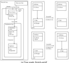
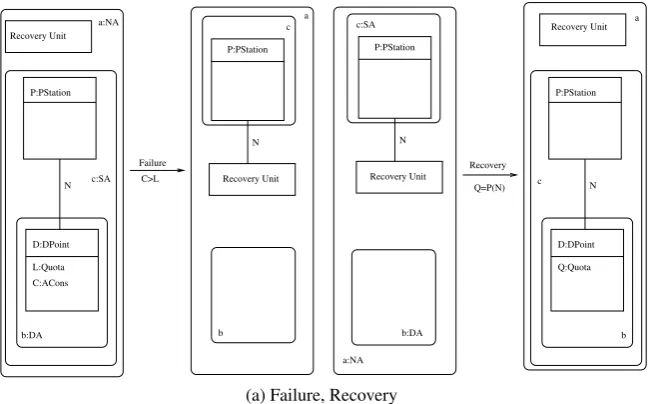
We model a power grid as example in which higher-level events may depend stochastically on large numbers of lower-level ones. Each power source serves a number of distribution points, by allocating power quotas in a reconfigurable way. Appliances can be added to and removed from a distribution area, and they can be connected to and disconnected from distribution points, determining the level of consumption, which must remain within a tolerance of the quota. A power failure may occur when the quota is overstepped. A failure determines the disruption of the distribution point, with consequent loss of data, and it forces the intervention of a recovery unit. Actual reconfiguration is carried out following optimisation criteria that can be reflected stochastically in the application of the rule.
The model is based on the SPO approach, and uses typed graphs with attributes. A power station is connected to each of the distribution points by power lines denoted by multi-edges, i.e. sets of parallel edges represented as a single edge with an integer value. A station can reconfig-ure the capacity of each power line depending on the available power and the distribution area consumption — this takes place by changing the number of line edges, also updating residual power and local quota.
The spatial structure of the model is quite simple — there are three types of places: thenetwork
area, asupply areafor each station, and adistribution areafor each service point. Each place is
represented as a rounded box. The hierarchy order≤is represented as containment (larger boxes
are places higher up in the order, therefore associated with higher-level elements). The coupling order is also represented as containment in an obvious way — each underlying graph node (a square box) being coupled only with the smallest place box it is contained in. In this example,
the place graph is a tree. The notation could be easily extended to thedagcase, by associating
places to intersections. The symbolsDec,Inc,Tol,Add,F,G,H,Pin the figures stand for given
functions.
SwitchOff D:DPoint A:App D:DPoint A:App C2=Dec(C1,X) C1:ACons X:CWeight C2:ACons D:DPoint A:App C2=Inc(C1,X) D:DPoint A:App SwitchOn C1:ACons L:Quota C2:ACons X:CWeight C2<Tol(L) Distribution Point Appliance Residual Power: Int Overlay Line Area Recovery Unit Quota: Int Area Distribution Area Connection Supply Cons: Int Cons Line N:Int N:Int a a Network Area a:DA a:DA Power Station Weight:[Int]
(a) Type graph, Switch-on/off
Figure 1: Type graph, Switch-on/off
N M
D:DPoint D:DPoint
Reconfiguration
M = F(R1,
P:PStation P:PStation R1:ResPower R2:ResPower L1:Quota L2:Quota X:CWeight A:App A:App Add(X) Remove a b a a:DA a a:DA b:DA a:SA C:ACons C,N) L2 = G(L1,N,M) R2= H(R1,N,M)
(a) Reconfiguration, Add, Remove
Failure Recovery Q=P(N) N
Recovery Unit P:PStation
D:DPoint N P:PStation
D:DPoint Recovery Unit
N P:PStation
N Recovery Unit
P:PStation
Q:Quota L:Quota
C:ACons
C>L
a
b c
a
b c
b:DA
c:SA Recovery Unit
b:DA c:SA a:NA
a:NA
(a) Failure, Recovery
Figure 3: Failure, Recovery
as adding appliances, switching on and failure, may be assigned exponential distributions. Ac-tions more plausibly associated with mean values, such as switching off and recovery, may be more naturally associated with normal distributions. Crucially, reconfiguration can dependent stochastically on the context.
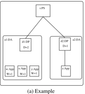
In the example, there are two possible matches for the reconfiguration rule — one witha1 and
the other witha2 as distribution areas. In order to model stochastically a “smart” reconfiguration
strategy, one could make the probability of application inversely dependant on the difference between quota and area consumption (a derived attribute associated with distribution points and
denoted byDin the picture). However, if that is to be the only criteria, here there is little chance
of modelling a high quality of service without changing the model. Given a high rate of switching
on against a low one of appliance addition, the area a1 is more at risk than a2, in spite of the
higherDvalue. This risk is essentially associated with the number of matches forswitch onin
a1, and further than that — with their scheduling times.
Of course it would be possible to retain information about the number of appliances in an area explicitly, by adding an attribute — however, apart from the need to extend the model, this way of capturing the density measure would not be the most natural in this case, as it would not belong to the service point. Moreover, it is difficult to think of a similar way to capture an activity measure. On the other hand, the knowledge embedded in the reconfiguration strategy might be based on estimates rather than precise data. Therefore, modelling it in terms of implicit stochastic dependence seems realistic.
3
Stochastic Graph Transformation
Stochastic graph transformation for semi-Markov process modelling requires us to track matches
y:App s:PS
W=1 a1:DA
x:App W=1 W=1 w:App
a2:DA d2:DP
D=1 d1:DP
D=2
z:App
(a) Example
Figure 4: Example
matches. Here we provide a general definition of typed graph transformation that supports track-ing with respect to a generic approach (although the runntrack-ing example is based on SPO), allowtrack-ing for node type inheritance and negative application conditions. We then extend the notion, by en-dowing graphs with hierarchy and derived topological structure.
3.1 Graph transformation
In existing axiomatic descriptions of graph transformation [KK96], a graph transformation
ap-proach is given by a class of graphs G, a class of rules R, and a family of binary relations
⇒r⊆G×G representing transformations by rulesr∈R. Here we assume that each rule r is
associated to a left hand-side graph Lr and a set of negative application conditions Nr. This
notion can be further refined by introducing a definition of rule match depending on a given ap-proach (including SPO and DPO). In the following, we will sometimes use a syntax for function
definitions with dependent types [Bar92] in a comparatively informal way, in order to specify
functions that we assume to be implementable, by writingΠx∈α.β rather than α→β when
x∈α andβ depends onx.
Basically, a graph is a tripleG=hNodesG,EdgesG,asgGi, where forx∈NodesG,asgG(x) =
hy,zi withy,z∈NodesG. At an abstract level, a partial match of a rule r in a graphGcan be
represented as a triplem=hr,g,ci, wherer=rule(m),g=SG(m)is a partial graph morphism
fromLr intoG, andc=AC(m)⊆Nr is the set of application conditions that are satisfied. We
denote the graph elements of the match, i.e. the image ofm, byEL(m). We say that a matchm
isvalidwhenSG(m)is total andAC(m) =Nr. We denote byMr,Gthe set of the partial matches
ofr inG. Mr,G is ordered by a relationvr,G, component-wise defined as subgraph and subset
relation on theSG and ACcomponents of the matches, respectively. We define the set of all
partial matches in a graphGasMG=Sr∈RMr,G, and byMGv ⊆MG the set of all those that are
valid.
Def. 1 We define a function⇒:ΠG∈G.MGv →G. We writeG⇒mHfor⇒(G)(m) =H, and
we say that this is thetransformation stepdetermined by the application of rulerule(m)
Notice that transformation steps correspond to a function that is partially defined with respect to the set of all matches. The functional requirement captures the idea that rule application is
well-defined and deterministic once a valid matchm is found in G. This is needed, in order
to guarantee that matches form a proper set, unlike in more abstract presentations [EEPT06].
Also notice that, however, we implicitly allow for a global renaming action associated with a transformation.
Def. 2 A graph transformation system (GTS) G=hR,G0i consists of a set R⊆R of rules
and an initial graph G0∈G. A transformation in G is a sequence of rule applications
G0⇒m1 G1⇒m2· · · ⇒mn Gnusing rules inGwith all graphsGi∈G.
Assuming finite graphs and an enumerable set of rules, the graphs that are reachable fromG0
by a finite sequence of transformation steps form a set, denoted byLG, and so do the partial
matches over the reachable graphs, denoted byMG.
Even without fixing the approach, we can say that in general, a transformation stept=G⇒m
His associated with a setDeltof all the graph elements that are deleted or modified byt, and with
a setCret of all the graph elements that are created byt. Correspondingly, the partial matches
that are destroyed form a setDG,t ⊆MG, those that are created form a setCH,t⊆MH, and those
that are preserved areM|t=MG\DG,t. From the deterministic assumption,MH=σt(M|t)∪CG,t
follows, whereσt is the renaming induced byt(assuming the name spaces are disjoint).
We are interested in defining a notion of persistent match, by identifying matches that are preserved through transformation. In particular, from the point of view of stochastic models,
givenm1∈σt(DG,t),m2∈DG,t andm2=σt(m1), we want to identifym1 andm2when they are
both valid with respect to the same ruler. This can be generalised to partial matches. In [KTH09,
KL07] we relied on a conservative naming policy — here we adopt a looser one altogether,
though still defining a persistent match as equivalence class.
In order to abstract from renaming, we define, for n1 ∈MR,G0,n2 ∈MR,G00, the symmetric
relationn1=an2that holds whenever for all transformation stepst, ift=G0⇒mG00andn1∈M|t,
thenn2=σt(n1), and ift=G00⇒mG0 andn2∈M|t thenn1=σt(n2). We can then define the
transitive closure using the least fixpoint operator (µ)
n1≡n2=d f µE.(n1=n2)∨(∃n3.E(n1,n3)∧n3=an2)
It is a matter of routine to show that ≡ is indeed an equivalence relation. The persistent
matches over the set of the reachable graphs inGcan therefore be defined as the quotient class
MG=MG/≡. We calleventa persistent valid match, and we denote withEGthe corresponding
set of events. We defineMG={[m]|m∈MG}, andEG={[m]|m∈MGv}. This in general will
allow us to lift definitions from valid matches to events.
Lr n1 //
=
n2
8
8
G t /H
3.2 Hierarchical structure
We use hierarchical graphs in the decoupled sense [BKK05], i.e. we define a hierarchical graph
as graph that includes the underlying graph as well as a directed acyclic graph representing the hierarchical structure.
Def. 3 A hierarchical graph is a graphGin which there is a distinguisheddag PG⊂Gcalled the
place graph, where the nodes ofPGare theplaces;
(a) the edges that link nodes inG\PGto (non-empty) places, calledC-edges, express
cou-pling containment and form a distinguished setCEdgesG⊂EdgesG;
(b) the edges connecting places together (H-edges) express hierarchical containment.
Moreover, the following conditions must be satisfied:
(1)hPG,≤Giis a partial order (hierarchyofG), where≤Gis the reflexive-transitive closure
of hierarchical containment.
(2)<Gis downward well-founded (i.e. there are no infinite descending chains).
(3)≤Ghas finite degree (i.e. it is finitely branching).
In addition, (i) theunderlying graphofGis defined as the largest subgraph ofGwhich
does not contain either nodes or C-edges — this may be expressed set-theoretically as
UG= (G\PG)\CEdgesG;
(ii) forX ⊆NodeG,locG(X)denotes the finite set of the places associated to any element
ofX by C-edges (thelocationofX); we also writelocG(x)forlocG({x}), andlocG(m)for
locG(ELG(m)∩NodesG)withm∈MG.
We say thatGiscompletewhenever for each nodexinUG,locG(x)6= /0.
We say thatGisgroundedwhenever for each nodexinUG,locG(x)contains at most one
element.
We denote byGhthe class of the hierarchical graphs, byGcthe class of the complete ones,
byGgthat of the grounded ones, and byGcgthat of the complete grounded ones.
Clearly, PG may be a finitely branching tree. In practice, PG is going to be mostly finite
— indeed, assuming≤G does not contain infinite ascending chains and has a finite number of
minimal elements, finiteness follows, using Koenig’s lemma.
Any partial order≤can be associated to an Alexandroff topology where the downward-closed
sets are the closed sets and≤coincides with the specialisation order [Vic89]. This is too
fine-grained though, as there is no need to consider downward-closed sets which are not generated by matches, and we prefer to take nodes that share a place to the same region. Therefore we define the following.
Def. 4 Given a partial matchm∈MG, we say that thegraph regionofm, denoted bygregG(m),
is the smallest subgraphJ⊆Gsuch that
(1) set-theoretically, SG(m) ⊆J, locG(m)⊆J, and all the C-edges and H-edges in G
between elements ofJ are inJ.
(2)Jis downward-closed with respect to≤G, i.e. forw,zplaces inPG, ifw∈Jandz≤Gw
thenz∈J
(3) for each nodexinG, iflocG(x)∩J6=/0 thenlocG(x)⊆J.
We denote byRegGthe set of the abstract regions defined onMG.
Form,m0∈MG, p∈RegG, we say thatmislocatedinpiffregG(m)⊆p. We say thatm
islower-levelwith respect tom0(resp.m0ishigher-levelwrtm) and we definem<Gm0iff
regG(m)⊂regG(m0).
Notice thatm⊆m0follows fromEL(m)⊆EL(m0)for anym,m0∈MG. Set-theoretically, it is
not difficult to see thatRegG is closed with respect to arbitrary intersection (condition 3 helps).
Adding empty and global region, we may regardRegGas basis of an Alexandroff topology, where
the specialisation order is monotonic with respect to≤G. From the downward well-foundedness
of<G, it follows that <G is similarly well-founded, i.e. it has no infinite descending chains.
Abstract regions can therefore be used to order events.
We can now introduce a notion of hierarchical transformation system, consistently with the
generic approach, along the lines of the definitions1,2, by adapting them to classes of
hierarchi-cal graphs. We takex=h|c|g|cg.
Def. 5 Ahierarchical transformation step functionis a function⇒x:
ΠG∈Gx.MGv →Gx such
that (by the notation of def.1),G⇒x
mHiffG⇒mH, providedG,H∈Gx.
A hierarchical graph transformation system (HGTS)G=hR,G0iconsists of a setR⊆R
of rules and an initial graphG0∈Gx.
A transformation inG is a sequence of rule applications using rules inGand applying
them through⇒x.
In case ofx=h, the definitions are clearly generalisations of those forG. The running example
is meant to be a case of x=cg. Notice that in every case, the notion of match is implicitly
assumed to be the most general — this can be stated by saying that for every matchm∈MG,
SG(m)∈Gh. However, in order to keepE
Gfinite, we assume as fixed the names of empty places
that are preserved by the transformation.
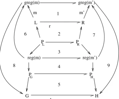
When the system is based on the SPO approach — as in the running example, each rule can be defined in terms of two components — one defined on the underlying graph, the other on the
place graph. Figure6 provides with a diagrammatic illustration, where 1–5 are pushouts and
6–9 are pullbacks. Notice that regions can be used to wrap the side-effects of SPO rules — e.g. theFailure rule in the running example, where all the line edges which are deleted are in fact between nodes that are included in the supply area — thus generally allowing for more modular transformations.
3.3 Stochastic Modelling
Generalised stochastic graph transformation has been defined in [HT10,THR10, KTH09], by
associating events with general distributions, each of them expressed as a cumulative distribution
function (cdf) — i.e. a function from real numbers to probability values. Here we denote by
Dist(e)⊆Real→[0,1]the type of thecdf assigned to evente.
Def. 6 A generalised stochastic graph transformation system (GSGTS) is a structureS=hG,∆0i
whereGis a GTS,∆0:Πe∈EG.Dist(e)is a distribution assignment, which associates with
L R
H G
P
L PR
P
G PH
t 1
3 2
4
5
6 7
8 9
m
r
m’
greg(m) greg(m’)
reg(m) reg(m’)
Figure 6: hierarchical transformation
The behaviour of a GSGTS can be described as a stochastic process over continuous time, where reachable graphs form the state space and the application of transformation rules defines state transitions as instantaneous events. More precisely, a rule enabled by a match defines an
event associated with an independent random variable (timer, or scheduling time) which
repre-sents the time expected to elapse (scheduled delay) before the rule is applied to the match. As
the simulation is executed, the timer is randomly set according to the static specification
pro-vided by thecdf of the corresponding event — in the implementation, this involves a call to a
pseudo-random number generator (RNG).
We intend to extend the definition of stochastic graph transformation in order to make it
pos-sible to express the dependency of the probability distribution of an eventeon other events, and
more precisely on properties of the graph, such as the number of events of a certain type in a
certain region associated toe, or the average scheduled delay for lower-level events of a certain
type — e.g. the dependency of thecdf ofReconfigurationevents on the number and the
sched-uled delay ofAdd andSwitchOn events in the relevant distribution area, given in the running
example. Syntactically, we also allow for rule constructors over finite domains, i.e. c:X →R
withX finite, representing a set of rulesr1=c(x1), . . . ,rk=c(xk), wherekis the cardinality of
X — e.g.Add(X)in the example.
We now consider stochastic simulation from the point of view of a HGTS G. For each G∈
LG, we can assume to have a scheduling function
schedG:Πe∈EG.Dist(e)→Time(e)
which assigns a value to each timer, given itscdf — whereTime(e)⊆Realis a subtype of the
reals that represents a random variable. We can also assume to have an event counting function
countG:Πp∈RegG.Πr∈R.Num(r,p)
whereNum(r,p)⊆Nat is a subtype of the naturals that represents the number of matches of
Once we assume that for each stateG, the scheduling of delays follows the granularity order
<G, we can allow for thecdf of an evente∈EGto depend
(1) on the general number of events inG, i.e. on{countG(r,p)|r∈R,p∈RegG}, and as a special
case, on the number of events located in the same region, i.e. {countG(r,regG(e))|r∈R}(local
density);
(2) on the scheduled delays of lower-level events, i.e. on{schedG(e0)|e0<e}(local activity).
We now show how the distribution assignment can be functionally defined, in order to make
the above possible. We can associate local density tolocal event counting, specified as function
of type
LDensG=d f Πe∈EG.Πr∈R.Num(r,regG(e))
We can associate local activity to a notion oflocal delay scheduling, specified as a function of
type
LActG=d f Πe1e2∈EG.e2<Ge1→Time(e2)
We can then introduce a notion of abstract distribution assignmentδ that depends on both,
specified as follows
δ:ΠG∈LG.Πe∈EG.(LDensG(e)×LActG(e))→Dist(e)
Partial schedulingπG:Πe∈EG.LDensG(e)×LActG(e)can now be defined by recursion
(as-sumingδ is given)
πG=d f µf.λe1.(λr.countG(r,regG(e1)),λe2.ife2<Ge1then(schedG(e2)(δ(G)(e2)(f(e2))))
Finally, the distribution assignment∆:ΠG∈LG.Πe∈EG.Dist(e)can be defined as
∆=d f λG.λe.δ(G)(e)(πG(e))
This shows that∆can be defined recursively, givensched,count,δ, and relying on the
well-foundedness of<.
Def. 7 A stochastic hierarchical graph transformation system (SHGTS) is a structure H=
hG,δi, where G is a HGTS and δ is a function specified as above, so that ∆ :
ΠG.Πe.Dist(e)can be defined as the function that assigns a continuouscdf to each event
for each reachable graph.
4
Stochastic Simulation
We define an operational interpretation of SHGTS in terms of semi-Markov processes, following
an approach already used in [THR10,KTH09,KL07]. We rely on a representation of stochastic
Semi-Markov processes are continuous-time stochastic processes in which the embedded jump chain is a Markov chain and the inter-event times are associated with general distribu-tion funcdistribu-tions. This means that events are independent of past states, but may depend on the time spent in the current one. They are a generalisation of continuous-time Markov processes, which allows only for exponential distributions. More formally, a semi-Markov process can be
defined as a process generated by ageneralised semi-Markov scheme(GSMS) [DK05]. Here we
need to define a structure that is syntactically more general than a GSMS, insofar as we need to keep hierarchy and delay scheduling order into account.
Def. 8 Ahierarchical semi-Markov scheme(HSMS) is here a structure
P = hZ,E,enabled:Z→℘(E),vS:Z→(E×E)→Boolean,
new:Z×E→Z, cdfAsg:Z→E→Real→[0,1],s0:Zi
where Z is a set of system states; E is a set of timed events; enabled is the activation
function, so thatenabled(s) is the finite set of active events associated with states;new
is a partial function depending on states and events that represent transitions; cdfAsg is
the distribution assignment, so thatcdfAsg(s)(e)gives acdf of the scheduled delay ofeat
states;vS(s)is a well-founded order (schedule-making order) on the enabled events at
states; ands0is the initial state.
Def. 9 Given a SHGTSH=hR,G0,δi, we define its translation to an HSMSPHas follows:
1. Z=L(hR,G0i)i.e. set of graphs reachable fromG0by rules inR
2. E=EGi.e. the set of possible events forG=hR,G0i
3. enabled(G) =EGi.e. set of all events enabled in graphG
4. new(G,e) =HiffG⇒eHi.e. transition is defined as transformation
5. cdfAsg(G)(e) = ∆(G)(e)
6. vS(G) =v
G
7. s0 = G0
This embedding can be used as static framework for the definition of a simulation algorithm that is adequate with respect to system runs, in the sense that there is a one-to-one correspon-dence between the runs of the original SHGTS and those of the resulting HSMS, and therefore correct and complete with respect to reachability. The algorithm, based on the general scheduling
scheme given in [CL08], can be described as follows.
1. Initial step
(a) The simulation time is initialised to 0.
(b) The set of the enabled eventsA=enabled(s0)is computed.
(c) The schedule-making ordervS(s
(d) For each evente∈A, a scheduling timeteis determined by RNG depending on the
probability distribution functioncdfAsg(e)(s0);
(e) The enabled events with their scheduled times are collected in the event list ls0 =
{(e,te)|e∈A}ordered by time values.
2. For each successive step — given the current state s ∈Z and the associated event list
ls={(e,t)|e∈active(s)}
(a) the first elementk= (e,t)is removed fromls;
(b) the simulation timetSis updated by increasing it tot;
(c) the new states0is computed ass0=new(s,e);
(d) the listms0 of the surviving events is computed, by removing fromlsall the disabled
elements, i.e. all the elements(z,x)oflssuch thatz∈/enabled(s0);
(e) The schedule-making ordervS(s0)is computed.
(f) a listns0 of the newly enabled events is built, containing a single element(z,tz)for
each eventzsuch thatz∈enabled(s0)\enabled(s)and is scheduled at timetz=tS+
dz, wheredzis the random delay value given by RNG depending on the distribution
functioncdfAsg(s0)(z);
(g) the new event listls0 is obtained by reordering the concatenation ofms0 andns0 with
respect to time values
Part of the complexity of the algorithm is hidden in the recursive definition ofcdfAsg, which
means that time scheduling takes place following the schedule-making order<S, associated to
<Gby the translation. The translation and the assumptions on the hierarchy≤also guarantee that
<S(s)is well-founded. Essentially, the algorithm relies on graph transformation with persistent
matches, on functions to count events, and on ordered delay scheduling implemented as calls to RNG.
5
Further work
Expressing stochastic dependencies associated with density and activity measures — as in the example — can be useful to model situations in which specific events depend on large num-bers of co-located ones, as in describing biochemical processes at different levels of detail (e.g. molecular and cellular). Graph transformation can be good at tracking individual processes — however, there are aspects that can be modelled more efficiently in terms of mass effect and
dif-ferential equations [Car08]. Therefore, the general capability of expressing presence of reactants
and reactions in a region can be useful.
From the point of view of an implementation, applying few high-level rules rather than many low-level ones could ease the cost of updating incremental data-structures. As presently
imple-mented in GRASS [THR10], scheduling is carried out independently of the RETE network. This
might make hierarchical scheduling comparatively expensive. Hierarchical information could be
handled more efficiently by introducing a further level of incrementality based on alive
the transformation context, so that changes to the spatial structure can be instantly mapped to the underlying graph.
6
Conclusion
Stochastic simulation is a promising field of application for graph transformation techniques. We have argued that structured graphs can be useful for stochastic simulation. We have focussed on probabilistic dependency of events on global and local properties, in order to make stochastic modelling more flexible. In particular, we have shown that hierarchy can be used to define a topological order on events, allowing for the introduction of a weak notion of modularity and an increased expressiveness with respect to stochastic simulation. This extension can be embedded in discrete event models of stochastic processes. We think that an implementation of stochastic simulation along this lines can take benefit from an appropriate use of incremental pattern-matching.
References
[Bar92] H. P. Barendregt. Lambda Calculi with Types. In Abramsky et al. (eds.),Handbook of
Logic in Computer Science. Volume 2, pp. 117–309. Oxford – Clarendon Press, 1992. [BHRV08] G. Bergmann, A. Horv´ath, I. Rath, D. Varr´o. A benchmark evaluation of
incremen-tal pattern matching in graph transformation. InInternational Conference on Graph
Transformation. LNCS 5214, pp. 396–410. 2008.
[BKK05] G. Busatto, H.-J. Kreowski, S. Kuske. Abstract hierarchical graph transformation.
Mathematical Structures in Computer Science15(4):773–819, 2005.
[BL09] R. Bruni, A. Lluch Lafuente. Ten Virtues of Structured Graphs. InGT-VMT’09. 2009.
[Car08] L. Cardelli. Artificial Biochemistry. In Springer (ed.), Algorithmic Bioprocesses.
LNCS, 2008.
[CL08] C. G. Cassandras, S. Lafortune.Introduction to discrete event systems. Kluwer, 2008.
[DK05] P. R. D’Argenio, J.-P. Katoen. A theory of stochastic systems part I: Stochastic
au-tomata.Inf. Comput.203(1):1–38, 2005.
[EEPT06] H. Ehrig, K. Ehrig, U. Prange, G. Taentzer. Fundamentals of Algebraic Graph
Transformation (Monographs in Theoretical Computer Science. An EATCS Series). Springer, 2006.
[Hec05] R. Heckel. Stochastic Analysis of Graph Transformation Systems: A Case Study in
P2P Networks. InProc. Intl. Colloquium on Theoretical Aspects of Computing
(IC-TAC’05). LNCS 3722, pp. 53–69. Springer-Verlag, 2005.
[HLM06] R. Heckel, G. Lajios, S. Menge. Stochastic graph transformation systems.
[HT10] R. Heckel, P. Torrini. Stochastic Modelling and Simulation of Mobile Systems. 2010. to be published.
[KK96] H.-J. Kreowski, S. Kuske. On the Interleaving Semantics of Transformation Units
- A Step into GRACE. In Cuny (ed.), Graph Grammars and their Application to
Computer Science. Pp. 89 – 106. Springer, 1996.
[KL07] P. Kosiuczenko, G. Lajios. Simulation of generalised semi-Markov processes based
on graph transformation systems.Electronic Notes in Theoretical Computer Science
175:73–86, 2007.
[KTH09] A. Khan, P. Torrini, R. Heckel. Model-based Simulation of VoIP Network
Recon-figurations using Graph Transformation Systems. In Corradini and Tuosto (eds.),Intl.
Conf. on Graph Transformation (ICGT) 2008 - Doctoral Symposium. Electronic Com-munications of the EASST 16. 2009.
[LMV02] P. L. L’Ecuyer, L. Meliani, J. Vaucher. SSJ: a framework for stochastic simulation in
Java. InProceedings of the 2002 Winter Simulation Conference. Pp. 234–242. 2002.
[Mil08] R. Milner. Bigraphs and Their Algebra.Electr. Notes Theor. Comput. Sci.209:5–19,
2008.
[RBOV08] I. Rath, G. Bergmann, A. Okr˝os, D. Varr´o. Live model transformations driven by
incremental pattern matching. InICMT’08. LNCS 5063, pp. 107–121. Springer, 2008.
[THR10] P. Torrini, R. Heckel, I. R´ath. Stochastic Simulation of Graph Transformation
Sys-tems. InFASE’10. Pp. 154–157. 2010.
[TSB02] P. Torrini, J. G. Stell, B. Bennett. Mereotopology in second-order and modal
exten-sions of intuitionistic propositional logic. Journal of Applied Non-Classical Logic
12(3–4):490–525, 2002.