Quality assurance and Data Validation of the ATLAS Data Challenges Simulation Samples

Quality assurance and Data Validation of the

ATLAS Data Challenges Simulation Samples

J-F.Laporte

_{, J.B.Hansen}

1_{DAPNIA/SPP, CE Saclay, Gif sur Yvette, F-91190 France} 2

CERN, 1211 Geneva 23, Switzerland

Abstract— In 2002 and 2003, a procedure has been developed

and extensively used to validate samples produced at different sites for the ATLAS Data Challenges Phase 1 and Phase 2. This brief note describes the various components of this procedure and serves as a guide to using the actual technical material available on the Web[1].

I. INTRODUCTION

The primary aim of the Data Challenges (DC) Samples Validation is to insure the reproducibility of event samples produced in different simulation sites.

The procedure attempts to establish quantitatively the resemblance of two samples by comparing various distributions. It outputs χ2s from which the resemblance of the samples could be evaluated. As a consequence, it could be used to monitor long run production as well as changes in the simulation.

The procedure is not intended to be a Physics validation: two samples found similar will be similarly correct or similarly wrong. However by comparing new DC samples with old extensively tested samples produced for the ATLAS Physics TDR [2], the procedure permits early detecting of dissemblance, which can be interpreted in terms of detector performance.

We decided to perform reconstruction of the DC samples and to base the comparison on the reconstruction outputs. Given the circumstances when this effort was launched, it was decided to use of ATRECON reconstruction chain and to base the distribution comparisons on the CBNTATRECON n-tuples [3]. Therefore the validation procedure is not testing the official ATLAS Reconstruction chain, i.e. reconstruction in

Athena. However it has some relevance to the reconstruction tests since some of the reconstruction packages that are used here, can be to run both in ATRECON and in Athena.

The procedure material comprises a reconstruction procedure and a PAW analysis procedure.

II. RECONSTRUCTION

A. Framework and Reconstruction packages

The reconstruction procedure uses the former ATLAS reconstruction framework, ATRECON. This framework was extensively used for the ATLAS Physics TDR studies [2] and is capable of running most of the main ATLAS reconstruction packages. It satisfies all the criteria of availability, simplicity, robustness and stability, which are required to build a validation chain for the massively produced DC samples. We decided to run the Fortran Calorimeter reconstruction package which runs in ATRECON only and because they are capable to run both in ATRECON and in Athena, the Inner Detector reconstruction package xKalman[4] and the Muon Spectrometer reconstruction package Muonbox[5].

B. Reconstruction set-up

Most ATLAS collaborators know how to use ATRECON. The reconstruction procedure is by no means innovative. It aims to provide ready and easy to use machinery solving the painful management of inputs and outputs of jobs for the massive reconstruction of huge DC data. Given the size and the rate of DC production, serious attention must be given to these issues from the start, in order to avoid total confusion.

The procedure comprises a series of scripts. They allow the user to cope with the various locations of the events files (on tape, on castor, etc.), to run indifferently in interactive or in batch mode, and to store reconstruction outputs on castor in a standard manner. Configuration parameters allow coping with site-specific features when installing the tool suite outside CERN. In addition a script is provided which automatically generates set of datacards for handling, for instance, events within given ranges or with a list of events excluded.

The procedure was found convenient to handle the reconstruction of several million events, despite the small

ATL-SOFT-2003-003

number of people directly involved in this reconstruction. The produced CBNT_ ATRECON n-tuples of the reconstructed di-jet samples, single e, γ, π, and µ samples at various pT, and H→2γ, H→2e2µ, H→4 µ samples, are available on the Web. Finally, one should note that this large-scale exercise has shown that the stability and the quality of services such as afs, castor, batch system are essential items for successful massive reconstructions and analyses.

III. COMPARITIVE ANALYSIS

The comparative analysis of two samples is semi-automatic and proceeds in two steps. First, predetermined distributions are built from the CBNT ATRECON n-tuple for each sample. Then, distributions from the two samples are automatically compared by computing and by displaying the χ2s and their differences.

A. Event sample distributions

The first step consists in the execution of a master PAW kumac accessing the n-tuples of a given event sample, running an open list of sub-detector specific kumacs and collecting the histograms that they produce.

Access to single n-tuple as well as a set of n-tuples is possible. There is no limitation on the distributions that the sub-detector specific kumacs can build but on the values of the distribution identifiers, which must lie in a range allocated to each kumac. It should be noted that, although the sub-detector specific kumacs do depend on the CBNT ATRECON n-tuple structure, the master PAW module does not. Indeed, its first function, i.e. access to and chaining of bunch of n-tuples, relies on naming convention of the reconstruction outputs, while its second function, i.e. execution of the listed analysis kumacs, does not depend on what the latter actually do. In this sense, this module could be reused for validation of n-tuples of an other type than the CBNT ATRECON n-tuples, e.g. the CBNT Athena n-tuples.

The sub-detector specific analysis kumacs used for the DC1 Phase 1 and 2 validation, have been provided by J. Schieck, D. Barberis and D. Rousseau for the Inner Detector, by A. Kiryunin and J. Beck Hansen for the Calorimeters and by J.-F. Laporte for the Muon Spectrometer.

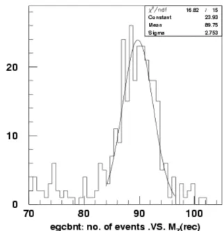
At the end of this step, several tens of distributions, stored in a validation histogram output file, are available for subsequent comparisons. Examples of such distributions are shown in Figure 1 to Figure 4.

B. Two samples Comparison

The last step consists in an automatic histogram-to-histogram comparison performed on the distributions constructed in the previous step.

A single kumac performs these comparisons by using the validation histogram files of the two event samples to be compared. An example of the result for one distribution is shown in Figure 5.

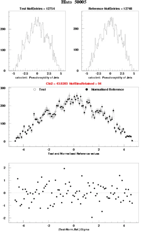
Distributions for the two samples are first displayed separately. Then, in order to study their differences, they are

shown together, the reference sample distribution being rescaled to the number of entries of the other distribution. A bin-to-bin χ2 is then computed and printed out. Finally, the bin-to-bin differences divided by the statistical errors are plotted for each bin1. These displays permit a detailed and quantitative examination of the differences of the distributions.

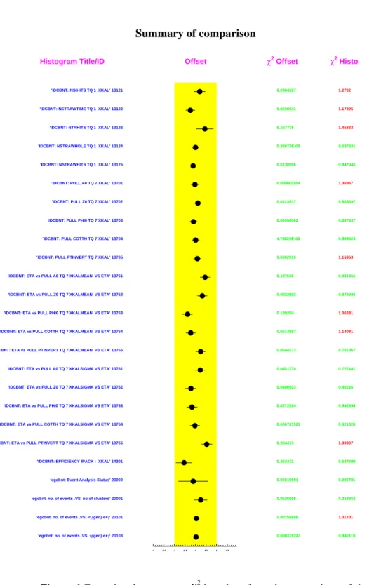
After having compared all available distributions, a summary

χ2

-bar chart is displayed as illustrated in Figure 6. It permits, at a glance, to immediately identify the dissembling distributions among the tens of examined ones.

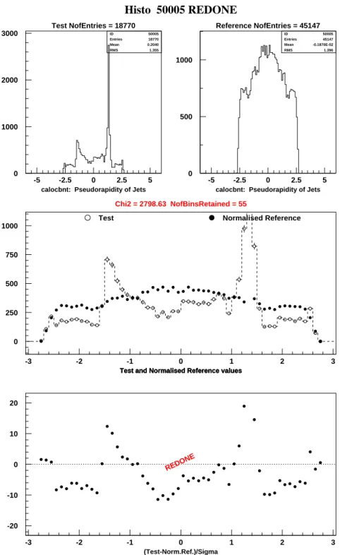
An example of dissembling distributions is shown in Figure 7. In this particular case, a benign but quite spectacular simulation error was responsible.

The comparison kumac, which performs the histogram-to-histogram comparison, is completely independent of the CBNT ATRECON n-tuple structure. Without change, it can be reused to compare any pair of validation histogram files, e.g. those that would be built by analysing CBNT Athena n-tuples.

IV. CONCLUSIONS

The suite of tools presented here turned out to be a key element of the ATLAS Data Challenges production DC1 Phases 1 and 2. It has permitted early detection of problems in the simulation and in site software installation, as well as monitoring of long run production. Although built on

ATRECON reconstruction, it is straightforward to reuse its main components for analysing Athena outputs.

Although it cannot replace the necessary dedicated Physics performance studies [6], the Data Validation Procedure makes it possible to take a first glance at detectors performance evolutions.

ACKNOWLEDGEMENTS

We whish to thank J. Ernwein for his careful reading of this note

REFERENCES

[1] All material described in this note is available on the Web http://atlas.web.cern.ch/Atlas/GROUPS/SOFTWARE/DC/Validation/w ww

[2] ATLAS Physics TDR, CERN-LHCC 99-15

[3] Documentation on CBNT_Atrecon ntuples is available at http://droussea.home.cern.ch/droussea/cbnt/cbnt.html

[4] I. Gavrilenko, “Description of Global Pattern Recognition Program (XKalman)”, ATL-INDET-97-165

[5] M. Virchaux et al, “Muonbox: a full 3D tracking programme for Muon reconstruction in the ATLAS Spectrometer”, ATL-MUON-97-198 [6] B. Epp et al, “Data Challenge 1: Beauty Physics Validation”,

COM-PHYS-2003-003.

1 _{It happens that fluctuations, which are present in a few} bins only, prevent examination of the rest of the distribution. In that case, a tentative rescue “REDONE” procedure is tried once by excluding the concerned bins.

Figure 1 Example of a distribution of the pulls of

the Z0 parameter for the tracks reconstructed in the Inner Detector

Figure 2 Example of a η-distribution of the reconstructed jets

Figure 3 Example of a distribution of two

photon masses

Figure 4 Example of a distribution of the pulls

of 1/pT for the tracks reconstructed in the Muon Spectrometer

Figure 5 Example of the comparison of the η-distributions for the reconstructed jets

Figure 6 Example of a summary χ2-bar chart from the comparison of the validation histograms

Summary of comparison

Histogram Title/ID

’IDCBNT: NSIHITS TQ 1 XKAL’ 13121

’IDCBNT: NSTRAWTIME TQ 1 XKAL’ 13122 ’IDCBNT: NTRHITS TQ 1 XKAL’ 13123

’IDCBNT: NSTRAWHOLE TQ 1 XKAL’ 13124 ’IDCBNT: NSTRAWHITS TQ 1 XKAL’ 13125

’IDCBNT: PULL A0 TQ 7 XKAL’ 13701 ’IDCBNT: PULL Z0 TQ 7 XKAL’ 13702

’IDCBNT: PULL PHI0 TQ 7 XKAL’ 13703 ’IDCBNT: PULL COTTH TQ 7 XKAL’ 13704

’IDCBNT: PULL PTINVERT TQ 7 XKAL’ 13705 ’IDCBNT: ETA vs PULL A0 TQ 7 XKALMEAN VS ETA’ 13751

’IDCBNT: ETA vs PULL Z0 TQ 7 XKALMEAN VS ETA’ 13752 ’IDCBNT: ETA vs PULL PHI0 TQ 7 XKALMEAN VS ETA’ 13753

’IDCBNT: ETA vs PULL COTTH TQ 7 XKALMEAN VS ETA’ 13754 ’IDCBNT: ETA vs PULL PTINVERT TQ 7 XKALMEAN VS ETA’ 13755

’IDCBNT: ETA vs PULL A0 TQ 7 XKALSIGMA VS ETA’ 13761 ’IDCBNT: ETA vs PULL Z0 TQ 7 XKALSIGMA VS ETA’ 13762

’IDCBNT: ETA vs PULL PHI0 TQ 7 XKALSIGMA VS ETA’ 13763 ’IDCBNT: ETA vs PULL COTTH TQ 7 XKALSIGMA VS ETA’ 13764

’IDCBNT: ETA vs PULL PTINVERT TQ 7 XKALSIGMA VS ETA’ 13765 ’IDCBNT: EFFICIENCY IPACK : XKAL’ 14301

’egcbnt: Event Analysis Status’ 20000

’egcbnt: no. of events .VS. no of clusters’ 20001

’egcbnt: no. of events .VS. PT(gen) e+γ’ 20101

’egcbnt: no. of events .VS. η(gen) e+γ’ 20103

Offset -2 -1.5 -1 -0.5 0 0.5 1 1.5 χ2 Offset 0.0364027 0.0600941 0.167778 5.32673E-05 0.0138506 0.000802994 0.0123917 0.00958502 4.76825E-05 0.0062919 0.187646 0.0933502 0.139294 0.0514587 0.0544173 0.0451774 0.0480523 0.0272924 0.000721522 0.264473 0.263472 0.00819691 0.0526668 0.00158806 0.000375242 χ2 Histo 1.2702 1.17395 1.45833 0.637331 0.847045 1.06967 0.885697 0.897337 0.665423 1.16953 0.981456 0.872006 1.06281 1.14081 0.761067 0.722441 0.40216 0.942594 0.821028 1.39807 0.537699 0.080781 0.358952 1.01701 0.940119

Figure 7 Example of a problem found by comparing the η–distributions of the reconstructed jets

calocbnt: Pseudorapidity of Jets

Histo 50005 REDONE

calocbnt: Pseudorapidity of Jets

0 500 1000 -5 -2.5 0 2.5 5 ID Entries Mean RMS 50005 45147 -0.1870E-02 1.396 Reference NofEntries = 45147 0 250 500 750 1000 -3 -2 -1 0 1 2 3

Test and Normalised Reference values Test and Normalised Reference values Test and Normalised Reference values

Chi2 = 2798.63 NofBinsRetained = 55

Test Normalised Reference

-20 -10 0 10 20 -3 -2 -1 0 1 2 3 (Test-Norm.Ref.)/Sigma REDONE