A Fast Convex Hull Algorithm for Binary Image
Xianquan Zhang and Zhenjun Tang
Department of Computer Science, Guangxi Normal University, Guilin 541004, P.R. China E-mail: {zxq6622, tangzj230}@163.com
Jinhui Yu
State Key Lab. of CAD&CG, Zhejiang University, Hangzhou 310027, P.R. China
Mingming Guo
Department of Computer Science, Guangxi Normal University, Guilin 541004, P.R. China
Keywords:convex hull, extreme point, point set, monotone segment, computational geometry
Received:May 28, 2009
Convex hull is widely used in computer graphic, image processing, CAD/CAM and pattern recognition. In this work, we derive some new convex hull properties and then propose a fast algorithm based on these new properties to extract convex hull of the object in binary image. It is achieved by computing the extreme points, dividing the binary image into several regions, scanning the regions existing vertices dynamically, calculating the monotone segments, and merging these calculated segments. Theoretical analyses show that the proposed algorithm has low complexities of time and space.
Povzetek: Predstavljen je nov algoritem za obdelavo binarnih slik.
Corresponding author. E-mail: [email protected] (Zhenjun Tang PhD). Address: Department of Computer Science, Guangxi
Normal University, 15 Yucai Road, Guilin 541004, P. R. China
1
Introduction
Convex hull is a central problem in various applications of computational geometry, such as Vornoi diagrams constructing, triangulation computing, etc. It is widely applied to computer graphic [1], image processing [2-3], CAD/CAM and pattern recognition [4-6]. Convex hull of a planar point set S is defined as the
intersection of all the half-planes containing S. The shape
of convex hull is a convex polygon whose vertices belong toS. For an edgepq, all other points lie on one
side of the line running through pand q.
Many research efforts have been devoted to develop algorithms for 2-D convex hull computation. In 1970, Chand et al. [7] initially proposed a convex hull
algorithm withO(n2) time by constructing the borders of
convex hull according to the geometric properties of S.
Another algorithm with O(mn) time was give by Jarvis
[8] ,where mis the number of convex hull vertices. Both
of them have a high time complexity. Graham [9] provided a solution to compute the convex hull of a plane. Determine the point with minimal y-coordinate
and calculate the angles between the horizontal line and the lines connecting the determined point and other points. According to the sorted angles, vertices are obtained. The divide-and-conquer method [10] was also applied to solve the problem. Point set was divided into two roughly equal-sized subsets. Their convex hulls were recursively computed, respectively. And the entire convex hull was determined by merging the two convex
hulls. In another study, Chan [11] used point pairs to calculate the slopes of lines and determine the median values of these slopes, then divided the point set into two parts by median values and recursively computed the convex hull. He gave another algorithm which partitioned the point set and then computed the convex hull of each group, respectively. The entire convex hull was finally obtained by computing the union of the polygons. Exploiting the parallel computational model EREW PRAM, Chen et al. [12] proposed a parallel
robust method for constructing convex hull. Brönnimann et al. [13] investigated the storage space of planar convex
hull algorithms. As for dynamic planar convex hull, Overmars et al. [14] provided a solution that used O(log2n) time per update operation and maintained a
leaf-linked balanced search tree of the vertices on the convex hull in clockwise order. Chan [15] gave a construction for the fully dynamic problem with
O(log1+εn) amortized time for updates (for any constant
ε>0), and O(logn) time for extreme point queries. In
another work, Brodal and Jacob [16] presented a data structure that maintained a finite set of n points in the
plane under insertion and deletion of points in amortized
O(logn) time per operation. In [17], Ye considered the
extracted from the polygon through checking the convexity of the polygon.
In this work, we firstly investigate the convex hull properties and then derive some new properties, e.g., monotonicity. Finally, we use these new properties to design convex hull algorithm for binary image. The proposed algorithm extracts eight extreme points on the boundary of binary image, and then partitions the image into 5 regions by using the extreme points. During the vertex computation, only these points in 4 regions need to be processed. By orderly scanning, the temporary convex hull is extracted. The entire convex hull is finally obtained by continuously updating the temporary convex hull. As the scanned areas are few and only the vertices of temporary convex hull require storage, the proposed algorithm has low complexities of time and space.
The rest of the paper is organized as follows. In Section 2, new convex hull properties are derived. The convex hull algorithm for binary image and the complexity analysis are then described in Section 3 and Section 4, respectively. Conclusions are drawn in Section 5.
2
Convex hull properties
Convex hull is a convex polygon having the following properties. For an edgepq, all other points lie
on one side of the line running through pand q. Any line
segment connecting two arbitrary nonadjacent points is in the interior of the polygon. And the interior angle is less than 180 degrees, etc. In this section, we will investigate the convex hull structure and then derive new convex hull properties, which will be applied to improve the efficiency of convex hull algorithm.
2.1
Extreme points
Let Q= {q1,q2,,qM} be a planar point set. In the
subset whose points’x-coordinate are minimal among Q, Qxy andQxY denote the points with minimal and maximal
y-coordinate, respectively. In the subset whose points’x
-coordinate are maximal among Q, QXy andQXY represent
the points with minimal and maximal y-coordinate,
respectively. Likewise, in the subset whose points’ y
-coordinate are minimal among Q, Qyx andQyX denote the
points with minimal and maximal x-coordinate,
respectively. In the subset whose points’y-coordinate are
maximal among Q, QYx andQYXrepresent the points with
minimal and maximal x-coordinate, respectively. In the
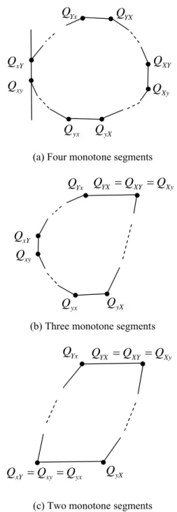
above variables, the first subscript denotes the extremum of coordinate and the second subscript denotes the extremum of the other coordinate under the first coordinate. Subscripts of capitalization and minuscule mean maximum and minimum, respectively, as shown in Fig.1. The definition of these points is given below. Definition 1.In the planar point set Q, Qxy, QxY, QXy, QXY,
Qyx, QyX ,QYx and QYX are the extreme points of the
convex hull, where Qxy and QxY, QXy,and QXY, Qyx and
QyX, QYxand QYX are the homogeneous extreme points,
respectively.
Theorem 1.The extreme points in the planar point set Q
are the convex hull vertices.
Proof. Assume that points q1, q2, , qMare convex hull
vertices, and make a line lparallel to y-axis through Qxy
and QxY. Suppose Qxy and QxY are not the convex hull
vertices, as shown in Fig.1 (a). According to their definition, points are all on lor on the right side of l. For
any vertex qi, if qiis on l, it must locate between Qxyand
QxY. This means that it can’t be a convex hull vertex. So
these vertices are all on the right side of l. Thus Qxyand
QxY fall in the left side of the convex hull instead of its
interior. This contradicts the convex hull definition. Therefore Qxyand QxYare vertices. Similar proofs can be
given to other extreme points.
(a) Four monotone segments
(b) Three monotone segments
(c) Two monotone segments
Figure 1: Extreme points and monotone segments of the convex hull
YX XY Xy
Q
Q
Q
Yx
Q
yX
Q
xY xy yx
Q
Q
Q
YX XY Xy
Q
Q
Q
yX
Q
Yx
Q
yx
Q
xY
Q
xy
Q
yx
Q
Q
yXXY
Q
Xy
Q
YX
Q
xY
Q
Yx
Q
xy
2.2
Convex hull monotonicity and its
construction
For segment QxYQYx of convex hull, let its points be
numbered in a clockwise order, namely qm, qm+1, …, qn (n
> m), where qi’s coordinate is (xi,yi), qm= QxY andqn=
QYx. Then qm, qm+1, …, qn-1should be on the same side of
straight line
q q
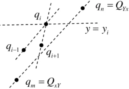
m n and the x-coordinate and y-coordinateof qm+1 should both increase. Suppose that both the x
-coordinates and y-coordinates of qm+1, qm+2, …, qi
monotone increase while those of qi+1decrease (either or
both of them decrease). Since qm,qi+1, qnare on the same
side of straight line
q q
i1 i, thus qi+1 should lie beneaththe line y=yi, as shown in Fig.2 (a). Hence qi-1 and qnare
on the different sides of the line
q q
i i1. This contradicts the fact that qm, qm+1, …, qn (n > m) are all the convexhull vertices. Therefore both the x-coordinates and y
-coordinates of points on segment QxYQYx monotone
increase. Similarly, the x-coordinates of points on
segment QYXQXY monotonically increase while the y
-coordinates of them decrease. The x-coordinates of
points on segment QyxQxymonotonically decrease while
the y-coordinates of them increase. Both two coordinates
of points on segment QXyQyX monotonically decrease.
The monotonicity of these segments is defined as follows.
Figure 2: Convex hull monotonicity
Definition 2. If QxY QYx, the convex hull segment
consisting of vertices from QxYto QYxis called monotone
increasing top segment. Likewise, if QYX QXY, the
convex hull segment consisting of vertices from QYX to
QXYis named monotone decreasing top segment. If QXy
QyX, the convex hull segment consisting of vertices from
QXy to QyX is called monotone decreasing bottom
segment. If QyxQxy, the convex hull segment consisting
of vertices from Qyxto Qxyis named monotone increasing
bottom segment.
Definition 3. All the monotone (both increasing and decreasing) top and bottom segments are called monotone segment.
If the monotone segments of a given convex hull are already determined, utilizing the definition 2 and the 8 extreme vertices can determine whether a specific monotone segment exists or not. The detailed theorem is as follow.
Theorem 2. The monotone increasing top segment exists if and only if QxY QYx. The monotone decreasing top
segment exists if and only if QYX QXY. The monotone
increasing bottom segment exists if and only if QXyQyX.
The monotone decreasing bottom segment exists if and only if QyxQxy.
Similarly, according to the definition of convex hull monotonicity, the type of monotone segments can be determined by its vertices. Let f(P, A, B) = 0 represent
the line equation, where the line runs through points A
and B, P is a dynamic point on the line. There is a
theorem about the type of monotone segments as follows. Theorem 3. Let qm, qm+1, …, qn (n - m > 1) be the
vertices on a specific monotone segment of convex hull, and the coordinate of qibe (xi,yi). For arbitrary i, j(m≤
i< j, m ≤ j < n, j i, j i + 1), the sufficient and
necessary conditions for that this monotone segment is a monotone increasing top segment are that
1 1)
0
,
,
f(
i i i i jy
y
q
q
q
. Likewise, as for the monotone
decreasing top segment, the monotone decreasing bottom segment, monotone increasing bottom segment, their sufficient and necessary conditions are
1 1)
0
,
,
f(
i i i i jy
y
q
q
q
,
1 1)
0
,
,
f(
i i i i jy
y
q
q
q
,
1 1)
0
,
,
f(
i i i i jy
y
q
q
q
, respectively.According to the convex hull definition, it has 4 monotone segments at most. Since convex hull is a closed shape, it has two monotone segments at least. The number of monotone segments can be determined by the extreme points. According to the number of monotone segments, convex hulls are classified into three types, as shown in Fig.1. Fig.1 (a) shows the convex hull with 4 monotone segments, Fig.1 (b) and Fig.1 (c) show the convex hull with 3 and 2 monotone segments, respectively.
3
Convex hull algorithm for binary
image
3.1
Algorithm of monotone segment
Since the extreme points are convex hull vertices, the convex hull can be obtained by determining the vertices on the monotone segments between each pair of extreme points. In this work, a dynamic computation method is applied to determine the convex hull. Calculate the extreme points and determine the monotone segments. By dynamic scanning the boundary of image, the temporal convex hull of the scanned image is obtained. Scan the image boundary pixel by pixel until encountering the last boundary pixel. Thus, the monotone segments are obtained and the convex hull is extracted. The theorem of convex hull computation is as follows. i
y
y
1 i
q
iq
1 iq
n Yxq
Q
m xY
Theorem 4. Let Q = {qm, qm+1, …, qn} (n > m) be the
vertices of a monotone segment of a specific convex hull, the coordinate of qi and p be (xi, yi) and (x, y),
respectively, Q = {p}Q and min{yn1,yn} < y <
max{yn1,yn}. If pand qk(k<n) are both the points in a
specific monotone segment of Q, then qm, qm+1, …,qk,p,
qnare all vertices on the monotone segment.
Proof: Suppose that qm, qm+1, …, qn (n > m) are the
vertices of monotone increasing top segment of a specific convex hull. Since p(x, y) belonging to {p}Qis a point
on the monotone increasing top segment and yn1< y<
yn, then f(p, qn1, qn) > 0 according to theorem 3. The
location of pis shown in Fig.4. If qk(k<n) belonging to
{p}Q is a vertex with maximum subscript on the
monotone increasing top segment, then qk and p are
adjacent vertices on the new monotone increasing top segment. So for all qi(ik), f(p, qn1, qn)<0. If qj(j < k)
isn’t the vertex of new convex hull, then f(p, qj-1, qj)>0.
But f(qk, qj1, qj)<0. It means that qk and p are on the
different side of line
q
j1q
j. So f(qk, p, qj)<0. Thereforeqk isn’t the vertex of new convex hull. This contradicts
the precondition. Hence qm, qm+1, …, qk, p,qnare vertices
on the monotone segment. Likewise, similar proofs of other monotone segments can be easily given.
Figure 3: Monotone algorithm
Whether or not a pixel or a boundary point is a convex hull vertex depends on the relation about its position and the line. Take the monotone increasing top segmentqm, qm+1, …, qn(n>m) for example. Theorem 3
shows that f(qj, qi, qi+1) < 0 for arbitraryi, j(m≤i<j,m ≤j <n,j i,j i+ 1). If a point pof image boundary
satisfies f(p, qn-1, qn) > 0, then p is outside of the
temporary convex hull. Thus pmust be a new vertex of
convex hull. Start fromk=n1 and decrease kby 1 each
time. If f(p, qk, qk1) < 0, then for arbitrary point A(A
qk1, Aqk), f(A, qk, qk1) < 0. According to theorem 3,
qkis a new vertex of convex hull. By applying theorem 4,
all vertices on this segment can be obtained.
3.2
Convex hull algorithm for binary
image
Convex hull of binary image can be determined by its boundary pixel set. In fact, the convex hull of boundary pixel set is equal to the convex hull of binary
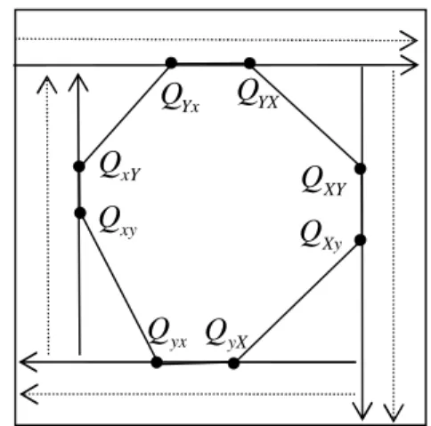
image. So obtaining the boundary is an important step. Generally, boundary extraction by scanning the whole image requires storing all pixels. However, only few pixels are the convex hull vertices. Reducing the number of scanned pixels can both improve the time and space efficiency of algorithm. In this section, the method scanning from outside to inner is applied to extract the extreme points, as shown in Fig.4. The scanned regions are determined by the extreme points. By dynamic scanning the image boundary, temporary convex hull of the scanned boundary pixel set is computed. Finally, convex hull of binary image is available.
Figure 4: Extreme points of image convex hull
3.2.1 Collect the extreme points
In order to avoid repeated scanning, the method scanning from outside to inner is utilized to collect the extreme points on the image boundary. The detailed steps are as follows.
STEP 1: Begin at the top left of image and scan image from top to bottom until encountering the image boundary. Each row scan starts from left to right. If the scanned row has boundary points, QYx and QYX represent
the leftmost and rightmost boundary points, respectively. Thus two extreme points on the image boundary, QYx and
QYX, are obtained.
STEP 2:Begin at the line l1running through QYx and
QYX and scan image from right to left until encountering
the image boundary. Each column scan starts from top to bottom. For the column having boundary pixels, let QXY
and QXy represent the topmost and bottommost boundary
pixels, respectively. Thus two extreme points on the image boundary, QXYand QXy, are obtained.
STEP 3:Begin at the line l2running through QXY and
QXy and scan image from bottom to top until
encountering the image boundary. Each row scan starts from right to left. For the row having boundary pixels, let
QyX and Qyx represent the rightmost and leftmost
boundary pixels, respectively. Thus two extreme points on the image boundary, QyXand Qyx, are obtained.
STEP 4: Start from the line l3 which is through Qyx
and QyX to the line l1 and scan image from left to right
until encountering the image boundary. Each column scan starts from bottom to top. For the column having boundary points, let QxY and Qxy represent the topmost
Yx
Q
Q
YXxY
Q
xy
Q
yX
Q
yx
Q
Xy
Q
XY
Q
m
q
n
q
j
q
1
n
q
k
q
1
j
q
and bottommost boundary pixels, respectively. Thus two extreme points on the image boundary, QxYand Qxy, are
obtained.
By the above steps, 8 extreme points of image convex hull are extracted.
3.2.2 Determine the scanned regions
Theorem 1 shows that the 8 extreme points are convex hull vertices. The lines connecting adjacent extreme points divide image into several regions, as shown in Fig.5. There are no boundary pixels outside of the rectangle formed by l1, l2, l3 and l4. If the boundary pixels are on the edges of the rectangle, then they aren’t convex hull vertices. In the interior of the rectangle, pixels in region 0 aren’t vertices either. Only those in regions 1, 2, 3 and 4 are likely to be vertices. Hence we just need to scan region 1~4 to obtain the boundary pixels and compute the convex hull by applying theorem 4. Since the vertices are numbered in a clockwise order, pixels extracted by scanning the four regions should satisfy theorem 4. The detailed method is as follows.
Figure 5: Scanned regions of image
Region 1:Begin at the right side ofl4and scan the region
1 horizontally from left to right. Each column in region 1 is scanned vertically from top to bottom. If there is no boundary pixel on the scanned line, then scan next column until encountering a boundary point p on the
scanned line. Then pis a vertex of temporary convex hull
in the scanned image. Compute the monotone increasing top segment of temporary convex hull by theorem 4. To improve the efficiency of algorithm and guarantee that the next scanned boundary pixels must be the vertices of temporary convex hull, the next column scan should stop once reaching the line pQYx, as shown in Fig.6 (a).
Continue to scan and compute the vertices of temporary convex hull until QYx is encountered.
Region 2: Begin at the down side of l1and scan region 2
vertically from top to bottom. Each row in region 2 is scanned from right to left. Utilize the similar method introduced in region 1 to determine whether the boundary pixels are vertices or not. Continue to scan until QXY is
encountered, as shown in Fig.6 (b).
Region 3: Begin at the left side of l2and scan region 3
horizontally from right to left. Each column in region 3 is scanned from bottom to top. Utilize the similar method introduced in region 1 to determine whether the boundary pixels are vertices or not. Continue to scan until QyX is
encountered, as shown in Fig.6 (c).
Region 4: Begin at the left side of l3and scan region 4
vertically from bottom to top. Each row in region 4 is scanned from left to right. Utilize the similar method introduced in region 1 to determine whether the boundary pixels are vertices or not. Continue to scan until Qyxis encountered, as shown in Fig.6 (d).
The extracted boundary pixels in the above steps both satisfy the monotone condition and the sequence required by theorem 4. Applying theorem 4 can extract the convex hull of image.
(a) Scan in region 1
(b) Scan in region 2 xY
Q
xy
Q
Q
XYXy
Q
YX
Q
Yx
Q
yX
Q
yx
Q
XY
Q
Xy
Q
YX
Q
Yx
Q
yX
Q
pyx
Q
0 1
2
3 4
l1
l2
l3
l4
QYX
QYx
Qxy
QxY
QyX
Qyx
QXy
QXY
xY
Q
xy
(c) Scan in region 3
(d) Scan in region 4
Figure 6: Scanned areas in each region
3.2.3 Compute convex hull vertices in
scanned areas
Whether or not the pixel in scanned area is a convex hull vertex is just relative to other pixels in this region. By scanning the boundary pixels in each region, convex hull vertices in the corresponding region can be determined, respectively. Take region 1 for example. Let (xm1, ym1) and (xm2, ym2) be the coordinates of QxY and
QYx, respectively, f(p, A,B) = 0 be the equation of line
running through Aand B (p is a dynamic point), v[i][j]
and c[i][j] be the pixel value and coordinate of p in the ith row and the jth column of the image, respectively. If v[i][j] > 0, p is a boundary pixel, or less a background
pixel. Begin at (xm1 + 1, ym1 + 1) and scan region 1
horizontally from left to right. In region 1, column is scanned from top to bottom. If there is no boundary pixel in the current column, scan next column in its right. If pixel p is a boundary pixel, then it must be a vertex of
temporary convex hull. Apply theorem 4 to compute all vertices of temporary convex hull. Scan next column in the right. At this time, the scanned line is above the line
pQYx, as shown in Fig.6 (a). Stop scanning when the line
x = xm2is encountered. Then the monotone segment of
convex hull in region 1 is extracted. The detailed algorithm is as follows.
STEP 1: i=xm1+1, j=ym2-1, q1= QxY,A=QxY, n=2;
STEP 2:IF (i xm2) goto STEP 8;
//no boundary pixel on the scanned line IF (f(p, A,QYx)0) goto STEP 3;
//pis a vertex of temporary convex hull
IF (v[i][j] > 0) //pis the foreground pixel. k=n1, A=c[i][j], goto STEP4; ELSE goto STEP5; //scan next pixel STEP 3: i=i+1, j=ym2-1, goto STEP 2;
//scan next vertical line in the right STEP 4:IF (k>1) goto STEP 6;
ELSE n=n+1,goto STEP 2; STEP 5: j=j+ 1, goto STEP 2;
STEP 6:IF (f(p,qk1,qk)0) // backtrack again.
goto STEP 7;
ELSE // finish backtracking
n=k+1, qn=c[i][j], n=n+1, goto STEP
2;
STEP 7:IF (k>2) //backtrack and process next pixel k=k1, goto STEP 6;
ELSE //backtrack to the extreme point
n= 2, qn=c[i][j], n=n+ 1, goto STEP 2;
STEP 8: qn=QYx,q1,q2,…,qnare convex hull vertices.
3.2.4 Convex hull algorithm for binary
image
For the convex hull of binary image, compute the 8 extreme points Qxy, QxY, QXy, QXY, Qyx, QyX, QYxand QYX.
According to these extreme points, determine the scanned regions of image, as shown in Fig.5. Then, convex hull vertices locate the regions 1~4, which are divided by the lines connecting the adjacent extreme points, as shown in Fig.5. Therefore, only the boundary pixels in these regions require computation. Utilize the monotone properties of convex hull and scan each region dynamically. Then, apply theorem 4 to compute each monotone segment of convex hull. The entire convex hull is obtained by merging these monotone segments. The detailed algorithm is as follows.
STEP 1: Scan the binary image and compute the 8 extreme points,Qxy, QxY, QXy, QXY, Qyx, QyX, QYxand QYX.
STEP 2: Utilize the 8 extreme points to determine the four regions where the convex hull vertices may exist. STEP 3: Scan each region dynamically and obtain convex hull vertices on each monotone segment respectively.
STEP 4: Extract convex hull vertices on each monotone segment according to the following order,
QxYQYx, QYXQXY, QXyQyX, QyxQxy. Each extreme
point is extracted only one time. Then convex hull is obtained.
4
Complexity analysis
4.1
Time complexity
The time complexity is analyzed in the following ways. Suppose that the size of binary image is NN.
(1) If the image consists of a single pixel, then no convex hull exists. The time complexity is N2.
xY
Q
xy
Q
Q
XYXy
Q
YX
Q
Yx
Q
yX
Q
yx
Q
XY
Q
Xy
Q
YX
Q
Yx
Q
yX
Q
yx
Q
xY
Q
xy
(2) If the image consists of two pixels or all pixels are on a line, then no convex hull exists, either. The time complexity is alsoN2.
(3) The binary image has a convex hull if and only if three boundary pixels at least aren’t on a line. Suppose that there are Spixels in the polygon whose vertices are
the adjacent and inhomogeneous extreme points. The proposed method scansN2S pixels at most.And only
2N pixels at most should be computed when it
determines whether or not a boundary pixel is a convex vertex. So the time complexity is O(N2S) +O(N).
The above analyses show that the bigger the convex hull of binary image, the less the time complexity of the proposed algorithm. The time complexity of convex hull algorithm mainly depends on the size of scanned area. To show the efficiency of time complexity, we compare the proposed algorithm with the algorithm presented in [17]. A typical example is given in Fig.7. Fig.7 (a) is a binary image containing an object whose boundary has 10 vertices. Both algorithms are exploited to extract convex hull of the object in the binary image. Fig.7 (b) and Fig.7 (c) show the scanned areas of the algorithm [17] and the proposed algorithm respectively, where the gray grids denote their scanned areas. It is observed that our algorithm scans less area than the algorithm [17]. In general, if the object’s boundary isn’t a convex polygon, the scanned areas of the proposed algorithm are less than those of the algorithm [17]. Otherwise, the scanned areas of two algorithms are equivalent. Hence, the proposed algorithm needs less time than the algorithm [17] on average.
(a) Binary image containing an object with 10 vertices
(b) Scanned areas of the algorithm [17]
(c) Scanned areas of the proposed algorithm Figure 7: A binary image and its scanned areas using
different algorithms
4.2
Space complexity
The boundary pixels scanned by the proposed algorithm are the vertices of temporary convex hull. During the convex hull computation, only these vertices require storage. Therefore, the proposed algorithm has a low space complexity. Take Fig.7 for example. The algorithm [17] must store all 10 points from p0 to p9.
Since p2 and p6 aren’t scanned, the proposed algorithm
doesn’t need to compute and store them. So the space complexity of the proposed algorithm is lower than that of the algorithm [17].
5
Conclusions
In this paper, we derive some new convex hull properties, such as monotonicity, and use them to design algorithm for extracting convex hull of object in binary image. The proposed algorithm has a high efficiency by reducing computational cost in the following ways. (1) Divide the binary image into several regions by using the extreme points. Only those boundary pixels in a few regions require computation. (2) To determine a vertex in a given region doesn’t need to compute those pixels in other regions. (3) Since the boundary pixels obtained by
p0
p1
p2
p3
p4
p5
p6
p7
p9
p8
p0
p1
p2
p3
p4
p5
p6
p7
p8
p9
p0
p1
p2
p3
p4
p5
p6
p7
p8
scanning are computed dynamically, only these vertices of temporary convex hull require storage. Theoretical analyses show that the proposed algorithm has lower complexities of time and space than the algorithm [17] on average.
Acknowledgement
This work was partially supported by the Natural Science Foundation of China (60963008, 60763011), the Natural Science Foundation of Guangxi (0832104, 0447035), the project of the education administration of Guangxi (200911MS55, 200607MS135), and the Scientific and Technological Research Projects of Chongqing’s Education Commission (KJ081309). The authors would like to thank the anonymous referees for their valuable comments and suggestions.
References
[1] Bhaniramka P., Wenger, R., and Crawfis, R. (2004) Isosurface construction in any dimension using convex hulls. IEEE Transactions on Visualization and Computer Graphics, vol.10, no.2, pp.130–141.
[2] Yuan B., and Tan C. L. (2007). Convex hull based skew estimation. Pattern Recognition, vol.40, no.2,
pp.456-475.
[3] Nikolay M. Sirakov et al. (2004). Search space partitioning using convex hull and concavity features for fast medical image retrieval. In: Proc. of the IEEE International Symposium on Biomedical Imaging, Arlington, USA, pp.796–799.
[4] Yu X., Sun H., and Chen J. (2005). Points matching via iterative convex hull vertices paring. in: Proc.of the fourth International Conference on Machine Learning and Cybernetics, Guangzhou, China, pp.
5350–5354.
[5] Gope C., and Kehtarnavaz N. (2007). Affine invariant comparison of point-sets using convex hulls and hausdorff distances. Pattern Recognition,
vol.40, no.1, pp.309–320.
[6] Yu M. P., and Lo K. C. (2001). Object recognition by combining viewpoint invariant Fourier descriptor and convex hull. in: Proc. of the 2001 International Symposium on Intelligent Multimedia, Video and Speech Processing, Hong Kong, China,
pp.401–404.
[7] Chand D. R., and Kapur S. S. (1970). An algorithm for convex polytopes. JACM, vol.17, no.1, pp.78–
86.
[8] Jarvis R. A. (1973). On the identification of the convex hull of a finite set of points in the plane.
Information Processing Letters, vol.2, no.1, pp.18–
21.
[9] Graham R. L. (1972). An efficient algorithm for determine the convex hull of a finite linear set.
Information Processing Letters, vol.1, no.1,
pp.132–133.
[10] Preparata F. P. and Hong S. J. (1977). Convex hulls of finite sets of points in two and three dimensions.
CACM, vol.20, no.2, pp.87–93.
[11] Chan T. (1996). Optimal output-sensitive convex hull algorithms in two and three dimensions.
Discrete Comput. Geom, vol.16, no.3, pp.361–368.
[12] Chen W., Wada K., and Kawaguchi K. (2002). Robust algorithms for constructing strongly convex hulls in parallel. Theoretical Computer Science,
vol.289, no.1, pp. 277–295.
[13] Brönnimann H. et al. (2004). Space-efficient planar convex hull algorithms. Theoretical Computer Science, vol.321, no.1, pp.25–40.
[14] Overmars M. H., and Leeuwen J. V. (1981). Maintenance of configurations in the plane. J. Comput. System Sci., vol.23, no.2, pp.166–204.
[15] Chan T. M. (2001). Dynamic planar convex hull operations in near-logarithmic amortized time.
Journal of the ACM, vol.48, no.1, pp.1–12.
[16] Brodal, G. S., and Jacob R. (2002). Dynamic planar convex hull. in: Proc. of the 43rd Annual IEEE Symposium on Foundations of Computer Science,
Vancouver, Canada, pp.617–626.