A Proposal to Expand the Community
of Users Able to Process Historical
Rainfall Data by Means of the Today
Available Open Source Libraries
Paolino Di Felice
1, Luca Finocchio
2, Daniele Leombruni
2and
Vittoriano Muttillo
21Department of Ingegneria Industriale e dell’Informazione ed Economia, University of L’Aquila, Italy 2Master students in Engineering Informatics, University of L’Aquila, Italy
The paper presents a software architecture based on open source technologies, implemented by the authors in an experience of processing spatio-temporal data gathered by rain gauges spread across two regions of central Italy. The interest in the automatic processing of data about precipitation is widespread, however, today only an inner circle of stakeholders can think of taking advantage of the available open source libraries because a strong programming skill is required to use them. It is opinion of the authors that the implemented software architecture is suitable for expanding the community of users able to process “by themselves” historical precipitation data. The centre of the architecture is the technology of the spatial database management systems. They offer full support for the creation and management of a spatial database suitable to store the rainfall data usually spread out in several files. Moreover, they allow adding to such a repository a large set of ad hoc “objects” oriented to carrying out spatio-temporal computations on the precip-itation. The stakeholders are only required to familiarize with the database’s objects and invoke their execution. A large part of the paper is devoted to show how the adopted conceptual setting can assist nontechnical users in carrying out personalized computations on rain gauges data. The computing needs posed by the experience described in this paper are common to many other areas of high social impact that involve spatio-temporal data, hence we believe that the implemented framework can be exported to them, keeping unaltered operational effectiveness.
Keywords: open source software, DBMS, SQL, Post-GIS, R language, software architecture, user defined function, precipitation retrieval
1. Introduction
The wise management of water reserves, the prevention of natural disasters related to ex-cessive rains, and the choise of the best land use in agriculture are few issues of primary im-portance to most countries. The modeling of these scenarios and the efficient management of the huge amount of spatio-temporal data in-volved are very complex problems that must be addressed with methods and tools from the ar-eas of computing and information technology. Some of the recent contributions in this direc-tion are: (Lu and Wong, 2008; Krishnakumar et al., 2009; Li et al., 2011; Rowhania et al., 2011; Tabari and Talaee, 2011; Ahani et al., 2012; Bostan et al., 2012; Keblouti et al., 2012; Chen and Liu, 2012).
individual spreadsheet files. Spreadsheets also make it difficult to analyze data categorically, such as on a daily or monthly time step.” To overcome this limit, the software architecture we present in this paper, and implemented in a recent experience of storage, cleaning, process-ing and visualization of spatio-temporal data collected by rain gauges located on two regions of central Italy, puts at the centre the technol-ogy of the Spatial Database Management Sys-tems(SDBMSs). This technology has dramati-cally increased the effectivness and efficiency in carrying out many everyday activties involving large structured datasets.
Our software architecture is based exclusively on open source technologies. Since several years ago there has been a consolidation of open source software able to manipulate spatio-temporal data. This fact, together with the appearance of international no-profit founda-tions (e.g., Open Source Geospatial Founda-tion – OSGeo), indicates that the interest in open source software is expected to grow sig-nificantly in the near future. Steiniger and Bocher(2009)recognize four indicators of this trend: (1)increasing number of projects run us-ing open source GISs, (2)increasing financial support by government agencies, (3) increas-ing download rates, and(4)increasing number of use-cases. With regard to the geostatistical computations of rainfall data, in particular, the use of the R environment(Pebesma, 2004), ex-tended with libraries such as gstat and raster, today appears as the best choice. Unfortunately, as stressed by Hengl (2009) – page 90, “the main problem with R is that each step must be run via a command line, which means that the analyst must really be an R expert”. This circumstance limits the use of this valuable soft-ware tool to subjects with strong programming aptitude.
Thanks to the possibility of formulating “pow-erful” spatial queries at a “high level” of ab-straction, SDBMSs have the further merit of greatly extending the community of those who can interact with such a software technology to perform relevant spatial analysis without own-ing a specific IT skill. In the experience of computing of spatio-temporal data reported in this paper, the queryexpressivenessis obtained by placing side by side to the basic SQL opera-tors and to the built-in functions of the SDBMS, “database objects” created ad hoc(technically
they are User Defined Functions – UDFs), while the abstraction is obtained by masking to the end user the logical structure of the underlying database(for example, through the mechanism of the views), as well as the functions called in the query. From the stakeholders involved is only required to familiarize with the objects that the database exposes and invoke their execution. This level of competence can be achieved after a short on-the-job training of the nontechnical personal.
The paper is divided in two parts. The first part: a) proposes the technological solution setting and lists its several advantages over the current ways of processing historical data about precip-itation (Section 2), b) describes the reference format of the rainfall data, the design of a Spa-tial DataBase(SDB)adequate to store the data about the geographical area of interest, the rain gauges spread over it, and the collected mea-surements (Section 3), c) gives details about the structuring of a number of packages that im-plement the computing requirements posed by the application domain we refer to(Section 4), and, finally, d)discusses the related work( Sec-tion 5). The second part of the paper(Section 6)
shows, through a case study about rainfall data recorded by rain gauges located in central Italy, the simplicity with which, working from the in-side the console of the SDBMS, one could take advantage of the many features offered by the packages we have developed(and displayed as database objects)to implement the phases rang-ing from the storage of the measurements in the SDB, to their cleaning and processing, till the production of maps.
2. The Solution Setting
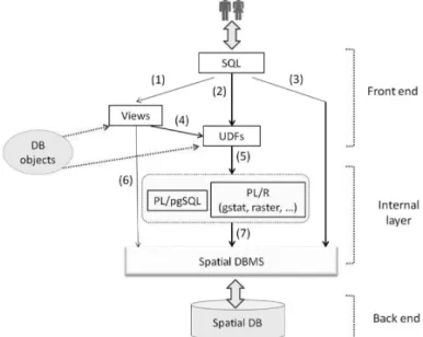
Figure 1 shows the reference software architec-ture of our solution setting. It can be interpreted at two different levels: oneabstract, the other
The central element of the architecture of Fig-ure 1 is the technology of the SDBMSs. It offers enormous advantages over the current ways of processing the historical data about precipita-tion; in detail, it allows us:
Figure 1.The reference software architecture.
1. to keep together, in a single container, all the historical measurements. Data typically dis-persed in a multitude of independent files, sometimes conflicting even in their format; 2. to limit the access to the data only to people
holding explicit granting privileges;
3. to call the spatial operators of the SQL lan-guage as well as the spatial built-in UDFs, when querying the SDB. UDFs are a rel-evant capability of SDBMSs. For exam-ple, PostgreSQL/PostGIS (ver. 9.2, Pos-GIS model: postgis 21 sample)offers 1092 built-in UDFs;
4. to code ad hoc views and UDFs (to be added to the built-in UDFs) to be exposed as database objects, both joinable in SQL queries of extraordinary expressiveness; 5. to transform the end users’ rainfall data
pro-cessing needs from programming activities, as it happens today, to querying activities against the SDB, with considerable masking of technicalities and, therefore, potentially widening the number of those who in the fu-ture could face such difficulties with profit. In fact, by taking advantage of the geosta-tistical and graphical functionalities of the R programming environment (and of the li-braries linked to it, over allgstatandraster),
with which the SDBMS communicates ef-fectively, it is easy to greatly extend the ca-pabilities of the SQL-pure UDFs(i.e., func-tions written by embedding SQL commands into the internal language of the SDBMS), greatly simplifying the job of the end users. Figure 1 shows the paths through which users can interact with the SDB. In each path, it is required to write SQL queries to be executed in the console of the SDBMS. For users without any technical skill, the interaction with the rain-fall data takes place by invoking the database objects (either path 1 or 2), while path (3) is for skilled users. Path(1)may involve objects of type view (path 1-6), or views and UDFs together(path 1-4-5-7), while path(2-5-7) in-volves only UDFs. If the user invokes in the query some UDFs, he/she, however, does not perceive their internal encoding, and even the coding language(either PL/pgSQL or PL/R). To learn about the merits of the R environment, refer to(Hengl, 2009). The literature already proposes examples of usage of R to develop packages(e.g., Cannon, 2011).
The communication between PostgreSQL and R may take place either by keeping them sep-arate, or by using R from inside PostgreSQL. Choosing the first option, they communicate by importing/exporting shapefiles: so, one can, for example, run a query in PostgreSQL, export the result as a shape, load it into R and, eventu-ally run(in this environment)the processing he is interested in. But because, as already men-tioned, work with R implies that the analyst must really be an R expert, we decided to adopt the second option in which the use of R is hid-den to the end users of the SDB, therefore, they may not be programmers.
PostgreSQL allows us to interact with the R environment by using PL/R, i.e., a procedural language suitable for writing PostgreSQL func-tions in the programming language R. PL/R provides most of the R’s functionalities.
3. Format of the Precipitation Data and Structure of the Spatial Database
data format. Burnette and Stahle (2013) re-port a similar situation for the United States. In this paper, we will refer to the data format adopted by the Italian Department of Civil Pro-tection, which is a structure of the Presidency of the Council of the Ministers( http://www.pro-tezionecivile.gov.it). Section 6.1 explains how our packages intercept the format hetero-geneity in case the precipitation data come from a different source, allowing, therefore, to keep the structure of the SDB unaltered.
3.1. Format of the Precipitation Data
The rainfall data are collected in two categories of files. The first one consists of a single file about the stations of measures distributed over the land, while the second category is composed of many files as the months to which the mea-surements refer to. The rain gauges measure the precipitation volume(in mm)each 15 min-utes using a counter that is incremented by one each time it detects 0.1 mm of rain. The rain gauge calculates the precipitation accumulated in the last quarter of an hour by subtracting from the current value of the counter the value of the counter at the previous measurement, and di-viding the result by 10(to express the value in mm).
The metadata about the rain gauges are de-scribed by the tuple: <id, name, station num-ber, municipality, region, geographical posi-tion> the latter expressed as latitude and longi-tude. The metadata about the rainfall measure-ments are described by the tuple: <rain gauge id, data, hour, rainfall in 15 minutes (mm),
counter>.
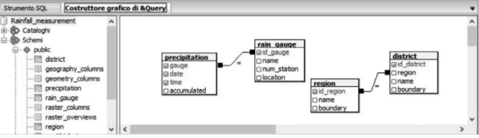
3.2. Structure of the SDB
The SDB(calledRainfall measurement) suit-able to hold the data of interest is composed of the four tables of Figure 2. region and dis-trictrefer, respectively, to the region and the municipality where the meteorological stations are located.
The SQL/DDL statements about the four tables of Figure 2 are given in the Appendix.
4. Organization of the Packages
The precipitation context raises many process-ing requirements. We discuss them in the fol-lowing. The initial need consists of loading the measurements recorded by the rain gauges into the SDB. Subsequently, it is useful to perform an analysis about the distribution of the stations over the land. In fact, the sampling density plays a significant role in the performance of the spatial interpolation methods. Li and Heap
(2008)report that “when data are sparse, the un-derlying assumptions about the variation among samples may differ and the choice of a spatial interpolation method and parameters may be-come critical.”
The validation of the data about the precipita-tion is another crucial issue for increasing their quality. Data quality is among the major factors that affect the performance of the spatial inter-polation methods (Li and Heap, 2008). Data noise can negatively affect the output of those methods.
The construction of diagrams about the trend of the rainfall for time intervals selected on an hourly, daily, weekly, monthly or yearly basis is another crucial requirement.
Interpolation of the measured data over the geo-graphical area with the ultimate goal of getting maps about the rainfall is fundamental. Inter-polation techniques widely used are the inverse distance interpolation (IDW) method and the Kriging(Li and Heap, 2008). The cross valida-tion of the interpolavalida-tion carried out is mandatory to evaluate the results.
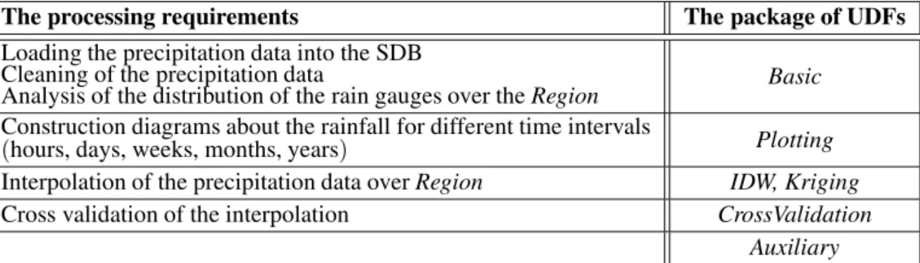
Table 1 brings together the processing require-ments and the name of the corresponding pack-age of PostgreSQL UDFs that implements them. The Auxiliary package contains 34 functions created to support those contained in the other
five packages. Table 2 lists the 34 functions di-vided according to the used coding language
(namely: PL/R or PL/pgSQL). The names of these functions are left intentionally generic
(UDF 0, UDF 1,...) so as not to create confu-sion or conflict with the name of the functions that invoke them.
Table 3 shows, for each package, the number of internal UDFs, the total number of lines of code, the number of UDFs of the packageAuxiliary
called. From Table 3 we learn about the mas-sive use that the UDFs of the various packages make of the UDFs of theAuxiliarypackage. The PL/pgSQL code refers to version 9.2 of PostgreSQL and to version 1.8 of PostGIS, while the PL/R code refers to version 8.3.0.14.
The processing requirements The package of UDFs
Loading the precipitation data into the SDB Cleaning of the precipitation data
Analysis of the distribution of the rain gauges over theRegion Basic Construction diagrams about the rainfall for different time intervals
(hours, days, weeks, months, years) Plotting
Interpolation of the precipitation data overRegion IDW, Kriging Cross validation of the interpolation CrossValidation
Auxiliary
Table 1.The processing requirements.Regiondenotes a generic geographic area.
Language Name of the UDF
PL/R UDF 0, UDF 6, ..., UDF 14,UDF 16, ..., UDF 23, UDF 27, ..., UDF 31 PL/pgSQL UDF 1, ..., UDF 5, UDF 15, UDF 24, UDF 25, UDF 26, UDF 32, UDF 33, UDF 34
Table 2.List of the UDFs in theAuxiliarypackage.
Package Total # of UDFs Total # of lines of code package Auxiliary calledTotal # UDFs of the
Basic 7 205 1
Plotting 20 604 36
IDW 4 206 (4∗4=)16
Kriging 16 760 (16∗4=)64
CrossValidation 12 421 (12∗2=)24
Auxiliary 34 1026
5. Related Work
(Ward et al., 1996), a pioneering work in the field of geocomputing, outline a computational architecture suitable to deal with the complexity and the diversity of data and processing needs in geoscientific data analysis. One of the key el-ements of the proposed architecture is the layer about the management of data. The architec-ture we implemented to carry out the experi-ence about spatio-temporal raing gauges data intercepts this recommendation.
In (Shen et al., 2005), a relational database is introduced as the backbone of a system to deal with hydrological data.” Authors attribute three major merits to their system’s underly-ing database-supportunderly-ing architecture: a)“great flexibility for user manipulation and customiza-tion”; b) “the great potentiality deriving from using the built-in database functions”; c) “the database builds a linkage among users’ inputs, model data management, and the numerical model by implementing a set of dynamic database queries.” The above three merits apply to our solution as well.
In the same year, (Carleton et al., 2005) de-veloped a Microsoft Access database designed to facilitate the storage, retrieval and analysis of hydrologic data as an alternative to the prevalent trend at the time of storing such data in spread-sheets which, as already pointed out, suffer from severe limits. Besides presenting the database structure, (Carleton et al., 2005) provide a set of queries useful to retrieve data that involve calculations, comparisons and basic quality as-surance/quality control calculations. Our ex-perience reaffirms the relevance of querying, besides showing a way to deeply enhance its expressiveness by calling ad hoc UDFs and/or views.
Pokorny (2006) remarks that since the 1960s there is an ever increasing environmental de-mand from customers, authorities and govern-mental organizations. Then, he states that “A natural idea is that environmental information systems based on advanced database technolo-gies could help to deal with these issues.” Our practical experience builds on both the above statements.
6. The Case Study
This section shows the ease of use, as well as the effectiveness, of the UDFs collected in the six packages developed (Table 3), to support the archiving, cleaning and processing of pre-cipitation data up to the production of rainfall maps. The discussion will involve only some of the UDFs.
The case study takes into account the measure-ments recorded in November 2007 by 137 mete-orological stations, equipped with a rain gauge, located in the regions of Lazio and Umbria( cen-tral Italy). The dataset about the rain gauges and that about the measurements are in the.csv format and follow the pattern described in Sec-tion 3.
6.1. SDB Loading
Preliminarily, the.csvfile about the rain gauges and the file about the measurements were both converted(by means of QGIS)into shape files. The shape files containing the geometry of the Italian regions and municipalities were down-loaded from ISTAT ( http://www.is-tat.it/). The format of the geometric data in all the shape files was expressed in the WGS 84 Spatial Reference System. Then, we imported
(using the appropriate pgAdminIII plug-in)the content of the shape files about the rain gauges, regions and municipalities inside, respectively, tablesrain gauge,regionanddistrictof the SDBRainfall measurement. The manual ac-tions mentioned so far are part of what we might callphase zero. From here on out, all the actions that will be described are greatly facilitated by the use of the UDFs developed.
To load the contents of the file of the measure-ments in the tableprecipitation is sufficient to invoke the UDF import precipitation() of the package Basic (written in pure SQL –
Appendix) which, in turn, engages the UDF 0
is obtained by running(in the query window of pgAdminIII)the SQL command:
SELECT import precipitation(‘...\ 2007-11csv’, ‘2007-11’)
This command must be invoked as many times as the months of the measurements to be loaded into the SDB(Section 3).
The invocation of any one of our UDFs has to be made in the same operating mode. In the following we will avoid repeating it.
6.2. Assessment of the Spatial Distribution of the Rainfall Stations Over
the Territory
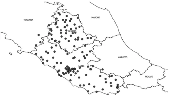
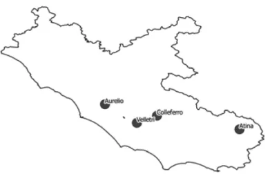
Figure 3 shows that spatial distribution of the 137 meteorological stations is not uniform; in particular, in the case of the Lazio region, there is a high density of rainfall stations around Rome. In Lazio (17,236 km2) there are 84 stations, in Umbria(8,456 km2)47.
Each dot represents one station. Some sta-tions are located slightly outside the two regions
(3 in Tuscany, 2 in Abruzzo and 1 in Campa-nia). A confirmation of what appears visually can be obtained by running the query SELECT count(*) FROM rainGauges filter(’LAZIO’), where rainGauges filter() is a UDF of the packageBasic.
As already mentioned(Section 4), the number of the meteorological stations and their distri-bution over the land impact the performance of
the spatial interpolation methods(Li and Heap, 2008). Table 4 shows that each rain gauge in Lazio covers, on the average, about 205 km2
while in Umbria it covers about 180 km2. These
data confirm that the number of rain gauges in Umbria is more appropriate than that in Lazio. In both cases, the numbers confirm a trend well known in the literature, namely that frequently the number of stations is very low when com-pared to the size of the territory. For example, Bostan et al. (2012) report on a study about the annual precipitation in Turkey carried out by starting from the measurements acquired in just 225 meteorological stations throughout the entire country(an area of 783.562 km2).
There-fore, it is legitimate to conclude that the situation in Lazio and Umbria is definitely more favor-able.
Region Rain gauges distribution(km2)
Lazio 204.7
Umbria 179.8
Table 4.Distribution of the rain gauges in Lazio and Umbria. These values are computed by running the
(Basic)UDFrainGauges density().
6.3. Data Cleaning
Using the (Basic) UDFs clean peaks() and clean gauge()(to be invoked as: SELECT cle-an peaks(3); SELECT clean gauge(3,30))it is
possible to eliminate the outliers and the suspi-cious rain gauges as well. Specifically, the first query eliminates from tableprecipitationall the tuples that in the fieldaccumulated have a value of the rainfall in 15 minutes greater than 3 mm, while the second query eliminates from table rain gaugethe corresponding stations if it happens that they have a percentage of er-roneous readings above 30%. The arbitrarily set threshold value of 3 mm in 15 minutes of precipitation can be adjusted to the geographic region of reference.
6.4. Measurements Plotting
Diagrammatic visualization of the measurements collected in the SDB is a relevant need. In this section we show examples of what can be done very easily by invoking the UDFs being part of the packagePlotting.
The query:
SELECT plot withinHours
(’plot withinHours.pdf’, ’Eur’, ’2007-11-01’, ’00:00’, ’22:15’)
returns, as a pdf file, the diagram of the rainfall measured by the rain gauge called ’Eur’, located in the Trastevere area of Rome, from 00:00 to 22:15 on November 1st, 2007(Figure 4).
Figure 4.The rainfall measured by the rain gauge Eur on 2007-11-01, between 00:00 and 22:15.
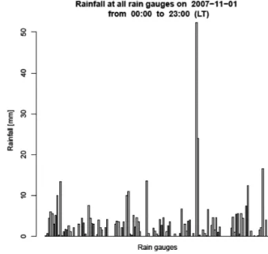
The UDFplot withinHours()(Appendix)uses UDF 1 and UDF 7(Appendix). By calling the UDFs: plot withinDays(), plot withinMon-ths(), and plot withinYears() it is possible to change the granularity of the diagram. The barplot in Figure 5 shows the rainfall regis-tered at each rain gauge in the Lazio region on 2007-11-01, from 00:00 to 23:00. The diagram is built by running the command:
SELECT barPlot withinHours(’2007-11-01’,
’00:00’, ’23:00’,
’barPlot withinHours.pdf’)
Each bar of the graph represents the precipita-tion accumulated in a rain gauge in the specified twenty-three hours.
To deepen the knowledge about the data behind the diagram of Figure 5, it would be sufficient to make recourse to the querying. Unfortunately, it is not reasonable to assume that nontechnical users have such a skill. But, we can help them by creating the viewrgwithinlaziothat hides in its “body” most details(namely, the need to look at three of the four database tables and join two of them, as well as the need to call the spa-tial operator ST Contains() and the function SUM).
Figure 5.Time series of the precipitation measured by the rain gauges within Lazio on the 1stof November
CREATE VIEW rgwithinlazio AS (
SELECT rg.id gauge ,rg.name, rg.location, SUM(accumulated) as accumulated
FROM precipitation AS p, rain gauge AS rg, region AS r
WHERE p.gauge=rg.id gauge AND
ST Contains(r.boundary, rg.location)=true AND
r.name=’LAZIO’ AND p.date=’2007-11-01’ AND
p.time > ’00:00’ AND p.time < ’23:00’
GROUP BY rg.id gauge, rg.name, rg.location );
After a short on-the-job training, nontechnical users, by calling such a database object, may become able to formulate non-trivial queries such as, for instance, to count the stations that have measured a rainfall above a given threshold
(e.g., 13 mm)on 2007-11-01:
SELECT count(id gauge)
FROM rgwithinlazio
WHERE accumulated > 13;
or display the identifier, name and geographic position of those stations:
SELECT id gauge name, location
FROM rgwithinlazio
WHERE accumulated > 13;
The output of this second query can be displayed in the usual tabular format(Figure 6)as well as a map(Figure 7).
Figure 6.The table collecting the identifier, name and geographic position of the rain gauges within Lazio that
measured, on the 1stof November 2007, a precipitation
volume above 13 mm.
Figure 7.The(QGIS)map about the rain gauges within Lazio that measured, on the 1stof November 2007, a
precipitation volume above 13 mm.
The UDFs rainfallPlot withinHours(), rainfallPlot withinDays(),rainfallPlot withinMonths(),rainfallPlot withinYears() build diagrams that bring the progressive sum of the precipitation recorded in the time interval specified, as well as that fallen every 15 min-utes.
6.5. Interpolation
In the reality, one always has to estimate the value of environmental variables from a limited set of measurements. For this reason many spa-tial interpolation methods have been developed. IDW and kriging are the best known methods
(Li and Heap, 2008). As pointed out by Bostan et al.(2012), spatial interpolation methods have been applied to precipitation measurements on daily, monthly and annual averages. TheIDW,
6.5.1. IDW
This method is based on the physical law that everything is related to everything else, but near things are more related than distant things. IDW is one of the simplest and most popular interpo-lation techniques(Li and Heap, 2008).
The IDW method is very effective when ap-plied to precipitation data, under the condition that the optimal exponent(p) is identified(Lu and Wong, 2008),(Li et al., 2011),(Keblouti et al., 2012),(Chen and Liu, 2012). It is possible to determine the optimal value ofpminimizing the Root Mean Squared Error(RMSE).
TheIDWpackage allows to interpolate the mea-sured data(and collected in the table precipi-tation), adopting the four levels of granularity mentioned in Section 4. For example, via the UDFidw whithinDays()(Appendix), it is pos-sible to apply the IDW method to the values of the precipitation accumulated in an arbitrary number of days. TheCrossValidationpackage supports the calculation of the RMSE through four routines referring to the four different tem-poral granularities supported by the packages of Table 3.
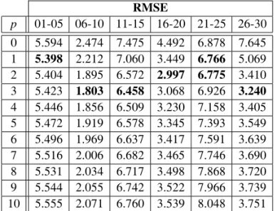
Through the UDFidw crossValidation with-inDays()(Appendix), we calculated the RMSE for values of p ranging between 0 and 10, for six distinct daily intervals: 01-05, 06-10, 11-15, 16-20, 21-25 and 26-30 of November 2007. The numerical results are collected in Table 5. It shows that values ofpbetween 1 and 3 return a very low error for each of the six time intervals
RMSE
p 01-05 06-10 11-15 16-20 21-25 26-30 0 5.594 2.474 7.475 4.492 6.878 7.645 1 5.398 2.212 7.060 3.449 6.766 5.069 2 5.404 1.895 6.572 2.997 6.775 3.410 3 5.423 1.803 6.458 3.068 6.926 3.240
4 5.446 1.856 6.509 3.230 7.158 3.405 5 5.472 1.919 6.578 3.345 7.393 3.549 6 5.496 1.969 6.637 3.417 7.591 3.639 7 5.516 2.006 6.682 3.465 7.746 3.690 8 5.531 2.034 6.717 3.498 7.868 3.720 9 5.544 2.055 6.742 3.522 7.966 3.739 10 5.555 2.071 6.760 3.539 8.048 3.751
Table 5.The RMSE values for differentpvalues.
considered. This result is in line with the find-ings of studies already conducted. For instance, Chen and Liu(2012)found that the optimal ex-ponent value varies between 0 and 5; Ahani et al. (2012) report a case study on precipitation in Iran for a period of 33 years for which they found that the optimum value ofpis 2.
Set p = 2, nx = ny = 300 (to know about
nx and ny please refer to the Appendix), we got(by usingidw whithinDays())the maps of the rainfall over Lazio, for the entire month of November 2007(Figure 8).
Figure 8.The raster map of the total precipitation volume over Lazio, in November 2007.
Before closing the section, we propose a com-parison between the raster map in Figure 8, with that obtained by using QGIS(Figure 9). As can be seen, the two maps are almost identical.
7. Conclusions
The adopted solution setting aims at encour-aging nontechnical users, after a short on-the-job training, to manipulate by themselves the measurements coming from rain gauges located over a geographical area. The involved stake-holders are only required to familiarize with the objects that the SDB exposes and invoke their execution.
Our vision for the near future hopes that na-tional agencies with the responsibility of land government(in the case of Italy the Department of Civil Protection)will make available period-ically (e.g. on an annual basis)an SDB about the historical rainfall data, enhanced with a wide repertoire of objects(viewsand UDFs)oriented to analyse those data. In addition to the SDB, it will be sufficient to provide a user’s guide so that anyone who has the desire or the need can take advantage of this service to perform stud-ies focused on the portions of the territory of his interest.
Last but not least, it is worthwhile to point out that the solution framework we have imple-mented to carry out the experience reported in the paper can be replicated in other areas of high social impact that involve large spatio-temporal data, keeping the operational effectiveness un-altered.
References
[1] H. AHANI ET AL., An investigation of trends in precipitation volume for the last three decades in different regions of Fars province, Iran.Theoretical and Applied Climatology,109(2012), 361–382.
[2] P. A. BOSTAN, G. B. M. HEUVELINK, S. Z. AKYUREK, Comparison of regression and kriging techniques for mapping the average annual precip-itation in Turkey.International Journal of Applied Earth Observation and Geoinformation,19(2012), 115–126.
[3] D. J. BURNETTE, D. W. STAHLE, Computer assisted screening, correction, and analysis of historical weather measurements.Computers & Geosciences,
54(2013), 309–317.
[4] A. J. CANNON, Quantile regression neural networks: Implementation in R and application to precipita-tion downscaling, Computers & Geosciences, 37
(2011), 1277–1284.
[5] C. J. CARLETON, R. A. DAHLGREN, K. W. TATE, A relational database for the monitoring and analy-sis of watershed hydrologic functions: I. Database design and pertinent queries. Computers & Geo-sciences,31(2005), 393–402.
[6] F. W. CHEN, C.-W. LIU, Estimation of the spatial rainfall distribution using inverse distance weight-ing (IDW) in the middle of Taiwan. Paddy and Water Environment,10(2012), 209–222.
[7] U. HABERLANDT, Geostatistical interpolation of hourly precipitation from rain gauges and radar for a large-scale extreme rainfall event.Journal of Hydrology,332(2007), 144–157.
[8] T. HENGL, A Practical Guide to Geostatistical Mapping. Office for Official Publications of the European Communities, Luxembourg, 2009.
[9] M. KEBLOUTI, L. OUERDACHI, H. BOUTAGHANE, Spatial Interpolation of Annual Precipitation in Annaba-Algeria – Comparison and Evaluation of Methods.Energy Procedia,18(2012), 468–475.
[10] J. LI, A. D. HEAP, A Review of Spatial Interpolation Methods for Environmental Scientists.Geo-science Australia Record,23(2008), 137.
[11] Q. LI, Y. CHEN, Y. SHEN, X. LI, J. XU, Spatial and temporal trends of climate change in Xinjiang, China. Journal of Geographical Science, 21(6) (2011), 1007–1018.
[12] G. Y. LU, D. W. WONG, An adaptive inverse-distance weighting spatial interpolation technique. Comput-ers & Geosciences,34(2008), 1044–1055.
[13] E. J. PEBESMA, Multivariable geostatistics in S: the gstat package. Computers & Geosciences, 30
(2004), 683–691.
[14] J. POKORNY, Database architectures: Current trends and their relationships to environmental data man-agement.Environmental Modelling & Software,21
(2006), 1579–1586.
[15] P. ROWHANIA, D. B. LOBELL, M. LINDERMANC, N. RAMANKUTTYA, Climate variability and crop pro-duction in Tanzania.Agricultural and Forest Mete-orology,151(2011), 449–460.
[16] J. SHEN, A. PARKER, J. RIVERSON, A new approach for a Windows-based watershed modeling system based on a database-supporting architecture. En-vironmental Modelling & Software, 20 (2005), 1127–1138.
[17] S. STEINIGER, E. BOCHER, An Overview on Current Free and 61 Open Source Desktop GIS Devel-opments. International Journal of Geographical Information Science,23(2009), 1345–1370.
[18] H. TABARI, P. H. TALAEE, Temporal variability of precipitation over Iran: 1966–2005. Journal of Hydrology,396(2011), 313–320.
Received:January, 2014
Revised:May, 2014
Accepted:June, 2014
Contact addresses:
Paolino Di Felice Department of Ingegneria Industriale e dell’Informazione ed Economia University of L’Aquila Italy e-mail:[email protected]
Luca Finocchio Daniele Leombruni Vittoriano Muttillo Master students in Engineering Informatics University of L’Aquila Italy
PAOLINODIFELICEis a professor of computer science at the Department of Industrial and Information Engineering & Economics of the Univer-sity of L’Aquila, since 1999. He has authored or co-authored about 100 articles in international journals, books, and conference proceed-ings in the areas of programming methodologies, relational and spatial databases. He has also carried out a consistent activity of technolog-ical transfer in collaboration with several IT firms. His research has been funded by national and international institutions and carried out in collaboration with researchers from several countries(Italy, Holland, Germany, and the USA). He has served within national and interna-tional committees. For the last few years, he has been a regular member of the program committee of the International Conference on Integrated Information(IC-ININFO).
LUCAFINOCCHIO, DANIELELEOMBRUNI ANDVITTORIANOMUTTILLO
Appendix
The SQL/DDL statements to create the four tables of the SDB (Section 3).
CREATE TABLE rain gauge (
id gauge integer PRIMARY KEY,
name character varying(50),
num station integer,
location geometry);
CREATE TABLE precipitation (
gauge integer,
date date,
time time,
accumulated double precision, PRIMARY KEY (gauge, date, time),
FOREIGN KEY (gauge) REFERENCES Rain gauge(id gauge) ON DELETE NO ACTION ON UPDATE CASCADE );
CREATE TABLE region (
id region integer PRIMARY KEY,
name character varying(50),
boundary geometry );
CREATE TABLE district (
id district integer PRIMARY KEY,
region integer,
name character varying(50),
boundary geometry,
FOREIGN KEY (region) REFERENCES Region(id region) ON DELETE RESTRICT ON UPDATE CASCADE );
The remainder of this appendix collects the code of some of the UDFs mentioned in Section 5.
The UDFimport precipitation().
It migrates the data about the rain measurements into tableprecipitation.
Inputs:
• path(text): path to reach the file of the measurements data
• date(text): month to which the measurements refer(date format: yyyy-mm). CREATE OR REPLACE FUNCTION import precipitation(path text, date text) RETURNS void AS
$BODY$
INSERT INTO precipitation (gauge, date, time, accumulated)
SELECT gauge, date, time, accumulated
FROM UDF 0(path, date)
t(gauge integer, time time, station text, accumulated double precision, date date) $BODY$
LANGUAGE SQL
UDF 1
It calculates the sums of the progressive accumulated rain every 15 minutes in a given rain gauge in a predetermined interval of hours of a specific day.
Inputs:
• gauge name(text): name of the rain gauge
• day(text): the day of interest
• from h(text): the initial hour
• to h(text): the final hour
Output:
A set of tuples of typerainfall.
rainfall is a user data type defined as follows: CREATE TYPE rainfall AS (
date date,
time time without time zone,
sum double precision )
The PL/pgSQL code:
CREATE OR REPLACE FUNCTION UDF 1(gauge name text, day text, from h text, to h text) RETURNS SETOF rainfall AS
$BODY$ DECLARE
row precipitation%rowtype;
result rainfall;
BEGIN
result.sum=0; FOR row IN
SELECT *
FROM precipitation AS d, rain gauge AS r
WHERE r.id gauge=d.gauge AND r.name=gauge name AND d.date=CAST(day as date) AND
d.time BETWEEN CAST(from h as time) AND CAST(to h as time) ORDER BY d.time
LOOP
result.date=row.date; result.time=row.time; IF row.accumulated IS NOT NULL THEN
result.sum=result.sum+row.accumulated; ELSE
result.sum=result.sum; END IF;
RETURN NEXT result; END LOOP;
RETURN; END
$BODY$
UDF 7
It returns a .pdf file containing the chart with the hours on the x-axis and the amount of rainfall measured(mm)on they-axis.
Inputs:
• path (text): path of the(.pdf)file to be created
• gauge name (text): name of the pluviometer of interest
• x1 (time[]): array about the time of sampling
• y (double precision[]): array of the measurements
Output:
A boolean value: trueif the pdf file has been created,falseotherwise
The PL/R code:
CREATE OR REPLACE FUNCTION UDF 7(path text, gauge name text, date text, x1 time without time zone[], y double precision[]) RETURNS boolean AS
$BODY$
x2 <- strptime(x1, format=’%H:%M’); x <- as.double(x2);
l <- length(x); pdf(path);
plot(x, y, xlab=’Time (LT) [hh-mm-ss]’, ylab=’Rainfall [mm]’,
main=paste(’Rainfall at’, gauge name, ’ rain gauge on ’, date), xaxt=’n’); axis(1, at=c(x[1], x[l/2],x[l]), labels=c(x1[1], x1[l/2], x1[l]));
lines(x, y, col=’blue’, lwd=2);
legend(x[1], max(y), c(’Rainfall Value’,’ Zigzag Curve’), lty=c(-1,1), pch=c(1,-1), col=c(’black’, ’blue’), lwd=c(-1,2), merge=TRUE);
dev.off(); return (TRUE); $BODY$
LANGUAGE ’plr’;
The UDFplot withinHours()
It plots the sum of the rainfall accumulated every 15 minutes in a rain gauge in a range of hours of a given day. The drawing is returned as a .pdf file.
Inputs:
• path (text): path of the(.pdf)file to be created
• gauge name (text): name of the rain gauge
• from h(text): the initial hour
• to h(text): the final hour
Output:
The PL/pgSQL code:
CREATE OR REPLACE FUNCTION plot withinHours(path text, gauge name text, day text, from h text, to h text)
RETURNS boolean AS $BODY$
DECLARE
r rainfall; x time[];
y double precision[]; i integer=1;
BEGIN
FOR r IN SELECT *
FROM UDF 1(gauge name, day, from h, to h) LOOP
x[i]=r.time; y[i]=r.sum; i=i+1; END LOOP;
RETURN UDF 7(path, gauge name, x, y); END
$BODY$
LANGUAGE ‘plpgsql’;
The UDFidw withinDays()
It interpolates, by means of the IDW technique, the rain accumulated in all the rain gauges in a given interval of days within a given region (in our case, eitherLazio or Umbria). A geocoded
(.asc)raster file is returned. This function calls four(Auxiliary)UDFs. The(PLpgSQL)UDF 4 computes the sum of the precipitation accumulated by all the rain gauges in the given interval of days within the given region. The (PL/R) UDF 14 computes the interpolation grid, given the dimensions and the coordinatesxandyof a square. The(PLpgSQL)UDF 15 filters the points of the grid returned by UDF 14 within the given region. The(PL/R)UDF 16 interpolates, by calling the functionidwof the librarygstat, the data received as inputs and returns a geocoded(.asc)raster file built by linking the functionrasterof the libraryraster.
Inputs:
• region name (text): name of the region of interest(either Lazio or Umbria)
• from d (text): the initial day
• to d (text): the final day
• path (text): path of the(.pdf)file to be created
• power (double precision): value of the exponent of the IDW method
• nx (int): number of points of the grid along thex-axis
• ny (int): number of points of the grid along they-axis
Output:
The PL/pgSQL code:
CREATE OR REPLACE FUNCTION idw whithinDays(region name text, from d text, to d text, path text, power double precision, nx integer, ny integer) RETURNS integer AS
$BODY$ DECLARE
id gau integer[];
gauge na character varying(50)[]; acc double precision[];
row record;
x double precision[]; y double precision[]; i integer;
row1 record;
xg double precision[]; yg double precision[]; ig integer;
row2 record;
xgf double precision[]; ygf double precision[]; igf integer;
BEGIN i=0; FOR row IN
SELECT id gauge AS id, gauge name AS name, sum AS a,
ST X(location) AS xx, ST Y(location) AS yy
FROM UDF 4(from d, to d)
LOOP
id gau[i]=row.id; gauge na[i]=row.name; x[i]=row.xx;
y[i]=row.yy; acc[i]=row.a; i=i+1; END LOOP;
ig=0; FOR row1 IN
SELECT *
FROM UDF 14(11, 14.5, 40.5, 44, nx, ny)
t(xgrid double precision, ygrid double precision) LOOP
xg[ig]=row1.xgrid; yg[ig]=row1.ygrid; ig=ig+1;
END LOOP;
igf=0; FOR row2 IN
SELECT *
FROM UDF 15(region name, xg, yg)
LOOP
xgf[igf]=row2.xgridfilter; ygf[igf]=row2.ygridfilter; igf=igf+1;
END LOOP;
RETURN UDF 16(id gau, gauge na, x, y, xgf, ygf, acc, power, path); END;
$BODY$
LANGUAGE plpgsql;
The UDFidw crossValidation withinDays()
It performs the cross validation of the IDW method, run by changing the value of the exponent. All the interpolations refer to the same interval of days given as input. The cross validation is coded inside the (PL/R) UDF 17, which calls specific gstat functions that carry out the actual computations.
Inputs:
• from d (text): initial day
• to d (text): final day
• from p (double precision): lower bound of the exponent
• to p (double precision): upper bound of the exponent
• by p (double precision): step of increment of the exponent
Output:
A set of records about the RMSE for each exponent value.
The PL/pgSQL code:
CREATE OR REPLACE FUNCTION idw crossValidation withinDays(from d text, to d text, from p double precision, to p double precision, by p double precision) RETURNS SETOF record AS
$BODY$ DECLARE
id gau integer[];
gauge na character varying(50)[]; acc double precision[];
row record;
x double precision[]; y double precision[]; i integer;
row1 record; ret power RMSE; BEGIN
i=0; FOR row IN
SELECT id gauge AS id, gauge name AS name, sum AS a,
ST X(location) AS xx, ST Y(location) AS yy
LOOP
id gau[i]=row.id; gauge na[i]=row.name; x[i]=row.xx;
y[i]=row.yy; acc[i]=row.a; i=i+1;
END LOOP; FOR row1 IN
SELECT *
FROM UDF 17(id gau, gauge na, x, y, acc, from p, to p, by p)
t(idp double precision, val double precision) LOOP
ret.power =row1.idp;
ret.RMSE =row1.val;
RETURN next ret; END LOOP;
END; $BODY$