*Correspondence to Author:
Guozhu Chen
College of Hydraulic & Environmen- tal Engineering, China Three Gorg-es University, Yichang, 443002, C-hina.
How to cite this article:
Xiaoxi Men, Guozhu Chen, Xiaoxiong Zuo, Haijun Guo. A mathematical
model for grading clouds to study solar flares based on fuzzy c-means algorithm. American Journal of Basic and Applied Sciences, 2019, 2:10
eSciPub LLC, Houston, TX USA. Website: http://escipub.com/
Xiaoxi Men et al., AJBAS, 2019 2:10
American Journal of Basic and Applied Sciences
(ISSN:2637-6857)
Research Article AJBAS (2019) 2:10
A mathematical model for grading clouds to study solar flares
based on fuzzy c-means algorithm
In this paper, a cloud-level grading comprehensive evaluation
model based on fuzzy c-means algorithm is established. The image is binarized by the maximum inter-class variance method to obtain the dim curve. According to the dim curve of the four quadrants, the distribution and thickness of the cloud layer are discriminated. Three attributes of the effective area of the cloud layer, the total amount of clouds, and the thickness of
the cloud amount are selected as the characteristic data of the comprehensive evaluation model.
Keywords: Dim curve; Fuzzy c-means algorithm; Cloud grading.
Xiaoxi Men1, Guozhu Chen2*, Xiaoxiong Zuo3, Haijun Guo2
1.College of Electrical Engineering & New Energy, China Three Gorges University, Yichang,
443002, China. 2.College of Hydraulic & Environmental Engineering, China Three Gorges University, Yichang, 443002, China. 3.College of Science, China Three Gorges University, Yichang, 443002, China.
1. Introduction
The solar flare is a violent explosion that occurs inside the solar atmosphere. It releases a large amount of energy quickly in a short period of time, causing local areas to be instantly heated, emitting various electromagnetic radiation out-wards, and the surrounding particles are en-hanced. It is generally believed that the flare is produced by the rapid release of the magnetic field energy of the active area near the sunspot. Flare occurs when the magnetic field of the sun-spot produces a magnetic field of another small-scale special structure.
Long-term observations indicate that most of the flare phenomenon occurs between the low corona zone above the sunspot group and the top atmosphere of the sun chromosphere. And the more complex the sunspot group structure, the higher the probability of occurrence of large flares. A normally developing sunspot will pro-duce a flare on average for a few hours.
In recent years, most researchers have favored the study of flare phenomena. But the photo-graphs of the flares obtained must be processed before they can be used for research because the observations are often occluded by clouds. According to above, a mathematical model is established to classify the amount of clouds to study solar flares.
2. Model Preparation
2.1 Extraction of Data Features
After analyzing the data characteristics of the solar flare, three attribute characteristics of the cloud amount are obtained, which are the effec-tive area of the cloud layer, the total amount of the cloud, and the difference in the thickness distribution of the cloud amount. And they are defined as follows.
Effective area of the cloud: We select the cloud amount of the baseline as a reference. The cloud amount is the difference between the amount of cloud before the filtering and the amount of cloud after the guided filtering. We compare the cloud amount of each pixel of the sample to be tested with the reference cloud of the corresponding pixel, and the area of the pixel above the reference cloud is considered valid.
Total amount of clouds: The sum of the clouds at each pixel of the sun's full-day map.
amount: Since the cloud amount of each pixel on the full-day map is regionally distributed, in order to show the difference of regional distribu-tion, the variance of each region is selected to show the difference of cloud amount.
2.2 Data Standardization
Since the dimensions of these three attributes are different, the data needs to be normalized first. Standardization refers to removing the unit limit of the data and converting it into a dimen-sionless, pure value so that indicators of differ-ent units or magnitudes can be compared and weighted. The basic idea of using standardized processing is to standardize data based on the quotient division of the maximum and minimum values of the original data. The expression is as follows.
min max min
x x
x
x x
− =
−
In the above formula, a represents sample data before unnormalized processing, and b is data after normalization processing.
2.3 Solving the Dim Curve of the Edge
Dimness on the edge means that the brightness of the sun's round surface gradually darkens from the center of the sun to the edge of the sun. We can observe the solar surface cloud distri-bution and the general situation or specific loca-tion of the flare distribuloca-tion by observing the dark curve of the edge, thus facilitating the sub-sequent cloud processing.
1)Binary Image
AJBAS: https://escipub.com/american-journal-of-basic-and-applied-sciences/ 3
The gray value of the full-day sun image is be-tween 0 and 255, which we normalize to 0 to 1. Using MATLAB software, the maximum
inter-class variance method is used to automatically calculate the threshold value is approximately
equal to 0.3608, so the gray value of the full-day solar image is binarized. When the gray value is greater than 0.3608, it is taken as 1, and when the gray value is less than 0.3608, it is taken as 0. We take a flare image and after the above processing, the image is got (Fig. 1).
Fig. 1: The image after binarization
As can be seen from Fig. 1, the periphery of the sun is black, the sun is white, that is, the sur-rounding gray value is zero, and the sun gray value is one.
2)Edge Extraction
The edge extraction of binary images does not require complex operators. Here we use the so-bel operator to convolve with the binary image, and the result is the edge of the image, which is shown in Fig. 2.
Fig. 2: Edge Extraction Diagram 3)Fitting the Image Contour to Find the Center and Radius
After obtaining the coordinates of each point on the edge of the image, in order to obtain the center and radius, a circle fitting is required. The basic idea is the least squares method.
The analytical equation of the circle is expressed as follows.
2 2 2
(x−xc) +(y−yc) =R
According to the idea of the least square’s method, the following definitions are made.
2 2 2 2
(( c) ( c) )
f =
x−x + y−y −Rof f be zero, the variance is maximized, and the expression is expressed as follows. 0 0 0 c c f x f y f R = = =
Solve the above formula, the result is as follows.
2 2 2
(( ) ( ) )
c c c c
i c i c
x u x
y v y
R x x y y
= + = + = − + −
In the above formula, ( ,x yc c)is the center of the circle and Ris the radius.
2
2
2( )
2( )
uuv uv uuu vv uvv vv uv vvv c
uv uu vv
uu uuv uuu uv uv uvv uu vvv c
uv uu vv
S S S S S S S S
u
S S S
S S S S S S S S
v
S S S
− − + = − − + + − = − − 3 3 2 2 2 2 uuu i vvv i uu i vv i uv i i uuv i i uvv i i
S u
S v
S u
S v
S u v
S u v
S u v
= = = = = = =
i i c c i i c cu x x
u x x
v y y
v y y
= − = − = − = −
4)Panning the Center of the Circle to the Center of the Image
In order to facilitate the subsequent operation, after acquiring the center of the circle and the radius, we remove the information outside the circle firstly, and then shift the center of the circle to the center of the image. The solar flare pattern at this time is symmetrical along the central axis, and the effect diagram is shown in Fig. 3.
AJBAS: https://escipub.com/american-journal-of-basic-and-applied-sciences/ 5
5)Polar Coordinate Transformation
In order to obtain the dim curve of the image, it is necessary to first convert the image from a Car-tesian coordinate system to a polar coordinate system. Direct conversion is not convenient, so we use the rotation sampling method to convert. First, select the gray value in one direction of the original image as the first column of the polar coordinate image, then rotate the whole image around the center by a small angle, and extract again in the same direction, and repeat this step several times. Until the entire image is turned over one week, the resulting data is a matrix and is the image in polar coordinates.
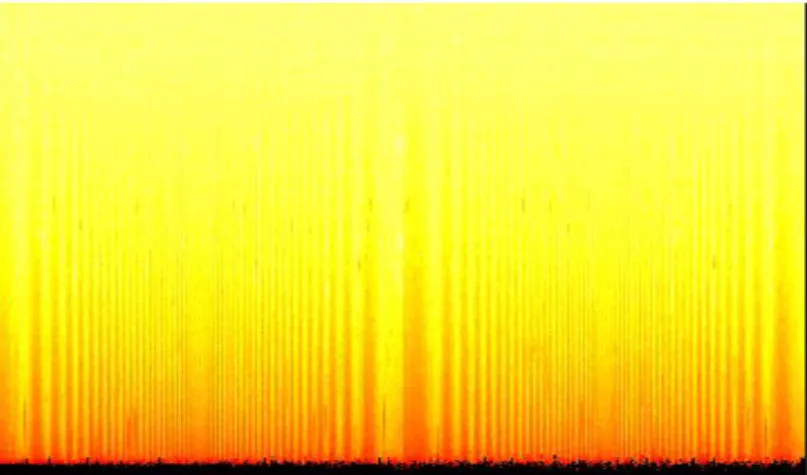
Fig. 4: Full sun image of the sun in polar coordinates 6)Getting the Dim Curve
The image in polar coordinates is divided into four quadrants, and they are averaged to obtain the average edge dim curves of the four quad-rants.
The vertical coordinate pixel value of the dim curve of the edge reflects the brightness of each point different from the distance from the center of the circle. Therefore, the position of the steep drop indicates the edge of the sun, and the brightness drops sharply. The concave portion of the curve indicates a decrease in brightness, indicating that there is a cloud here. The convex portion of the curve indicates a sharp increase in brightness, indicating that there is a flare here. 3. Model Establishment
The basis of the C-means algorithm is the mini-mum error squared criterion. If Ni is the
num-ber of samples in the cluster iand mi is the
mean of these samples, and the expression is as follows.
1
i
i y
m y
N
=
The sum of squared errors between each sam-ple y in i and the mean mi is added as
fol-lows.
2 1
( )
i
C
e i
i y
J y m
=
=
−e
J is the squared error sum clustering criterion,
which is a function of the sample set Yand the
category set . For different clusters, the error square Je is also different, and the smallest
er-ror square Je is the optimal result. The
imple-mentation of Je minimization uses iterative
methods to continually adjust the categories of samples. After this adjustment, the mean values of the two types are expressed as follows.
1
1
k k j
k j j j
j
m y
m m
N
y m
m m
N
−
= +
− −
= +
+
Correspondingly, the sum of the squared errors of the two types is also expressed as follows.
2
2
( )
1
( )
1
k k k k
k j j j j
j
N y m
J J
N
N y m
J J
N
−
= −
− −
= +
+
2 2
( ) ( )
1 1
j j k k
j k
N y m N y m
N N
− −
4. Cloud Grading
Based on the above model, we divide the cloud amount into five levels, and the names and characteristics are as follows.
Non-uniform cloud: Clouds are unevenly distrib-uted and have very little cloud.
Non-uniform and thin cloud: Clouds are less un-evenly distributed and have less cloud distribu-tion.
Thin cloud in the central area: A small amount of clouds are mainly distributed in the central area.
Thick clouds in small area: Small areas have thick clouds.
Thick clouds in large area: Large areas have thick clouds.
5. Conclusion and Outlook
In this paper, the classification of the model is considered comprehensive, including not only the thickness information of the cloud layer, but also the position information and the change of
the thickness of the cloud layer with the position. At the same time, we can use the dim curve to identify whether there is a cloud. For the c-means dynamic clustering algorithm adopted, it has strong universality and is involved in the fields of classification and pattern recognition. And we use the three-dimensional c-means clustering algorithm, which can be extended to high-dimensional space to solve more complex problems, and also has higher precision.
References
1. G. Petschnigg, M. Agrawala, H. Hoppe, R.
Szeliski, M. Cohen, andK. Toyama, “Digital Photography with Flash and No-Flash Image-Pairs,” Proc. ACM Siggraph, 2004.
2. C. Tomasi and R. Manduchi, “Bilateral Filtering
for Gray and Color Images,” Proc. IEEE Int’l Computer Vision Conf., 1998.
3. Kaiming He, Jian Sun, Xiaoou Tang, Guided