Vol. 10, No. 5, 2017, 1092-1098 ISSN 1307-5543 – www.ejpam.com Published by New York Business Global
On the Error Analysis of a Continuous Implicit Hybrid
One Step Method
T. A. Anake1,∗, S. O. Edeki1
1 Department of Mathematics, Covenant University, Canaanland, Ota, Nigeria
Abstract. It is a known fact that in the application of a continuous linear multistep method, the global error at a particular point is influenced by the accumulation of local truncation errors at each step from the initial point and thereby reduces the accuracy of the approximated result. Hence, by controlling the growth of local errors it is expected that the accuracy of the approximations should improve. In this paper therefore, a method is derived for the bound on the local truncation error of continuous implicit hybrid one step method for the solution of initial value problems of second order ordinary differential equations by means of the generalized Lagrange form of the Taylor’s remainder and the mean value theorem.
2010 Mathematics Subject Classifications: 34K34, 65L70, 34A45
Key Words and Phrases: truncation error, global error, mean value theorem, remainder theo-rem, one step method, hybrid multistep method
1. Introduction
An important property associated with the numerical solutions of the initial value problems of ordinary differential equations (ODEs), is the global error of computation. The size of this error on the interval of interest makes the effort put into developing the numerical method worthwhile or futile. If the global error is small, the numerical solution is considered to be accurate, and other properties of the solution become less important.
The requirement of a small global error will guarantee that the dynamics of the ap-proximate solution is similar to that of the exact solution and facilitate step size control using the global error estimate, (Orel,2010).
The relationship between the local and the global errors and possible ways of control-ling the global error directly has attracted a lot of interest. A number of researchers have studied this situation for different numerical methods; for instance, Highhman(1993), Dor-mundet al.(1994), Calvoet al.(1996) and Stuart(1997) all studied the connection between local truncation error and global error for Runge-Kutta methods while Lambert(1979),
∗
Corresponding author.
Email addresses: [email protected](T. A. Anake),[email protected](S. O. Edeki)
Onumayiet al.(1999) as well as Kulikov and Shindin(2004) were concerned with estimates of these errors for multistep methods.
It is a well known that in the application of a linear multistep method at any given point, sayxi, the global error would usually be an accumulation of the local errors
com-mitted at each step from the initial point up to the reference point. This is usually a function of the problem to be solved, the numerical method adopted and step size se-lected, (Orel,2010). However, while it may be possible to control the local errors and step size during the implementation of the linear multistep method, it may not be possible to do the same for the global error directly.
The aim of this paper is to derive a method for a bound on the local truncation error, at each step of application, of a continuous implicit hybrid one step method(CIHOSM) as a means of managing the magnitude of the global error of computation. The result presented in this paper, extends an earlier result by Lambert(1979) for special second order initial value problems to the general case.
The paper is organized as follows: in Section 2 the CIHOSM is introduced. The main result is presented in Section 3. The error bound method derived in Section 3 is applied on the CIHOSM proposed in Anake and Adoghe(2013) for the solution of a simple electric circuit problem using different step sizes in Section 4. Finally in section 5, conclusions are presented.
2. The Continuous Implicit Hybrid One Step method
Consider the general form of the continuous implicit hybrid one step method proposed by Anake and Adoghe(2013):
y(x) = X
j0=r−1,r
ανj0(t)yn+νj0 +h
2
1 X
j=0
βj(t)fn+j + r
X
j0=1
βνj0(t)fn+νj0
, (1)
where αν0
j βν
0
j and βj are continuous in t ∈; yn+j is the numerical approximation of the
exact solution at the grid point xn+j, and fn+j = f(xn+j, yn+j, yn0+j). The subscript,
νj0 ∈(0,1), ∀j0 is a rational number representing thej0th off-grid point.
We note that by using off-grid points, the method mimics a continuous implicit mul-tistep method and solves directly ordinary differential equations of the form:
y00=f(x, y, y0)
y(a) =η0, y0(a) =η1
(2)
wherex∈[a, b], a, b∈and f is continuously differentiable with respect to its arguments. Ordinary differential equations such as (2) are important in many application areas (see, Chapra and Canale(2010), Anake(2011)).
Definition 1 ([Anake,2011, p.61] Local Truncation Error). The local truncation error at xn+k of the numerical method (2) is defined to be the operator L[y(xn);h] given by:
L[y(xn);h] = k
X
j=0
αjy(xn+jh)−h2βjy00(xn+jh)
(3)
when y(xn) is the theoretical solution of the initial value problem (2)at xn.
In what follows, we shall assume that in the application of the method (1) to yield
yn+k, no previous truncation errors have been made. Furthermore, we shall assume the
theoretical solutiony(x) possessesp+2 continuous derivatives, so that the local truncation error has the value;
L[y(xn);h] =Cp+2hp+2yp+2(xn) +O(hp+3) (4)
wherepandCp+2 are taken to be the order and error constant of method (1) respectively.
Theorem 1 ([Huang,2001, p.2] Generalized Mean Value Theorem). If ϕ is continuous and ϑ is integrable on an interval containing a and x, and ϑ does not change sign in the interval [a, x], then there exists a point ζ between aand x such that
Z x
a
ϕ(t)ϑ(t)dt=ϕ(ζ)
Z x
a
ϑ(t)dt. (5)
We note that the asymptotic method (4) can only predict the behaviour of the error in the limit ash→0. Furthermore, our knowledge of the orderpand error constant Cp+2 of
the method is not sufficient to deduce a bound for the magnitude of the local truncation error when h is fixed, since the magnitude of the termO(hp+3) is unknown.
3. Main Result
We present the main result as a proposition as follows.
Proposition 1. Given the operator L, of order p and error constant Cp+2, for h fixed, the local truncation error takes the form:
L[y(xn);h] =Cp+2hp+2yp+2(xn+ξh), 0< ξ < k (6)
and
|L[y(xn);h]| ≤hp+2QY (7)
where
Q=|Cp+2|=
1
p!
Z k
0
G(t)dt
(8a)
and
Y = max
x∈[a,b]|y
Proof. Define the generalized form of the Lagrange remainder Rp+1 afterp+ 2 terms
in a Taylor expansion of a sufficiently differentiable function G(x) about x=aas;
Rp+1=
1 (p+ 1)!
Z h
0
(h−z)p+1G(p+2)(a+z)dz. (9)
Then we can now write the Taylor expansions of y(xn+jh) about xn truncated after
p+ 2 terms as
y(xn+jh) =y(xn) +jhy(1)+
(jh)2 2! y
(2)(x
n) +· · ·+
(jh)p+1 (p+ 1)!y
(p+1)
+ 1
(p+ 1)!
Z jh
0
(jh−z)p+1y(p+2)(xn+z)dz
(10)
and in the same manner, the Taylor expansion ofy00(xn+jh) aboutxntruncated after p
terms may now be written as
y(2)(xn+jh) =y(2)(xn) +jhy(3)+
(jh)2 2! y
(4)(x
n) +· · ·+
(jh)p−1 (p−1)!y
(p+1)
+ 1
(p−1)!
Z jh
0
(jh−z)p−1y(p+2)(xn+z)dz.
(11)
Makingz=th, (10) and (11) respectively become
y(xn+jh) =y(xn) +jhy(1)+
(jh)2
2! y
(2)(x
n) +· · ·+
(jh)p+1
(p+ 1)!y
(p+1)
+ h
p+1
(p+ 1)!
Z j
0
(j−t)p+1y(p+2)(xn+th)dt
(12)
and
y(2)(xn+jh) =y(2)(xn) +jhy(3)+
(jh)2 2! y
(4)(x
n) +· · ·+
(jh)p−1 (p−1)!y
(p+1)
+ h
p−1
(p−1)!
Z j
0
(j−t)p−1y(p+2)(xn+th)dt.
(13)
Then, using (12) and (13) in (3) yields after a little algebraic computation
L[y(xn);h] =
hp+2 p!
Z k
0
k
X
j=0
(p+ 1)−1αj(j−t)+p+1−pβj(j−t)p
−1 +
y(p+2)(xn+th)dt (14)
where
s+= (
s, ifs≥0,
Suppose the method is consistent, that is p≥1, also define the function F(t):
F(t) =
k
X
j=0
(p+ 1)−1αj(j−t)+p+1−pβj(j−t)p+−1
(16)
such that F(t) is a polynomial in each partition of the interval [0, k] and independent of the theoretical solutiony(x). Then, (14) can be written in terms of F(t) as follows:
L[y(xn);h] =
hp+2 p!
Z k
0
F(t)y(p+2)(xn+th)dt. (17)
Furthermore, assume thatF(t) does not change sign in the interval [0, k], then by Theorem 3.2, (17) becomes
L[y(xn);h] =hp+2
1
p!
Z k
0
F(t)dt
y(p+2)(xn+ξh), 0< ξ < k. (18)
Assume y(x) = xp+2, such that all derivatives of xp+2 of order greater than p+ 2 vanish identically. Then, by (18) and the expansion of the operator Lwe have;
Cp+2 =
1
p!
Z k
0
F(t)dt. (19)
Thus, (19) becomes
L[y(xn);h] =hp+2Cp+2y(p+2)(xn+ξh), 0< ξ < k (20)
which is the desired form. Hence,
|L[y(xn);h]|=|hp+2Cp+2y(p+2)(xn+ξh)| ≤ |hp+2||Cp+2| max
x∈[a,b]
|y(p+2)(x)|
∴ |L[y(xn);h]| ≤hp+2QY. (21)
4. Application of the Bound
Suppose the continuous implicit hybrid one step method proposed in Anake and Adoghe (2013), by evaluating (1) at the point xn+1, given as follows:
yn+1= 2yn+4 5
−yn+3 5+
h2
6000
h
18fn+1+ 209fn+4
5 + 4fn+ 3
5 + 14fn+ 2 5
−6fn+1 5 +fn
i , (22)
is implemented for the solution of the initial value problem:
Lq00+Rq0+ 1
Cq=E(t), q(0) = 0, q 0
with exact solution:
q(t) = 3 4−
3 4e
−10t(cos 10t+ sin 10t),
whereL= 1, C= 0.005, E(t) = 150 andR= 20. According to Anake and Adoghe(2013), application of the convergent method, of order p = 6, at the first grid point xn+1 yields
the local error constantCp+2 =−23625000000221 .
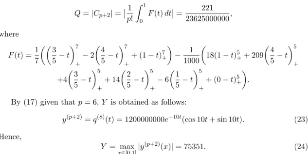
To apply (21), we will need to find Q, Y and choose a suitable step size. Thus, we checked that (19) is satisfied and the result of our computation agrees with the error constant reported by Anake and Adoghe (2013) as follows:
Q=|Cp+2|=
1
p!
Z 1 0
F(t)dt=
221 23625000000,
where
F(t) = 1 7
3 5 −t
7
+
−2
4 5 −t
7
+
+ (1−t)7+
− 1
1000
18(1−t)5++ 209
4 5−t
5
+
+4
3 5 −t
5
+
+ 14
2 5 −t
5
+
−6
1 5−t
5
+
+ (0−t)5+
.
By (17) given that p= 6,Y is obtained as follows:
y(p+2)=q(8)(t) = 1200000000e−10t(cos 10t+ sin 10t). (23)
Hence,
Y = max
x∈[0,1]|y
(p+2)(x)|= 75351. (24)
The bound on the application of the method (22) at the point xn+1 obtained for
different values of the step size h is shown in the table below:
Table 1: Different values ofhand the corresponding bound
h hp+2QY
0.003125 6.4108×10⁻²⁴ 0.01 7.0487×10⁻²⁰ 0.03 4.6247×10⁻¹⁶ 0.05 2.7534×10⁻¹⁴ 0.10 7.0487×10⁻¹²
5. Conclusion
that the magnitude of the bound computed reduces ash→0. This indicates that the size of the global error reduces with decrease in the step size and consequently, the accuracy of the approximation theoretically improves.
Acknowledgements
The authors are sincerely grateful to Covenant University for financial support and provision of good working environment. The referees’ helpful comments are highly appre-ciated.
References
[1] Anake, T.A.,Continuous Implicit Hybrid One Step Methods for the Solutions of Ini-tial Value Problems of General Second Order Ordinary DifferenIni-tial Equations, Ph.D Thesis, Covenant University, Canaanland, Ota, Ogun State, Nigeria. 2011.
[2] Anake, T.A. and L. Adoghe. A four point integration method for the solutions of IVP in ODE. Australian Journal of Basic and Applied Sciences, 7(10), 467-473. 2013.
[3] Calvo, M., D.J. Higham, J.I. Monijano and L. Randez. Global error estimation with adaptive explicit Runge-Kutta methods.IMA J. Numer Anal., 16, 47-63. 1996.
[4] Chapra, S.C. and R.P. Canale, Numerical methods for Engineers(6th ed). McGraw-Hill: New York. 2010.
[5] Dormund, J.R., J.P. Gilmore and P.J. Prince. Globally embedded Runge-Kutta Schemes.Ann. Numer, Math., 1, 97-106. 1994.
[6] Higham, D.J. The tolerance proportionality of adaptive ODE solvers. J. Comput. Appl. Math., 45, 227-236. 1993.
[7] Huang, GB. Topics on Mean Value Theorem.Available at www.nsysu.edu.tw. 2001.
[8] Kulikov, G. Y. and S.K. Shindin. On the efficient computation of asymptotically sharp estimates for local and global errors in multistep methods with constant coefficients. Zh. Vychisl. Mat. Fiz., 44, 840-861. 2004.
[9] Lambert, J.D.,Numerical Methods for ordinary differential systems: The initial value problem. John Wiley and Sons: New York. 1991.
[10] Onumanyi, P., U.W. Sirisena and S. N. Jator. Continuous finite difference approxi-mations for solving differential equations.Int. J. Comput. Math., 72, 15-27. 1999.
[11] Orel, B. Accumulation of global error in Lie group methods for linear ordinary dif-ferential equations.Electron. Trans. Numer Anal., 37, 252-262. 2010.