A Survey of Forecasting Preprocessing Techniques using RNs
J.M. Górriz and J.C. Segura-Luna
Dpt. Signal Theory Daniel Saucedo s/n E-18071 [email protected] web: hal.ugr.es
C.G. Puntonet and M. Salmerón
Dpt. Architecture and Computer Tech. Daniel Saucedo E-18071 [email protected] web: atc.ugr.es
Keywords:Regularization Networks, Independent Component Analysis, Principal Component Analysis
Received:October 28, 2004
In this paper we make a survey of various preprocessing techniques including the statistical method for volatile time series forecasting using Regularization Networks (RNs). These methods improve the per-formance of Regularization Networks i.e. using Independent Component Analysis (ICA) algorithms and filtering as preprocessing tools. The preprocessed data is introduced into a Regularized Artificial Neural Network (ANN) based on radial basis functions (RBFs) and the prediction results are compared with the ones we get without these preprocessing tools, with the high computational effort method based on multi-dimensional regularization networks (MRN) and with the Principal Component Analysis (PCA) technique. Povzetek:
1 Introduction
In the history of research of the forecasting problem one can extract various relevant periods such as the following mentioned: a possible solution to this problem was de-scribed by Box and Jenkins [1], who developed a time-series forecasting analysis technique based on linear sys-tems. Basically the procedure consisted of suppressing the non-seasonality of the series, performing parameter analy-sis, which measures time-series correlation, and selecting the model that best fits the data set (a specific order ARIMA model). But in real systems, non-linear and stochastic phe-nomena crop up, and then time series dynamics cannot be described exactly using classical models. ANNs have im-proved results in forecasting by detecting the non-linear na-ture of the data. ANNs based on RBFs allow a better fore-casting adjustment; they implement local approximations to non-linear functions, minimizing the mean square error to achieve the adjustment of neural parameters. For ex-ample, Platt’s algorithm [2], Resource Allocating Network (RAN), consisted of neural network size control, reducing the computational time cost associated with computing the optimum weights in perceptron networks.
Matrix decomposition techniques have been used as an improvement on Platt’s model [3]. For example, Singular Value Decomposition (SVD) with pivoting QR decomposi-tion selects the most relevant data in the input space avoid-ing non-relevant information processavoid-ing (NAPA-PRED "Neural model with Automatic Parameter Adjustment for PREDiction"). NAPA-PRED also includes neural pruning [4]. An improved version of this algorithm can be found in [5] based on Support Vector Machine philosophy.
The next step was to include exogenous information in these models. There are some choices in order to do that; we can use the forecasting model used in [6] which gives good results but with computational time and complex-ity cost; Principal Component Analysis (PCA) is a well-established tool in Finance. It was already proved [3] that prediction results can be improved using the PCA tech-nique. This method linear transform the observed sig-nal into principal components which are uncorrelated (fea-tures), giving projections of the data in the direction of the maximum variance [7]. PCA algorithms use only sec-ond order statistical information; Finally, in [8] we can discover interesting structure in finance using the new signal-processing tool Independent Component Analysis (ICA). ICA finds statistically independent components us-ing higher order statistical information for blind source sep-aration ([9], [10]). This new technique may use Entropy (Bell and Sejnowski 1995, [11]), Contrast functions based on Information Theory (Comon 1994, [12]), Mutual Infor-mation (Amari, Cichocki y Yang 1996, [13]) or geometric considerations in data distribution spaces (Carlos G. Pun-tonet 1994 [14], [15]), etc. Forecasting and analyzing fi-nancial time series using ICA can contributes to a better understanding and prediction of financial markets ([6],[8]).
to achieve a good confidence interval in prediction. In sec-tions 3,4 and 5 we describe in detail three methods for time series preprocessing showing some results and finally in section we describe a brand new experimental framework comparing the previous discussed methods stating some conclusions.
2 Regularization networks based on
RBFs
Because of their inherent non-linear processing and learn-ing capabilities, ANNs (Artificial Neural Networks) have been proposed to solve prediction problems. An excel-lent survey of NN forecasting applications is to be found in [17]. There it is claimed that neural nets often offer better performance, especially for difficult time series than are hard to deal with classical models such as ARIMA models [1]. One of the simplest, but also most powerful, ANN models is the Radial Basis Function (RBF) network model. This consists of locally-receptive activation tions (or neurons) implemented by means of gaussian func-tions [18]. In mathematical terms, we have
o(x) =
N
X
i=1
oi(x) = N
X
i=1 hiexp
½
−kx−cik 2
σ2
i
¾
(1)
whereNdenotes the number of nodes (RBFs) used;oi(x) gives the output computed by the i-th RBF for the input vector x as an exponential transformation over the norm that measures the distance betweenxand the RBF center
ci, whereasσidenotes theradiusthat controls the locality degree of the corresponding i-th gaussian response. The global outputo(x)of the neural network is, as can be seen, a linear aggregate or combination of the individual outputs, weighted by the real coefficientshi.
In most RBF network applications, the coefficients hi are determined after setting up the location and radius for each of theNnodes. The locations can be set, as in [18], by aclusteringalgorithm, such as theK-means algorithm[19], and the radius is usually set after taking into account con-siderations on RBFs close to the one being configured. The adjustment of the linear expansion coefficients can be done using recursive methods for linear least squares problems [20, 21] or the new method based on Regularization-VC Theory presented in [5] characterized by a suitable regu-larization term which enforces flatness in the input space, so that the actual risk functional over a training data set is minimized, and determined by the previously set parame-ter values [22]. Recursive specification allows for real-time implementations, but the questions arises of whether or not we are using a simplified-enough neural network, and this is a question we will try to address using matrix techniques over the data processed by the neural net.
In the particular context of the RBF networks, the map-ping of a time series prediction problem to the network is performed setting up the input as past values (consecutive
ones, in a first approximation) of the time series. The out-put is viewed as a prediction for the future value that we want to estimate, and the computed error between the de-sired and network- estimated value is used to adjust para-meters in the network.
2.1 Regularization Theory (RT)
RT appeared in the methods for solvingill posed problems
[23]. In RT we minimize a expression similar to the one in Support Vector Machines scenario (SVM). However, the search criterium is enforcing smoothness (instead of flat-ness) for the function in input space (instead of feature space). Thus we get:
Rreg[f] =Remp[f] +λ
2||P f||ˆ
2. (2)
wherePˆ denotes a regularization operator in the sense of [23], mapping from the Hilbert Space H of functions to a dot product SpaceDsuch ashf, gi ∀f, g ∈ H is well defined. Applying Fréchett’s differential1to equation 2 and the concept of Greent’s function ofPˆ∗Pˆ:
ˆ
P∗Pˆ·G(xi, xj) =δ(xi−xj). (3) (hereδdenotes the Diract’sδ, that ishf, δ(xi)i=f(xi)), we get [22]:
f(x) =λ
`
X
i=1
[yi−f(xi)]²·G(x, xi). (4)
The correspondence between SVM and RN is proved if and only if the Greent’s functionGis an “admissible” kernel in the terms of Mercert’s theorem [24],i.e. we can writeGas:
G(xi, xj) =hΦ(xi),Φ(xj)i (5)
with Φ :xi→( ˆP G)(xi, .). (6) Prove: Minimizing||Pf||2can be expressed as:
||Pf||2=
Z
dx(Pf)2=
Z
dxf(x)P∗Pf(x) (7)
we can expand f in terms of green’s function associated to
P, thus we get:
||Pf||2=PN i,jhihj
R
dxG(x, xi)P∗PG(x, xj)
=PNi,jhihj
R
dxG(x, xi)δ(x−xj)
=PNi,jhihjG(xj, xi)
(8)
then only if Gis a Mercer Kernel it correspond to a dot product in some feature space. Then minimizing 2 is equiv-alent to SVM minimization†.
A similar prove of this connection can be found in [25]. Hence given a regularization operator, we can find an ad-missible kernel such that SV machine using it will en-force flatness in feature space and minimize the equation 2. Moreover, given a SV kernel we can find a regulariza-tion operator such that the SVM can be seen as a RN.
1Generalized differentiation of a function:dR[f] =hd
dρR[f+ρh]
i
2.2 On-line Endogenous Learning Machine
Using Regularization Operators
In this section we show on-line RN based on “Resource Allocating Network” algorithms (RAN)2[2] which consist of a network using RBFs, a strategy for allocating new units (RBFs), using two part novelty condition [2]; input space selection and neural pruning using matrix decompositions such as SVD and QR with pivoting [4]; and a learning rule based on SRM as discussed in the previous sections. The pseudo-code of the new on-line algorithm is presented in [26]. Our network has1layer as is stated in equation 1. In terms of RBFs the latter equation can be expressed as:
f(x) =
NX(t)
i=1
hi·exp
µ
−||x(t)−xi(t)|| 2
2σ2
i(t)
¶
+b. (9)
whereN(t)is the number of neurons,xi(t)is the center of neurons andσi(t)the radius of neurons, at time “t”.
In order to minimize equation 2 we propose a regular-ization operator based on SVM philosophy. We enforce flatness in feature space, as described in [26], using the reg-ularization operator||P f||ˆ 2≡ ||ω||2, thus we get:
Rreg[f] =Remp[f] +λ
2
NX(t)
i,j=1
hihjk(xi, xj). (10)
We assume thatRemp = (y−f(x))2we minimize equa-tion 10 adjusting the centers and radius (gradient descend method∆χ=−η∂R∂χ[f], with simulated annealing [27]):
∆xi=−2σηi(x−xi)hi(f(x)−y)k(x, xi)
+αPNi,j(=1t) hihjk(xi, xj)(xi−xj). (11)
and
∆hi= ˜α(t)f(xi)−η(f(x)−y)k(x, xi). (12)
where α(t),α˜(t)are scalar-valued “adaptation gain”, re-lated to a similar gain used in the stochastic approxima-tion processes, as in these methods, it should decrease in time. The second summand in equation 11 can be evalu-ated in several regions inspired by the so called “divide-and-conquer” principle and used in unsupervised learning, i.e. competitive learning in self organizing maps [28] or in SVMs experts [29]. This is necessary because of volatile nature of time series, i.e. stock returns, switch their dy-namics among different regions, leading to gradual changes in the dependency between the input and output variables [26]. Thus the super-index in the latter equation is rede-fined as:
Nc(t) ={si(t) :||x(t)−xi(t)|| ≤ρ}. (13)
that is the set of neurons close to the current input.
2The principal feature of these algorithms is sequential adaptation of
neural resources.
3 RNs and PCA
3.1 Introduction
PCA is probably the oldest and most popular technique in multivariate data analysis. It transforms the data space into a feature space, in such a way, that the new data space is represented by a reduced number of "effective" features. Its main advantages lie in the low computational effort and the algebraic procedure.
Given a n×N data setx,whereN is the sample size, PCA tries to find a linear transformation˜x=WTxinto a new orthogonal basisW={w1, . . . ,wm} m≤nsuch that:
Cov(˜x) =E{˜x˜xT}=WTCov(x)W=Λ (14)
whereΛ=diag(λ1, . . . , λn)is a diagonal matrix. Hence PCA, decorrelates the vectorxas all off-diagonal elements in the covariance matrix of the transformed vector vanish. In addition to the transformation presented in equation 14 (Karhunen-Loeve transformation when m = n) the vari-ances of the transformed vectors ˜xcan be normalized to one using:
˜ x=WT
zx (15)
with the sphering matrix Wz =
h
w1
√
λ1, . . . , wm
√
λm
i
It has been shown that prediction results can be improved using this technique in [4].
In this Section we give an overview of the basic ideas underlying Principal Component Analysis (PCA) and its application to improve forecasting results using the algo-rithm presented in Section 2. The improvement consist on including exogenous information as is shown [3] and ex-tracting results from this technique to complete the differ-ent methods of inclusion extra information.
The purpose of this Section is twofold. It should serve as a self-contained introduction to PCA and its relation with ANNs (Section 3.2). On the other hand, in Section 3.3, we discuss the use of this tool with the algorithm presented in Section 2 to get better results in prediction. To this end we follow the method proposed in [3] and see the disadvan-tages of using it.
3.2 Basis PCA and Applications
There are numerous forecasting applications in which in-teresting relations between variables are studied. The na-ture of this dependence among observations of a time series is of considerable practical interest and researchers have to analyze this dependence to find out which variables are most relevant in practical problems. Thus, our objective is to obtain a forecast function of a time series from current and past values of relevant exogenous variables.
The extracted factors, obtained from an input linear model, are rotated to find out interesting structures in data. The procedure is based on correlation matrix between variables 3.
FA has strong restrictions on the nature of data (linear models), thus PCA is more useful to our application due to the low computational effort and the algebraic procedure as it is shown in the next Section. Reducing input space di-mension (feature space) using PCA is of vital importance when working with large data set or with “on line” appli-cations (i.e time series forecasting). The key idea in PCA, as we say latter, istransformingthe set of correlated input space variables into a lower dimension set of new uncor-relatedfeatures. This is an advantage in physics and en-gineering fields where theret’s a high computational speed demand in on-line systems (such as sequential time series forecasting).
In addition to these traditional applications in physics and engineering, this technique has been applied to econ-omy, psychology, and social sciences in general. However, owing to different reasons [31], PCA has not been estab-lished in these fields as good as the others. In some fields PCA became popular , i.e. statistics or data mining us-ing intelligent computational techniques [32]. Obviously, the new research in neural networks and statistical learning theory will bring applications in which PCA will be applied to reduce dimensionality or real-time series analysis.
3.2.1 PCA Operation
Letx ∈ Rn representing a stochastic process. The target in PCA [33] is to find a unitary vector basis (norm equal to 1)
{uj:j= 1,2, . . . , r} , (16)
wherer < n, and with projections of this kind:
uTj ·x (17)
havemaximum expected variance, w.r.t all possible config-urations (16). In other words, the first vector belonging to this basis, u1, must have the following property: u1 ·x, considered as a random variable (sincexis a random vari-able), has maximum variance between all possible linear combinations of the components ofx. At the same time,
u2is such thatu2·xhas maximum variance between all possible orthogonal directions tou1, and so on. The next unitary vectors are selected from the set of vector{w} sat-isfying:
3Factor analysis is a statistical approach that can be used to analyze
interrelationships among a large number of variables and to explain these variables in terms of their common underlying dimensions (“factors”). The statistical approach involving finding a way of condensing the infor-mation contained in a number of original variables into a smaller set of dimensions (factors) with a minimum loss of information. It has been used in disciplines as diverse as chemistry, sociology, economics or psy-chology.
wT ·u
k= 0, k= 1, . . . , j−1 and wT ·w= 1 , (18)
and then from this set{w}, we choose them using
uj= arg max
w E
¡
V ar[wT ·x]¢ , (19)
wherewverifies (18).
Let a vectorx ∈ Rn, the set of orthogonal projections with maximum variancesuT
j ·xare given by:
max
uj E
¡
V ar[uT j ·x]
¢
=λj , (20)
whereλjis thej-theigenvalueof the covariance matrix
R≡E£(x−µx)·(x−µx)T
¤
, (21)
that is an×nsquare matrix. In the equation (21),µx rep-resents the stationary stochastic process mean which can be calculated using the set of samplesx. the eigenvalues
λj can be calculated according the EIGD of matrix (21), which definition and properties are shown in [34].
Furthermore, it can be proved that the “principal com-ponents” from which we can get the maximum variances, are the eigenvectors of the covariance matrixR. Note that
Ris semi-definite positive matrix thus all eigenvalues are positive real numbers including 0[0,+∞)and their eigen-vectorsujsatisfying:
R·uj=λj·uj , (22)
whereλjdenotes the associated eigenvalue, can be merged to compose an orthogonal matrix.
Hence we can estimate the covariance matrixRas:
ˆ
R≡1/(N−1)·X·XT , (23)
where
X= [x1−x,¯ x2−x, . . . ,¯ xN −x¯] (24)
is an×N matrix including the set ofN samples (orn -dimensional vectors)xi, with mean equal tox¯. Once the estimation ofRˆ has been got, we can use EIGD, to obtain the following matrix:
U= [u1u2. . .un] (25)
including all eigenvectors in the columns, and the diagonal matrix Λwith the corresponding eigenvalues in the main diagonal.
Obviously if we choose the set of orthogonal and unitary vectors given by the equation (25), then theret’s an unique correspondence between the input space matrixXin equa-tion (24) and then×NmatrixX0=UT·X. This transfor-mation is invertible sinceU−1 =U, i.eUis orthogonal.
3.3 Time Series prediction with PCA
In this Section we show how Principal Component Analy-sis (PCA) technique can be hybridized with the algorithm presented in section 2 to improve prediction results, includ-ing exogenous information.
3.3.1 Data compression and reducing dimensionality
As we mentioned latter, PCA is a useful tool in the pre-processing step in data analysis, i.e. those techniques based on artificial neural networks considered in this work. In this way, there can be a PCA layer that compresses raw data from the sample set.
The basic idea is consider a large set of input variables and transforms it to a new set of variables containing with-out loss of much information [7]. This is possible due to that very often, multivariate data contains redundant infor-mation of2ndorder.
On the other hand, the more dimension reduction we want to achieve the more fraction of original loss variance, in other words, we can lose much relevant information. Thus, under this conditions, the inclusion of exogenous information would contaminate prediction capacity of any system (neural or not). Hence, if PCA extract only the first
rfactors (in terms of variance) such that:
r= min{k:
k
X
i=1
λi≥ρ·tr( ˆR)} , (26)
only a fraction ofρof the exogenous data overall variance will be kept. In the equation (26),tr( ˆR)denotestraceof the estimated covariance matrixRˆ for the set of data (that is, adding its diagonal elements or individual variance com-ponents). Given that Pni=1λi is the overall variance and PCA projection variances are given by the eigenvaluesλi, if we consider the complete set of eigenvalues we would have the complete variance, so this way, if we select a sub-set of eigenvaluesr < n, we would hold a fraction ρ(at least) of the overall variance of the exogenous data.
In this method of data compression using the maximum variance principle, PCA is basically regarded as a standard statistical technique. In neural networks research areas, the termunsupervised Hebbian learning[35, 36, 37] is usually used to refer this powerful tool in data analysis, such as
discriminant analysisis used as a theoretical foundation to justify neural architectures (i.e. multilayer perceptrons or linear architectures) for classification [38].
The previous discussion explains the concept of dimen-sion reduction, projecting ontormore relevant unitary vec-tors (that is, those ones that hold the bigger fraction of vari-ance of data) is the way of develop this reduction since mul-tiplying byUgives ar×Nmatrix. In addition, the column vectors inUcan be seen asfeature vectors, containing the principal characteristics of the data set; the projection onto
uj must be understood, in that case, such as a measure of certain characteristic in data samples. The transformation onto this new feature space is suitable way to analyse raw
data, thus, in this Section, we will use this technique in the preprocessing step, before neural stages.
3.3.2 Improving neural input space
Moreover, PCA can be used to include exogenous infor-mation [3], in other words, we can increaseinput space di-mensionusing variables related to the original series. The principal advantage of using PCA over straightforward in-clusion is that PCA can reduce input space dimensionality without loss of much information (in terms of variance) in-cluded is such variables.
As we said latter, to reduce input space dimensionality using PCA, a fraction of information, i.e variance, must be rejected. In some cases, it can be a decision with unfore-seeable consequences, thus, a conservative policy should be followed, i.e. using PCA variables such as “extra” vari-ables to improve the prediction results. This is the key idea in this Section.
This rule based on “catalytic variables” is appropriate in a practical point of view. In fact in [7], hybridized with filtering techniques, is a success. In the following exam-ple, we show how this technique is applied to stock series obtaining noticeable improvements.
3.4 Results
In the following Section we show an example in which we applied hybrid models based on PCA and ANN originally discussed in [3]. We intend to forecast (with horizon equal to 1) stock series (indexes) of different Spanish banks and other companies during the same period.
3.4.1 Description and data set
We have specifically focussed on the IBEX35 index of Spanish stock, which we consider the most representa-tive sample of Spanish stock movements. We have chosen seven relevant indexes such asBanesto,Bankinter,BBVA,
Pastor,Popular,SCHyZaragozano, and we build a matrix including 1672 consecutive observations (closing prices). A representation of theses indexes can be found in the fig-ure 1.
Itt’s clear, from the latter figure, that there is a wide range of indexes closing prices. Thus, it means the need for a log-arithmic transformation (to make variance steady) and later suitable differentiation of the data (to remove the residual non-stationary behavior). Once the proper transformations are achieved we obtain the results shown in figure 2.
Figure 1: Closing prices evolution for selected indexes.
Figure 2: Closing prices evolution for selected indexes, af-ter logarithmic transformation (on the left) and differentia-tion (on the right).
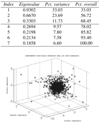
Table 1: Eigenvaluesλiand variance percentages of PCs.
Index Eigenvalue Pct. variance Pct. overall
1 0.9302 33.03 33.03
2 0.6670 23.69 56.72
3 0.3303 11.73 68.45
4 0.2694 9.57 78.02
5 0.2198 7.80 85.82
6 0.2134 7.58 93.40
7 0.1858 6.60 100.00
Figure 3: 3D schematic representation of the three first principal components.
and the more relevant principal components (thus we don’t use the other series directly).
Using a training set consisting of 1000 samples, we com-puted the first 3 principal components. The matrix used consist of the complete set of series (every stock). As we mentioned in Section 3.3.2, we determinate the number of inputs to improve the prediction result of interest using the principal components as additional data input. We remark that the 3 components represents about70%of the overall variance (table 1). In a three dimensional space we can plot the components as is shown in figure 3.
Finally, the last 10 samples of the complete set (1000) were used to compare prediction results with and without exogenous inputs. In addition, in this example we included the well-known sphering or y-score transformation [33](as the variance along all principal components equals one):
wi=
p
λi
−1
·ui , (27)
instead of using the original eigenvector ui. This trans-formation is very common in the field of artificial neural networks and in many ICA-algorithms (whitening) in a pre-processing step as it completely removes all correlations up to the2ndorder.
infor-Figure 4: Prediction results with and without exogenous information using NAPA-PRED. The solid line is the real time series, asterisks (*) are results using NAPA-PRED, and crosses (+) are results using NAPA-PRED+PCA
Table 2: NRMSE for last 10 points (normalized round mean square error).
Mode NRMSE Error
With PCA 0.7192
Without PCA 0.5189
mation extracted using this technique forces redefining the preprocessing step in a few iterations. This is related to the fact that we choose the principal components instead of the original series (5 variables); this choice would in-crease even more the input space dimension reducing the efficiency of the model.
3.4.2 Prediction Results
We compare prediction results obtained using the algorithm in section 2, rejecting the regularization term with and without the method proposed in this Section as is shown in figure 4. Prediction results improve and it is due to frac-tion of exogenous informafrac-tion included. In table 2 we show that (after transformations are inverted) the results for these 10 point are improved in a percentage around7%.
3.5 Conclusions
From the results in the previous Section, itt’s clear that the originally proposed method in [3], improves algorithms ef-ficiency. This increase is based on selecting a suitable input space using a statistic method (PCA) and to date, it’s the only way to develop it.
However the reader can notice the problems of this method. These problems are mentioned in the introduction of the chapter and are about the order of statistics used. In addition the increasing dimensionality (“curse of dimen-sionality”) can cause serious problems (we were using a 5
dimensional input space) damaging the quality of the re-sult. Neural networks are very sensitive to this problem be-cause of the number of neurons to ensure universal approx-imation conditions [39] grows exponentially with the input space dimension unlike multilayer perceptrons, i.e. they are global approximations of nonlinear transformations, so they have a natural capacity of generalization [22, Sec. 7.9] with limited data set.
4 RNs and ICA
In this Section we describe a method for volatile time series forecasting using Independent Component Analysis (ICA) algorithms (see [40]) and Savitzky-Golay filtering as pre-processing tools. The preprocessed data will be introduce in a based radial basis functions (RBF) Artificial Neural Network (ANN) and the prediction result will be compared with the one we get without these preprocessing tools. This method is a generalization of the classical Principal Com-ponent Analysis (PCA) method for exogenous information inclusion (see Section 3)
4.1 Basic ICA
ICA has been used as a solution of the blind source sepa-ration problem [10] denoting the process of taking a set of measured signal in a vector,x, and extracting from them a new set of statistically independent components (ICs) in a vectory. In the basic ICA each component of the vectorx
is a linear instantaneous mixture of independent source sig-nals in a vectorswith some unknown deterministic mixing coefficients:
xi= N
X
i=1
aijsj (28)
Due to the nature of the mixing model we are able to es-timate the original sourcess˜iand the unmixing weightsbij applying i.e. ICA algorithms based on higher order statis-tics such as cumulants.
˜
si= N
X
i=1
bijxj (29)
Using vector-matrix notation and defining a time series vectorx= (x1, . . . , xn)T,s,˜sand the matrixA={aij} andB={bij}we can write the overall process as:
˜s=Bx=BAs=Gs (30)
where we defineGas the overall transfer matrix. The es-timated original sources will be, under some conditions in-cluded in Darmois-Skitovich theorem (chapter 1 in [41]), a permuted and scaled version of the original ones. Thus, in general, it is only possible to findGsuch thatG= PD
This model (equation (28)) can be applied to the stock series where there are some underlying factors like sea-sonal variations or economic events that affect the stock time series simultaneously and can be assumed to be quite independent [42].
4.2 Preprocessing Time Series with
ICA+Filtering
The main goal, in the preprocessing step, is to find non-volatile time series including exogenous information i.e. fi-nancial time series, easier to predict using ANNs based on RBFs. This is due to smoothed nature of thekernel func-tions used in regression over multidimensional domains [43]. We propose the following Preprocessing Steps
– After whitening the set of time series
{xi}ni=1(subtracting the mean of each time
se-ries and removing the second order statistic effect or covariance matrix diagonalization process—see Section 3 for further details)
– We apply an ICA algorithm to estimate the original sourcessiand the mixing matrixAin equation (28). Each IC has information of the stock set weighted by the components of the mixing matrix. In particular, we use an equivariant robust ICA algorithm based in cumulants (see [41] and [6]) however another choices can be taken instead, i.e. in [40]. The unmixing matrix is calculated according the following iteration:
B(n+1)=B(n)+µ(n)(C1,β
s,sSβs −I)B(n) (31)
whereIis the identity matrix,C1,β
s,s is theβ+ 1order cumulant of the sources (we choseβ = 3in simula-tions) ,Sβ
s =diag(sign(diag(Cs1,β,s)))andµ(n)is the step size.
Once convergence, which is related to cross-cumulants 4 absolute value, is reached, we estimate the mixing matrix invertingB.
Generally, the ICs obtained from the stock returns re-veal the following aspects [8]:
1. Only a few ICs contribute to most of the move-ments in the stock return.
2. Large amplitude transients in th dominant ICs contribute to the major level changes. The non-dominant components do not contribute signifi-cantly to level changes.
3. Small amplitude ICs contribute to the change in levels over short time scales, but over the whole period, there is little change in levels.
4Fourth order cumulant between each pair of sources must equals zero.
This is the essential condition of statistical independence as is shown in chapter 3 in [6].
– Filtering.
1. We neglect non-relevant components in the mix-ing matrixAaccording to their absolute value. We consider the rows Ai in matrix Aas vec-tors and calculate the mean Frobenius norm 5 of each one. Only the components bigger than mean Frobenius norm will be considered. This is the principal preprocessing step using PCA tool but in this case this is not enough.
˜
A=Z·A (32) where{Z}ij= [{A}ij > ||Ain||F r]
2. We apply a low band pass filter to the ICs. We choose the well-adapted for data smooth-ing Savitsky-Golay smoothsmooth-ing filter [44] for two reasons: a)ours is a real-time application for which we must process a continuous data stream and wish to output filtered values at the same rate we receive raw data andb)the quantity of data to be processed is so large that we just can afford only a very small number of floating op-erations on each data point thus computational cost in frequency domain for high dimensional data is avoided even the modest-sized FFT (see in [40]). This filter is also called Least-Squares [45] or DISPO [46]. These filters derive from a particular formulation of the data smoothing problem in the time domain and their goal is to find filter coefficientscnin the expression:
¯
si= nR
X
n=−nL
cnsi+n (33)
where{si+n}represent the values for the ICs in a window of length nL+nR+ 1centered on
iand˜siis the filter output (the smoothed ICs), preserving higher moments [47].
For each pointsiwe least-squares fit amorder polynomial for allnL+nR+1points in the mov-ing window and then sets˜i to the value of that polynomial at positioni. As shown in [47] there are a set of coefficients for which equation (33) accomplishes the process of polynomial least-squares fitting inside a moving window:
cn ={(MT ·M)−1(MT ·en)}0=
=Pmj=0{(MT ·M)−1}0
j·nj
where {M}ij = ij, i = −nL, . . . , nR, j =
0, . . . , m, andenis the unit vector with−nL<
n < nR. Note that equation (34) implies that we need only one row of the inverse matrix (numer-ically we can get this by LU decomposition [47], with only a single backsubstitution).
5Givenx∈ Rn, its Frobenius norm is||x|| F r≡
qPn
Figure 5: Schematic representation of prediction and filter-ing process.
– Reconstructing the original series using the smoothed ICs and filteredA˜ matrix we obtain a less high fre-quency variance version of the series including exoge-nous influence of the exogeexoge-nous ones. We can write using equations 42 and 41.
x=A˜·¯s (34)
4.3 Time Series Forecasting Model
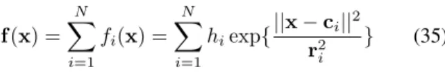
We use an ANN based on RBFs to forecast a seriesxifrom the Stock Exchange building a forecasting functionPwith the help of the algorithm presented in Section 2, for one of the set of signals{x1, . . . , xn}. As shown in Section 2 the individual forecasting function can be expressed in terms of RBFs as [48]:
f(x) =
N
X
i=1
fi(x) = N
X
i=1
hiexp{||x−ci||
2
r2
i
} (35)
wherexis a p-dimensional vector input at timet,Nis the number of neurons (RBFs) ,fi is the output for each neu-ron i-th ,ciis the centers of i-th neuron which controls the situation of local space of this cell andri is the radius of the i-th neuron. The overall output is a linear combination of the individual output for each neuron with the weight of hi. Thus we are using a method for moving beyond the linearity where the core idea is to augment/replace the vector inputx with additional variables, which are trans-formations of x, and then use linear models in this new space of derived input features. RBFs are one of the most popularkernelmethods for regression over the domainRn and consist on fitting a different but simple model at each query pointciusing those observations close to this target point in order to get a smoothed function. This localization is achieved via a weighting function orkernel fi.
The preprocessing step suggested in Section 4.2 is nec-essary due to the dynamics of the series (the algorithm pre-sented Section 2 is sensitive to this preprocessed series) and it will be shown that results improve noticeably [40]. Thus we use as input series the smoothed ones obtained from equation (45).
Figure 6: Set of stock series.
0 200 400 600 800 1000 1200 1400 1600 1800 2000 0
20 40 60 80 100 120
Figure 7: Set of ICs of the stock series.
0 20 40 60 80 100 120 140 160
35 40 45 50 55 60 65 70
0 10 20 30 40 50 60 70 80 44
46 48 50 52 54 56 58 60
Figure 9: Zoom on figure 8.
0 20 40 60 80 100 120 140 160
0 0.5 1 1.5 2 2.5 3 3.5
Figure 10: NRMSE evolution for ANN method and ANN+ICA method for Bankinter Series; theret’s a notice-able improvement even under volatile conditions.
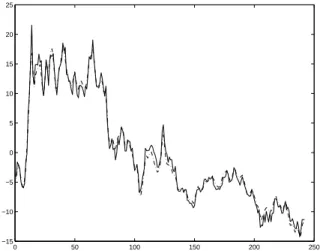
0 50 100 150 200 250
−15 −10 −5 0 5 10 15 20 25
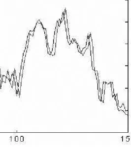
Figure 11: Real series from ICA reconstruction (scaled old version)(line) and preprocessed real series (dotted line). Selected Stock: Bankinter
140 160 180 200 220 240
−15 −10 −5 0 5
Figure 12: Zoom on figure 11.
4.4 Simulations
In the current simulation we have worked with an index of a Spanish bank (Bankinter) and other companies (such as exogenous variables) during the same period to investigate the effectiveness of ICA techniques for financial time series (figure 6). We have specifically focussed on the dowjones from american stock, which we consider the most repre-sentative sample of the american stock movements, using closing prices series.
We considered the closing prices of Bankinter for pre-diction and 10 indexes of intenational companies (IBM, JP Morgan, Matsushita, Oracle, Phillips, Sony, Microsoft, Vo-daphone, Citigroup and Warner). Each time series includes 2000 points corresponding to selling days (quoting days).
We performed ICA on the Stock returns using the ICA algorithm presented in Section 4.2 assuming that the num-ber of stocks equals the numnum-ber of sources supplied to the mixing model. This algorithm whiten the raw data as the first step. The ICs are shown in the figure 7. These ICs rep-resents independent and different underlying factors like seasonal variations or economic events that affect the stock time series simultaneously. Via the rows ofAwe can re-construct the original signals with the help of these ICs i.e. Bankinter stock after we preprocess the raw data:
– Frobenius Filtering: the original mixing matrix6:
A=
. .. ... ... ... ...
. . . 0.33 −0.23 0.17 0.04
. . . −0.28 1.95 −0.33 4.70 . . . 0.33 −0.19 0.05 −0.23
. . . ... ... ... ...
(36)
6We show and select the relevant part of the row corresponding to the
Figure 13: Delay problem in ANNs
is transformed to:
˜ A=
. .. ... ... ... ...
. . . 0.33 −0.23 0.17 0.04
. . . 0 1.95 0 4.70 . . . 0.33 −0.19 0.05 −0.23
. . . ... ... ... ...
(37)
thus we neglect the influence of two ICs on the origi-nal5thstock. Thus only a few ICs contribute to most of the movements in the stock returns and each IC contributes to a level change depending its amplitude transient [8].
– We compute a polynomial fit in the ICs using the li-brary supported byMatLaband the reconstruction of the selected stock (see figure 11) to supply the ANN.
In figures 8 and 9 we show the results (prediction for 150 samples) we obtained using our ANN with the latter ICA method. We can say that prediction is better with the preprocessing step avoiding the disturbing peaks or conver-gence problems in prediction. As is shown in figure 10, the NRMSE is always lower using the techniques we discussed in Section 4.3.
Finally, with these models we avoid the “curse of dimen-sionality” or difficulties associated with the feasibility of density estimation in many dimensions presented in AR or ANNs models (i.e RAN networks without input space con-trol, see Section 2) with high number of inputs as shown in figure 14 and the delay problem presented in non relevant time periods of prediction (bad capacity of generalization in figure 13). In addition, we improve the model presented in Section 3 in two ways:
Figure 14: curse of dimensionality
– This method includes more relevant information (higher order statistics) in which PCA is the first step in the process.
– The way of including extra information avoids “curse of dimensionality” in any case.
4.5 Conclusions
In this Section we showed that prediction results can be im-proved with the help of techniques like ICA. ICA decom-pose a set of 11 returns from the stock into independent components which fall in two categories[40]:
1. Large components responsible of the major changes in level prices and
2. Small fluctuations responsible of undesirable fluctua-tions in time.
Smoothing this components and neglecting the non-relevant ones we can reconstruct a new version of the Stock easier to predict. Moreover we describe a new filtering method to volatile time series that are supplied to ANNs in real-time applications.
5 Multidimensional Regularization
Networks
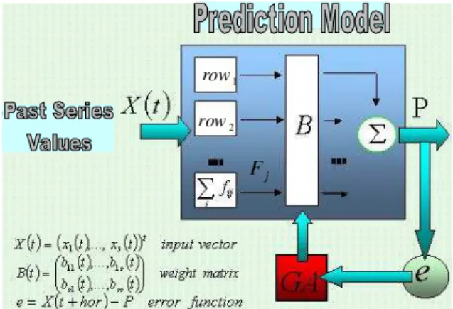
Figure 15: Schematic representation of MRN with adaptive radius, centers and input space ANNs (CPM CrossOver Prediction Model). [5]
5.1 Forecasting Model
The new prediction model is shown in figure 15. We con-sider a data set consisting of some correlated signals from the Stock Exchange and seek to build a forecasting function
P, for one of the sets of signals{series1, . . . , seriesS}, which allows exogenous data from the other series to be included. If we consider just one series (see Section 2) the individual forecasting function can be expressed in terms of RBFs as in [48]:
F(x) =
N
X
i=1
fi(x) = N
X
i=1
hi·exp
½
||x−ci||2
r2
i
¾
(38)
wherexis a p-dimensional vector input at timet,Nis the number of neurons (RBFs) ,fiis the output for eachi−th neuron,ciis the centers of thei−thneuron which controls the situation of local space of this cell andri is the radius of the i-th neuron. The overall output is a linear combina-tion of the individual outputs for each neuron with a weight ofhi. Thus we are using a method for moving beyond lin-earity in which the key idea is to augment/replace the vec-tor input xwith additional variables, which are transfor-mations ofx, and then use linear models in this new space of derived input features. RBFs are one of the most popu-larkernelmethods for regression over the domainRnand consist of fitting a different but simple model at each query pointciusing the observations close to this target point in order to get a smoothed function (see previous Sections). This localization is achieved via a weighting function or
kernelfi.
We apply/extend this regularization concept (see Section 2, to extra series, see figure15, including a row of neurons (equation (38)) for each series, and weight these values by a factorbij. Finally, the overall smoothed function for the stockjis defined as:
Pj(x) = S
X
i=1
bijFi(xi, j) (39)
whereFiis the smoothed function of each series,Sis the number of input series andbij are the weights for j-stock forecasting. Obviously one of these weight factors must be relevant in this linear fit (bjj ∼1, or auto weight factor).
Matrix notation can be used to include the set of fore-casts in an S-dimensional vectorP(Bin figure15):
P(x) =diag(B·F(x)) (40)
whereF= (F1, . . . ,FS)is anS×Smatrix withFi∈ RS andBis anS×S weight matrix. The operatordiag ex-tracts the main diagonal. Because the number of neurons and the input space dimension increases in prediction func-tion (equafunc-tion (40)), we must control them (parsimony) to reduce curse of dimensionality effect and overfitting.
To check this model, we choose a set of values for the weight factors as functions of correlation factors between the series, and thus equation (39) can be expressed (replac-ingPjwithP) as:
P(x) = (1−
S
X
i6=j
ρi)Fj+ S
X
i6=j
ρiFi (41)
wherePis the forecasting function for the desired stockj
andρiis the correlation factor with the exogenous seriesi. We can include equation (41) in the Generalized Addi-tive models for regression proposed in supervised learning [43]:
E{Y|X1, . . . ,Xn}=α+f1(X1) +. . .+fn(Xn) (42)
whereXisusually represent predictors andY represents the system output; fjs are unspecific smooth ("nonpara-metric") functions. Thus we can fit this model by mini-mizing the mean square error function or by other methods presented in [43] (in the next Section we use a GA, a well known optimization tool, to minimize the mean square er-ror).
5.2 Forecasting Model and Genetic
Algorithms
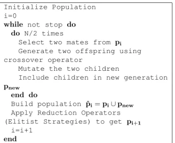
MRN uses a GA for bi parameter fitting. A GA can be modelled by means of atime inhomogeneous Markovchain [49] obtaining interesting properties related to weak and strong ergodicity, convergence and the distribution prob-ability of the process (see [50]). In the latter reference, a canonical GA is constituted by operations of parameter encoding, population initialization, crossover , mutation, mate selection, population replacement, fitness scaling, etc. proving that with these simple operators a GA does not converge to a population containing only optimal members. However, there are GAs that converge to the optimum,The Elitist GA[51] and those which introduceReduction Oper-ators[52].
Table 3: Pseudo-code of GA.
Initialize Population i=0
while not stop do do N/2 times
Select two mates from pi Generate two offspring using crossover operator
Mutate the two children
Include children in new generation
pnew
end do
Build population ˆpi=pi∪pnew Apply Reduction Operators (Elitist Strategies) to get pi+1
i=i+1
end
model on probability distributions (S) over the set of all possible populations of a fixed finite size. LetCthe set of all possible creatures in a given world (vectors of dimen-sion equal to the number of extra series) and a function
f : C → R+. The task of GAs is to find an element c ∈ C for whichf(c)is maximal. We encode creatures into genes and chromosomes or individuals as strings of length`of binary digits (size of AlphabetAisa= 2) using one-complement representation; other encoding methods, also possible i.e [54], [55],[56] or [57], where the value of each parameter is a gene and an individual is encoded by a string of real numbers instead of binary ones.
In the Initial Population Generation step (choosing ran-domlyp∈℘N, where℘N is the set of populations, i.e the set of N-tuples of creatures containingaL≡N·` elements) we assume that creatures lie in a bounded region[0,1](at the edge of this region we can reconstruct the model with-out exogenous data). After the initial populationphas been generated, the fitness of each chromosomeciis determined via the function:
f(ci) = 1
e(ci) (43)
whereeis an error function (i.e square error sum in a set of neural outputs, adjusting the convergence problem in the optimal solution by adding a positive constant to the de-nominator)
The next step in canonical GA is to define the Selection Operator. New generations for mating are selected depend-ing on their fitness function values usdepend-ingroulette wheel se-lection. Letp = (c1, . . . , cN) ∈ ℘N,n ∈ N andf the fitness function acting in each component ofp. Scaled fit-ness selection ofpis a lottery for every position1≤i≤N
in populationpsuch that creaturecjis selected with prob-ability:
fn(p, j)
PN
i=1fn(p, i)
(44)
thus proportional fitness selection can be described by column stochastic matricesFn,n∈ N, with components:
hq,Fnpi= N
Y
i=1
n(qi)fn(p, qi)
PN
j=1fn(p, j)
(45)
wherep, q ∈ ℘N sopi, qi ∈C,h. . .idenotes the stan-dard inner product, andn(di)the number of occurrences of
qiinp.
Once the two individuals have been selected, an elemen-tary crossover operator C(K, Pc) is applied (setting the crossover rate at a value, i.e. Pc →0, which implies chil-dren similar to parent individuals) that is given (assuming
N even) by:
C(K, Pc) = N/Y2
i=1
((1−Pc)I+PcC(2i−1,2i, ki)) (46)
whereC(2i−1,2i, ki)denotes elementary crossover op-eration of ci, cj creatures at position 1 ≤ k ≤ ` andI the identity matrix, to generate two offspring (see [50] for details of the crossover operator).
The Mutation OperatorMPm is applied (with
probabil-ityPm) independently at each bit in a populationp∈℘N, to avoid premature convergence (see [54] for further dis-cussion). The multi-bit mutation operator with change probability following a simulated annealing law with re-spect to the position1≤i≤Linp∈℘N:
Pm(i) =µ·exp
Ã
−mod{i−1
N }
∅
!
(47)
where∅is a normalization constant andµthe change prob-ability at the beginning of each creaturepiin populationp; can be described as a positive stochastic matrix in the form:
hq,MPmpi=µ
∆(p,q)exp³−P∆(p,q)
dif(i)
mod{i−1 N }
∅
´
·QLequ−∆((i)p,q)h1−µ·exp³−mod{i−N1}
∅
´i
(48) where∆(p, q)is the Hamming distance betweenpand
q∈ ℘N,dif(i)resp. equ(i)is the set of indexes where p andqare different resp. equal. Following from equation (48) and checking how the matrices act on populations we can write:
MPm = N
Y
λ=1
¡
[1−Pm(λ)]1+Pm(λ)mˆ1(λ)
¢
(49)
where mˆ1(λ) = 1⊗1. . .⊗
λ
z}|{
ˆ
m1 ⊗. . . ⊗1 is a linear
linear 1-bit mutation operator onV1, the free vector space overA. The latter operator is defined acting on Alphabet as:
hˆa(τ0),mˆ1ˆa(τ)i= (a−1)−1, 0≤τ0 6=τ ≤a−1 (50)
i.e. probability of change a letter in the Alphabet once mu-tation occurs with probability equal toLµ.
The spectrum ofMPmcan be evaluated according to the
following expression:
sp(MPm) = (µ
1− µ(λ) a−1
¶λ
; λ∈[0, L]
)
(51)
whereµ(λ) = exp³−mod{λ−N1}
∅
´
.
The operator presented in equation (49) has similar prop-erties to the Constant Multiple-bit mutation operatorMµ.
Mµis a contracting map in the sense presented in [53]. It is easy to prove that MPm is a another contracting map,
using the Corollary B.1 in [6] and the eigenvalues of this operator(equation (51)).
We can also compare the coefficients of ergodicity:
τr(MPm)< τr(Mµ) (52)
where τr(X) = max{kXvkr : v ∈
Rn, v⊥e and kvk r= 1}.
Mutation is more likely at the beginning of the string of binary digits ("small neighborhood philosophy"). In order to improve the speed convergence of the algorithm we have included mechanisms such as elitist strategy (reduction op-erator [58]) in which the best individual in the current gen-eration always survives into the next (a further discussion about reduction operator,PR, can be found in [59]).
Finally the GA is modelled, at each step, as the stochas-tic matrix product acting on probability distributions over populations:
SPn
m,Pnc =P n
R·Fn·CkPn
c ·MPnm (53)
The GA used in forecasting function (equation (39)) has absolute error value start criterion (i.e error > uga = 1.5). Once it starts, it uses the values (or individual) found to be optimal (elite) the last time, and applies lo-cal search (using the selected mutation and crossover op-erators) around this elite individual. Thus we perform an efficient search around an individual (set ofbis) in which one parameter is more relevant than the others.
The computational time depends on the encoding length, number of individuals and genes. Because of the prob-abilistic nature of the GA- based method, the proposed method almost converges to a global optimal solution on average. In our simulation nonconvergent case was found. Table 3 shows the GA-pseudocode and in [5] the iterative procedure implemented for the overall prediction system including GA is shown.
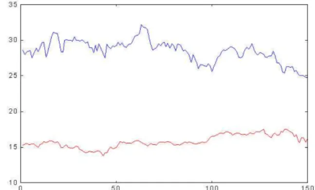
Figure 16: Set of data series. Top: Real Series ACS;Bottom: Real Series BBVA.
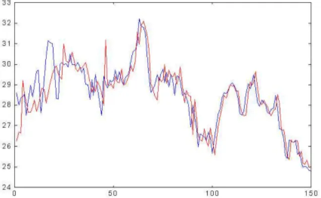
Figure 17: Real Series and Predicted ACS Series with MRN.
Figure 18: Absolute Error Value with MRN.
Figure 20: Absolute Error Value with MRN + GA.
Figure 21: Real Series and Predicted ACS Series without exogenous data.
5.3 Simulations and Conclusions.
With the aim of assessing the performance of the MRN we have worked with indexes of different Spanish banks and other companies during the same period. We have specif-ically focussed on the IBEX35 index of Spanish stock, which we consider the most representative sample of Span-ish stock movements. We usedMatLabto implement MRN on a Pentium III at 850MHz.
We started by considering the most simplest case, which consists of two time series corresponding to the compa-nies ACS (series1) and BBVA (series2). The first one is the target of the forecasting process; the second one is introduced as external information. The period under study covers the year 2000. Each time series includes 200 points corresponding to selling days (quoting days).
We highlight two parameters in the simulation process. The horizon of the forecasting process (hor) was set at1; the weight function of the forecasting function was a corre-lation function between the two time series for theseries2
(in particular we chose its square) and the difference to one for the series 1. We took a forecasting window (W) of 10 lags, and the maximum lag number was set at double the value of W, and thus we built a10×20Toeplitz matrix. We started at time pointto = 50. Figures 17,18 19 and 20 show the forecasting results from lag 50 to lag 200 corre-sponding toseries1.
Note the instability of the system in the very first
itera-Figure 22: NRMSE evolution for MRN(dot) MRN + GA(line).
Figure 23: Set of series for complete simulation.
Figure 25: NRMSE evolution using ICA method and MRN.
Table 4: Correlation coefficients between real signal and the predicted signal for different lags.
delay ρ delay ρ
0 0.89 0 0.89
+1 0.79 -1 0.88
+2 0.73 -2 0.88
+3 0.68 -3 0.82
+4 0.63 -4 0.76
+5 0.59 -5 0.71
+6 0.55 -6 0.66
+7 0.49 -7 0.63
+8 0.45 -8 0.61
+9 0.45 -9 0.58
+10 0.44 -10 0.51
Table 5: Dynamics and values of the weights for the GA.
bseries T1 T2 T3 T4
b1 0.8924 0.8846 0.8723 0.8760
b2 0.2770 0.2359 0.2860 0.2634
tions until it reaches an acceptable convergence. The most interesting feature of the result is shown in table 4; from this table it is easy to deduce that if we move one of the two series horizontally the correlation between them dra-matically decreases. This proves that we avoid the delay problem (trivial prediction) shown by certain networks (see figure 21), in periods where the information introduced to the system is non-relevant. This is due to the increase of in-formation (series2) associated with an increase in neuron resources. At the end of the process we used20neurons for net 1 and21for net 2. Although forecasting function is acceptable we would expect a better performance with bigger data set.
The next step consists of using the complete algorithm including the GA. A population of 40individuals (Nind) was used, with a2×1dimension; we used this small num-ber because we had a bounded searching space and we were using a single PC. The genetic algorithm was run four times before reaching the convergence (when the error increase by1.5points, see error plot in figure 20 to see the effect of GA) ; the individuals were codified with34bits (17bits for each parameter). In this case convergence is defined in terms of the adjustment function; other authors use other parameters of the GA, like the absence of change in the individuals after a certain number of generations, etc. We observed a considerable improvement in the forecasting re-sults and noted disappearance of the delay problem, as is shown in table 4. This table represents the correlation be-tween the real function and the neural function for different lags. The correlation function presents a maximum at lag
0.
The number of neurons at the end of the process is the same as in the latter case, because we have only modified the weight of each series during the forecasting process. The dynamics and values of the weights are shown in table 5.
Error behaviour is shown in figures. Note:
– We can bound the error by means of a suitable selec-tion of the parameters bi, when the dynamics of the series is coherent (avoiding large fluctuations in the stock).
– The algorithm converges faster, as is shown at the very beginning of the graph.
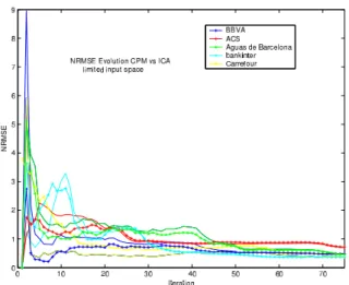
Finally we carried out a simulation with 9 indexes and computed the prediction function for 5 series, obtaining similar results, as presented in figure 24. In the complete model we limited the input space dimension to3for extra series and5for target series (figure 22). NRMSE depends on each series (data set) and target series (evolution). In figure 25 we also compare the ICA method versus MRN for limited data set (70 iterations). NRMSE of indexes increases at the beginning of the process using the ICA method and converges to CPM NRMSE values when the data set increases (estimators approach higher order statis-tics). This effect is also observed when the dynamics of the series change suddenly due to a new independent event.
Due to the symmetric character of our forecasting model, it is sufficient to implement it in parallel programming soft-ware (such as PVM —Parallel Virtual Machine—) or MPI —Message-Passing Interface— [60]) to build a more gen-eral forecasting model for the complete set of series. We would spawn the same number for offspring processes and banks; these process would run forecasting vectors, which would be weighted by a square matrix with dimension equal to the number of series B. The “master” process would have the results of the forecasting process for the calculus of the error vector, in order to update the neuron resources. Thus we would take advantage of the computa-tional cost of a forecasting function to calculate the rest of the series (see [60]).
5.3.1 Conclusions
This new forecasting model for time-series is characterized by:
– The enclosing of external information. We avoid pre-processing and data contamination applying by ICA and PCA for limited data sets or sudden new shocks. These techniques can be included in MRN under bet-ter conditions. Series are introduced into the net di-rectly.
– The forecasting results are improved using hybrid techniques like GA.
– The possibility of implementing in parallel program-ming languages (i.e. PVM — see [60]); and the improved performance and lower computational time achieved using a parallel neural network.
6 Comparison among methods
Consider the set of series in Figure 6, using 1000 point as training samples. We apply the latter models to fore-cast Sony index in 70 future points using the other indexes as endogenous variables. Following the methodology de-scribed in the previous sections we get:
– PCA operation: in this case results using PCA are not so good as we expected. The volatile nature of the
Table 6: Eigenvaluesλiand variance percentages of PCs.
Index Eigenvalue Pct. variance Pct. overall
1 0.0031 35.1642 35.1642
2 0.0016 17.9489 53.1131
3 0.0010 11.7188 64.8319
4 0.0006 6.9857 71.8176
5 0.0005 5.7787 77.5963
6 0.0004 4.8978 82.4941
7 0.0004 4.4184 86.9125
8 0.0004 4.2492 91.1617
9 0.0003 3.7238 94.8855
10 0.0003 3.2031 98.0886
11 0.0002 1.9113 100.00
0 100 200 300 400 500 600 700 800 900 1000 −0.4
−0.3 −0.2 −0.1 0 0.1 0.2 0.3
Figure 26: Closing prices evolution for selected indexes (Figure 6), after logarithmic transformation and differenti-ation.
series and the lack of information from the 3 princi-pal components used contributes to this failure. The 3 components only hold a fraction equal to 64% of vari-ance as is shown in Table 6, however if we increase the number of components used in prediction we get worse results owing to “curse of dimensionality”.
– MRN operation: MRN get good prediction results comparing with PCA method, however in the last iterations PCA and MRN methods are of similar NRMSE. The main disadvantages of MRN are com-putational demand and the need for bounding input space dimension.
0 100 200 300 400 500 600 700 800 900 1000 −5
0 5 10 15 20 25 30
Figure 27: ICA ICs for the set of indexes.
0 10 20 30 40 50 60 70
0 0.5 1 1.5 2 2.5 3
NRMSE SONY
ANN+ICA ANN+PCA CPM
Figure 28: NRMSE evolution of SONY index for the 70 forecasted points using exogenous methods.
Acknowledgement
We want to thank SESIBON and HIWIRE grants from Spanish Government for funding.
References
[1] G. Box, G. Jenkins, and G. Reinsel, Time Series Analysis: Forecasting and Control, 3rd ed. Prentice-Hall. Englewood Cliffs, New Jersey, U.S.A., 1994.
[2] J. Platt, “A resource-allocating network for function interpolation,”Neural Computation, vol. 3, pp. 213– 225, 1991.
[3] M. Salmerón, J. Ortega, C. Puntonet, and F. Pelayo,
Time Series Prediction with Hybrid Neuronal, Statis-tical and Matrix Methods (in Spanish). Department of Computer Architecture and Computer Technology. University of Granada, Spain, 2001.
[4] M. Salmerón, J. Ortega, C. G. Puntonet, and A. Pri-eto, “Improved ran sequential prediction using or-thogonal techniques,” Neurocomputing, vol. 41, pp. 153–172, 2001.
[5] J. M. Górriz, C. G. Puntonet, M. Salmerón, and J. González, “New model for time-series forecasting using rbf´s and exogenous data,”Neural Computation and Applications, Vol 13 Issue 2. Jun. 2004., 2003.
[6] J. M. Górriz, “Algoritmos híbridos para la mod-elización de series temporales con técnicas ar-ica,” Ph.D. dissertation, University of Cádiz , Departa-mento de Ing. de Sistemas y Aut. Tec. Electrónica y Electrónica. http://wwwlib.umi.com/cr/uca/main, 2003.
[7] T. Masters,Neural, Novel and Hybrid Algorithms for Time Series Prediction. John Wiley & Sons. New York, U.S.A., 1995.
[8] A. Back and A. Weigend, “Discovering structure in fi-nance using independent component analysis,” Com-putational Finance, 1997.
[9] A. Back and T. Trappenberg, “Selecting inputs for modelling using normalized higher order statistics and independent component analysis,” IEEE Trans-actions on Neural Networks, vol. 12, 2001.
[10] A. Hyvarinen and E. Oja, “Independent component analysis: Algorithms and applications,”Neural Net-works, vol. 13, pp. 411–430, 2000.