A Background on programming
language and program verification
Programs We assume given a set of function sym-bols with their arity. For simplicity, we consider the case where operators are untyped and have arity 0 (con-stants), 1 (unary functions), and 2 (binary functions). We letc,c1, andc2 range over constants, unary func-tions and binary funcfunc-tions respectively. Expressions are built from function symbols and variables. The set of expressions is defined inductively by the following grammar:e ::= x variable
| c constant
| c1(e) unary function | c2(e1, e2) binary function
We next assume given a set of atomic predicates. For simplicity, we also consider that predicates have arity 1 or 2, and letP1 andP2 range over unary and binary predicates respectively. We define guards using the following grammar:
b ::= P1(e) unary predicate | P2(e1, e2) binary predicate | b1&b2 conjunction | b1||b2 disjunction
| ¬b negation
We next define commands. These include assignments, conditionals, bounded loops and return expressions. The set of commands is defined inductively by the following grammar:
c ::= skip no-op
| x:=e assignment
| c1;c2 sequential composition | if b thenc1elsec2 conditionals
| for(i= 1, . . . , n)do c for loop
| returne return statement
We assume that programs satisfy a well-formedness condition. The condition requires that return ex-pressions have no successor instruction, i.e. we do not allow commands of the form return e; c or if bthen c; returneelsec0;c00. This is without loss of generally, since commands can always be transformed into functionally equivalent programs which satisfy the well-formedness condition.
Single assignment form Our first step to construct characteristic formulae is to transform programs in an intermediate form that is closer to logic. Without loss of generality, we consider loop-free commands, since loops can be fully unrolled. The intermediate form is called a variant of the well-known SSA form [Rosen et al., 1988,
Cytron et al., 1991] from compiler optimization. Con-cretely, we transform programs into some weak form of single assignment. This form requires that every non-input variable is defined before being used, and assigned at most once during execution for any fixed input. The main difference with SSA form is that we do not use so-called -nodes, as we require that variables are assigned at most once for any fixed input. More technically, our transformation can be seen as a compo-sition of SSA transform with a naive de-SSA transform where -nodes are transformed into assignments in the branches of the conditionals.
Path formulae and characteristic formulae Our second step is to define the set of path formulae. Infor-mally, a path formula represents a possible execution of the program. Fix a distinguished variableyfor return values. Then the path formulae of a command c is defined inductively by the clauses:
PFz:=e(y) ={z=e}
PFc1;c2(y) ={ 1^ 2| 12PFc1(y)^ 22PFc2(y)} PFif bthenc1 elsec2(y) ={b^ 1| 12PFc1(y)} [ {¬b^ 2| 22PFc2(y)} PFreturne(y) ={y=e}
The characteristic formula c of a commandcis then
defined as: _
2PFc(y)
One can prove that for every inputs x1, . . . , xn, the formula y(x1, . . . , xn, v) is valid iffthe execution of c on inputs x1, . . . , xn returnsv. Note that, strictly speaking, the formula y contains as free variables the distinguished variabley, the inputsx1, . . . , xn of the program,and all the program variables, sayz1. . . zm. However, the latter are fully defined by the characteris-tic formula so validity of y(x1, . . . , xn, v)is equivalent to validity of9z1. . . zm. y(x1, . . . , xn, v).
B Experiment Details
In this section we provide further details on the detasets and methods used in or experiments, together with some additional results.
B.1 Model Selection
To demonstrate the flexibility of our approach, we explored four different differentiable and non-differentiable model classes, i.e., decision tree, ran-dom forest, logistic regression and multilayer percep-tron (MLP). As the main focus of our work is to generate counterfactuals for a broad range of already trained models, we opted for models’ parametrization that result in good performance on the considered datasets (e.g., default parameters). For instance, for the MLP, we opted for two hidden layers with 10 neu-rons, since it present better performance in the Adult dataset (%82.52/%81.94training/test accuracy) than other architectures with hidden={100}(default)and hidden = {100,100} which result in %81.69/%81.06 and%81.51/%80.82training/test accuracy, respectively. We leave the exploration of other datasets (larger fea-ture spaces), more complex models (deeper MLPs) and other SMT solvers as future work.
B.2 Datasets
Here we detail the different types of variables present in each dataset. We used the default features for the Adult and COMPAS datasets, and applied the same preprocessing used in [Ustun et al., 2019] for the Credit dataset. All samples with missing data were dropped. We remark that we have relied on broadly studied datasets in the literature on fair-ness and interpretability of ML for consequential de-cision making. For instance, the Credit dataset [34] (n= 29,623, d= 14) has been previously studied by the Actionable Recourse work [29], and the Adult [1] (n= 45,222, d = 12, d(one-hot)= 51) and COMPAS [18] (n= 5,278, d= 5, d(one-hot)= 7) have been pre-viously used in the context of fairness in ML [Joseph et al., 2016; Zafar et al., 2017; Agarwal et al. 2018].
Adult(n= 45,222, d= 12, d(one-hot)= 51):
• Integer: Age, Education Number, Hours Per Week • Real: Capital Gain, Capital Loss
• Categorical: Sex, Native Country, Work Class, Marital Status, Occupation, Relationship
• Ordinal: Education Level
Credit(n= 29,623, d= 14, d(one-hot)= 20):
• Integer: Total Overdue Counts, Total Months Overdue, Months With Zero Balance Over Last 6 Months, Months With Low Spending Over Last 6 Months, Months With High Spending Over Last 6 Months
• Real: Max Bill Amount Over Last 6 Months, Max Payment Amount Over Last 6 Months, Most Re-cent Bill Amount, Most ReRe-cent Payment Amount • Categorical: Is Male, Is Married, Has History Of
Overdue Payments
• Ordinal: Age Group, Education Level
COMPAS(n= 5,278, d= 5, d(one-hot)= 7): • Integer:
-• Real: Priors Count
• Categorical: Race, Sex, Charge Degreee • Ordinal: Age Group
B.3 Handling Mixed Data Types
While the proposed approach (MACE) naturally han-dles mixed data types, other approaches do not. Specif-ically, the Feature Tweaking method generates counter-factual explanations for Random Forest models trained on non-hot embeddings of the dataset, meaning that the resulting counterfactuals will not have multiple cat-egories of the same variable activated at the same time. However, because this method is only restricted to working with real-valued variables, the resulting coun-terfactual is must undergo a post-processing step to en-sure integer-, categorical-, and ordinal-based variables are plausible in the counterfactual. The Actionable Re-course method, on the other hand, explanations for Lo-gistic Regression models trained on one-hot embeddings of the dataset, hence requiring additional constraints to ensure that multiple categories of a categorical variable are not simultaneously activated in the counterfactual. While the authors suggest how this can be supported using their method, their open-source implementation converts categorical columns to binary where possible and drops other more complicated categorical columns, postponing to future work. Furthermore, the authors state thatthe question of mutually exclusive features will be revisited in later releases9. Moreover, ordinal variables are not supported using this method. The overcome these shortcomings, the counterfactuals gen-erated by both approaches is post-processed to ensure correctness of variable types by rounding integer-based variables, and taking the maximally activated category as the counterfactual category.
9https://github.com/ustunb/actionable-recourse/ blob/master/examples/ex_01_quickstart.ipynb
C Additional Results
C.1 Comprehensive Distance Results
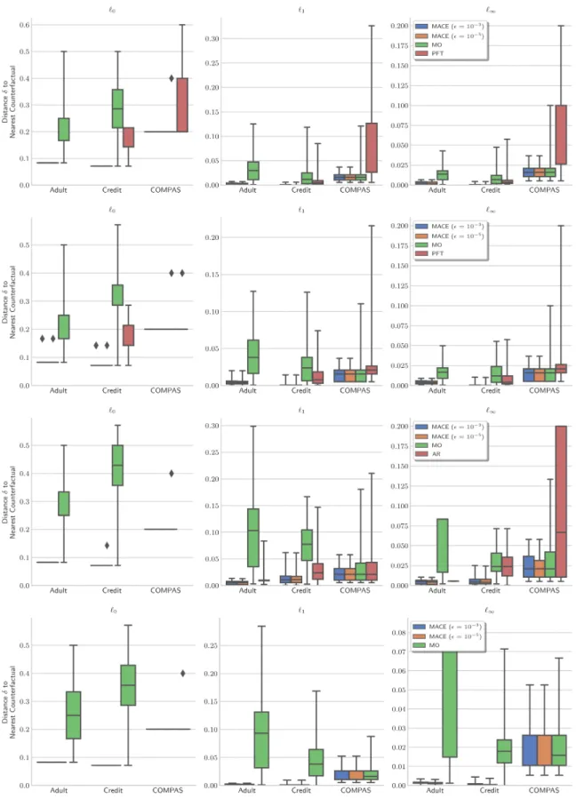
Following the presentation of coverage ⌦ results in Table 2 and relative distance improvement (reduction) in Table 3 of the main body, in Figure 4 we present the complete distribution of counterfactual distances upon termination of Algorithm 1. Importantly, we see that in all setups (approaches⇥models ⇥norms ⇥ datasets), MACE results are at least as good as any other approach (MO, PFT, AR).
C.2 Quality vs Complexity
In the main text and in the previous section, we con-sidered distance comparisonsupon termination of Al-gorithm 1; in this section we explore the effect of the accuracy parameter✏ jointly on quality (distance )
and complexity (run-time⌧)during execution of
Algo-rithm 1. Importantly, the number of calls made to the SATsolver followsO(log(1/✏)), where✏is the desired the accuracy term, i.e., orders of magnitude more accu-racy only cost linearly moreSATcalls. The run-time of each call to theSATsolver is governed by a number of parameters, including the implementation details of the SATsolver10, the compute hardware11, among other factors. Clearly, a higher desired accuracy (i.e.,✏!0) will result in closer counterfactuals ( 2[ ⇤, ⇤+✏]) at the cost of higher run-time (higher⌧), while leaving the
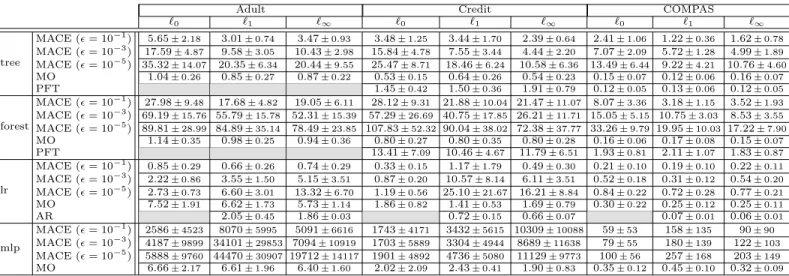
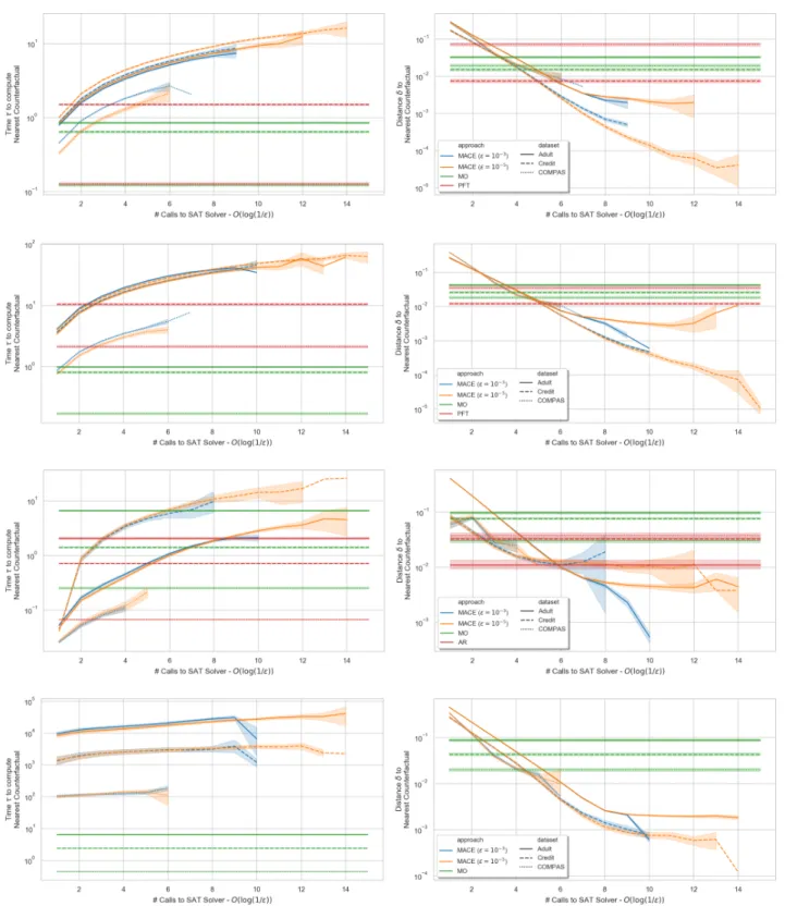
coverage⌦unchanged (remaining at 100%, by design). Figure 5 depicts the average counterfactual distance and average run-time against the number of calls to the SAT solver, confirming the intuition above: not only does MACE always achieve a lower counterfactual distance12 upon termination, in many cases an early termination of MACE generates closer counterfactuals while also being less computationally demanding. In addition to studying the quality vs complexity trade-off against number of calls to the SAT solver, in Ta-ble 6 we compare final run-times (in seconds) upon-termination of Algorithm 1 for various setups. The results show that MACE takes less than 5 seconds for lo-gistic regression; between 5 and 60 seconds for decision trees and random forests; and between one minute and three hours for the multilayer perceptron (outliers were not excluded in computed mean runtimes). In contrast, 10This is assumed beyond the scope of the pa-per; we built MACE atop the open-source PySMT library [Gario and Micheli, 2015] with the Z3 [de Moura and Bjørner, 2008] backend to demonstrate its model-agnostic support of off-the-shelf models.
11All tests were conducted using one X86_64 Xeon(R) CPU @ 2.60GHz, and 8GB memory.
12Reminder: lower distance is more desirable, as it speci-fies the least change required of the individual’s features.
competing approaches (MO, PFT, AR) require at most 30 seconds to generate a counterfactual explanation, when possible (note that the coverage for AR and PFT is often significantly below 100%, and only MACE is able togenerate counterfactuals for the multilayer per-ceptron; MO requires access to the training data as it searches through the training set for a counterfactual). We believe that this difference is compensated (at least for the decision tree, the random forest, and the logistic regression classifiers) by the main properties of MACE compared to previous works, i.e.: i) model-agnostic ({non-}linear, {non-}differentiable, {non-}convex); ii) data-agnostic (heterogeneous features); iii) provable closeness guarantees; and iv) 100% coverage, even under plausibility and diversity constraints. Regard-ing the results on MLPs, we are well aware of prior work that develops efficient SMT-based methods for verifying large deep neural networks (see formal veri-fication of deep neural networks [Huang et al., 2017, Katz et al., 2017, Singh et al., 2019] and optimiza-tion modulo theories [Nieuwenhuis and Oliveras, 2006, Sebastiani and Tomasi, 2012]); indeed we plan to lever-age state-of-the-art tools to improve the efficiency of our implementation, in particular for MLP-based models. With the current implementation of MACE, our main goal was to explore the use of off-the-shelf SMT-solvers already available in Python to generate counterfactu-als in a broad range of settings, justifying our lesser emphasis on efficiency.
In practice the choice of epsilon should reflect the de-sired distance granularity from the operator, the num-ber and range of attributes in the data space, and the decided upon distance norm. For example, using the`0 norm, which tracks the number of attributes changed, the lowest achievable distance granularity is1/J where J is the data dimensionality. Therefore, choosing any
✏<1/Jis sufficient and will result in the optimal coun-terfactual for this choice of distance metric. As another example, for the continuous`1 norm, too much gran-ularity may result in a lack of trust for the end-user – consider the adult dataset with account balance feature with rangeR = $50,000; choosing a fine granularity may result in a counterfactual that suggests that only a few dollars change in the account balance can flip the prediction (e.g., result in the approval of a loan). It is important to point out that this phenomenon is not a fault of the counterfactual generating method (i.e., MACE), but of the robustness of the underlying classifier and its decision boundary. While such an explanation may not be favorable for an end-user, it may assist a system administrator or model designer to assay the robustness and safety of their model prior to deployement.
Table 6: Wall-clock time (seconds) for computing the nearest counterfactual explanation (without constraints). N =⌦MACE\⌦Other factual samples; cells are shaded for unsupported tests. Lower run-time is better. The run-time for MACE depends onO(log(1/✏)), i.e., orders of magnitude more accuracy only cost linearly more run-time. These results should be considered along Tables 2, 3 comparing coverage⌦and distance .
Adult Credit COMPAS
`0 `1 `1 `0 `1 `1 `0 `1 `1 tree MACE (✏= 10 1) 5.65 ±2.18 3.01±0.74 3.47±0.93 3.48±1.25 3.44±1.70 2.39±0.64 2.41±1.06 1.22±0.36 1.62±0.78 MACE (✏= 10 3) 17.59 ±4.87 9.58±3.05 10.43±2.98 15.84±4.78 7.55±3.44 4.44±2.20 7.07±2.09 5.72±1.28 4.99±1.89 MACE (✏= 10 5) 35.32 ±14.07 20.35±6.34 20.44±9.55 25.47±8.71 18.46±6.24 10.58±6.36 13.49±6.44 9.22±4.21 10.76±4.60 MO 1.04±0.26 0.85±0.27 0.87±0.22 0.53±0.15 0.64±0.26 0.54±0.23 0.15±0.07 0.12±0.06 0.16±0.07 PFT 1.45±0.42 1.50±0.36 1.91±0.79 0.12±0.05 0.13±0.06 0.12±0.05 forest MACE (✏= 10 1) 27.98±9.48 17.68±4.82 19.05±6.11 28.12±9.31 21.88±10.04 21.47±11.07 8.07±3.36 3.18±1.15 3.52±1.93 MACE (✏= 10 3) 69.19±15.76 55.79±15.78 52.31±15.39 57.29±26.69 40.75±17.85 26.21±11.71 15.05±5.15 10.75±3.03 8.53±3.55 MACE (✏= 10 5) 89.81 ±28.99 84.89±35.14 78.49±23.85 107.83±52.32 90.04±38.02 72.38±37.77 33.26±9.79 19.95±10.03 17.22±7.90 MO 1.14±0.35 0.98±0.25 0.94±0.36 0.80±0.27 0.80±0.35 0.80±0.28 0.16±0.06 0.17±0.08 0.15±0.07 PFT 13.41±7.09 10.46±4.67 11.79±6.51 1.93±0.81 2.11±1.07 1.83±0.87 lr MACE (✏= 10 1) 0.85 ±0.29 0.66±0.26 0.74±0.29 0.33±0.15 1.17±1.79 0.49±0.30 0.21±0.10 0.19±0.10 0.22±0.11 MACE (✏= 10 3) 2.22 ±0.86 3.55±1.50 5.15±3.51 0.87±0.20 10.57±8.14 6.11±3.51 0.52±0.18 0.31±0.12 0.54±0.20 MACE (✏= 10 5) 2.73±0.73 6.60±3.01 13.32±6.70 1.19±0.56 25.10±21.67 16.21±8.84 0.84±0.22 0.72±0.28 0.77±0.21 MO 7.52±1.91 6.62±1.73 5.73±1.14 1.86±0.82 1.41±0.53 1.69±0.79 0.30±0.22 0.25±0.12 0.25±0.11 AR 2.05±0.45 1.86±0.03 0.72±0.15 0.66±0.07 0.07±0.01 0.06±0.01 mlp MACE (✏= 10 1) 2586 ±4523 8070±5995 5091±6616 1743±4171 3432±5615 10309±10088 59±53 158±135 90±90 MACE (✏= 10 3) 4187 ±9899 34101±29853 7094±10919 1703±5889 3304±4944 8689±11638 79±55 180±139 122±103 MACE (✏= 10 5) 5888 ±9760 44470±30907 19712±14117 1901±4892 4736±5080 11129±9773 100±56 257±168 203±149 MO 6.66±2.17 6.61±1.96 6.40±1.60 2.02±2.09 2.43±0.41 1.90±0.83 0.35±0.12 0.45±0.10 0.32±0.09
Table 7: Percentage of factual samples for which the nearest counterfactual sample requires a reduction in age for a random forest trained on the Adult dataset, and the corresponding increase in distance to nearest counterfactual when restricting the approaches not to reduce age: 100⇥E[ restr./ unrestr. 1].
`0 `1 `1
%age-red. rel. dist. increase %age-red. rel. dist. increase %age-red. rel. dist. increase
MACE (✏= 10 5) 3.6% 0% 7.4% 61.3% 34.2% 13.9%
MO 24.6% 29.7% 34.6% 94.6% 34.2% 66.6%
C.3 Additional Constrained Results
Following the study of counterfactuals that change or reduce age (Section 5), we regenerate counterfactual explanations for those samples for which age-reduction was required, with an additional plausibility constraint ensuring that the age shall not decrease. The results presented in Table 7 show interesting results. Once again, we observe that the additional plausibility con-straint for the age incurs significant increases in the dis-tance of the nearest counterfactual – being, as expected, more pronounced for the`1and the`1norms. For the
`0norm, we find that for the 18 factual samples (i.e., 3.6%⇥500) for which the unrestricted MACE required age-reduction, the addition of the no-age-reduction constraint results in counterfactuals at the same dis-tance, while suggesting a change in work class (5/18) or education level (4/18) instead of changing age.
C.4 Details on diverse counterfactuals example
In the main body, we described a scenario where a logistic regression model had predicted that a loan borrower, John, would default on his loan. Here is
john’s complete feature list: John is a married male between 40-59 years of age with some university degree. Over the last 6 months, Max Bill Amount = 500.0, Max Payment Amount = 60.0, Months With Zero Balance = 0.0, Months With Low Spending = 0.0, Months With High Spending = 1.0. Furthermore, John has a history of overdue payments, his Most Recent Bill Amount = 370.0, and his Most Recent Payment Amount = 40.0
Figure 4: Comparison of approaches for generating unconstrained counterfactual explanations for a(top to bottom) trained decision tree, random forest, logistic regression, and multilayer perceptron model. Here the distribution of distance is shownupon termination of Algorithm 1; lower distance is better. For each bar,N = 500⇥⌦from Table 2, and absent bars refer to ⌦= 0. In all setups, MACE results are at least as good as any other approach.
Figure 5: Comparison of approaches for generating unconstrained counterfactual explanations for a(top to bottom) trained decision tree, random forest, logistic regression, and multilayer perceptron model. Here the average distance and run-time⌧ is shownduring execution of Algorithm 1 (i.e., over number of calls
to theSATsolver); lower distance and lower run-time is better. Other approaches (MO, PFT, AR) would only be shown as a single point on these plots, and therefore we repeat their results over all values of the x-axis for ease of comparison against MACE. Results are averaged over all plausible counterfactuals (N = 500⇥⌦from Table
2,). As expected, Algorithm 1 terminates after different number of iterations depending on the factual instance; this explains the observed larger variance in results for higher number of iterations. These results confirm our intuition: not only does MACE always achieve a lower counterfactual distance upon termination, in many cases an early termination of MACE generates closer counterfactuals while also being less computationally demanding.