How to Discount Cashf lows with Time-Varying
Expected Returns
ANDREW ANG and JUN LIU∗
ABSTRACT
While many studies document that the market risk premium is predictable and that betas are not constant, the dividend discount model ignores time-varying risk pre-miums and betas. We develop a model to consistently value cashf lows with changing risk-free rates, predictable risk premiums, and conditional betas in the context of a conditional CAPM. Practical valuation is accomplished with an analytic term struc-ture of discount rates, with different discount rates applied to expected cashf lows at different horizons. Using constant discount rates can produce large misvaluations, which, in portfolio data, are mostly driven at short horizons by market risk premiums and at long horizons by time variation in risk-free rates and factor loadings.
TO DETERMINE AN APPROPRIATE DISCOUNT RATE for valuing cashf lows, a manager
is confronted by three major problems: the market risk premium must be esti-mated, an appropriate risk-free rate must be chosen, and the beta of the project or company must be determined. All three of these inputs into a standard CAPM are not constant. Furthermore, cashf lows may covary with the risk premium, betas, or other predictive state variables. A standard Dividend Discount Model (DDM) cannot handle dynamic betas, risk premiums, or risk-free rates because in this valuation method, future expected cashf lows are valued at constant discount rates.
In this paper, we present an analytical methodology for valuing stochastic cashf lows that are correlated with risk premiums, risk-free rates, and time-varying betas. All these effects are important. First, the market risk premium is not constant. Fama and French (2002) argue that the risk premium moved to around 2% at the turn of the century from 7% to 8% 20 years earlier. Jagannathan, McGratten, and Scherbina (2001) also argue that the market ex ante risk premium is time varying and fell during the late 1990s. Further-more, a large literature claims that a number of predictor variables, including
∗Ang is with Columbia University and NBER. Jun Liu is at UCLA. We would like to
thank Michael Brandt, Michael Brennan, Bob Dittmar, John Graham, Bruce Grundy, Ravi Jagannathan, and seminar participants at the Australian Graduate School of Management, Columbia University, the Board of Governors of the Federal Reserve, and Melbourne Business School for comments. We also thank Geert Bekaert and Zhenyu Wang for helpful suggestions and especially thank Yuhang Xing for constructing some of the data. We also thank Rick Green (the former editor), and we are grateful to an anonymous referee for helpful comments that greatly improved the paper. The authors acknowledge funding from an INQUIRE UK grant. This paper represents the views of the authors and not of INQUIRE. All errors are our own.
dividend yields (Campbell and Shiller (1988a, b)), risk-free rates (Fama and Schwert (1977)), term spreads (Campbell (1987)), default spreads (Keim and Stambaugh (1986)), and consumption–asset–labor deviations (Lettau and Ludvigson (2001)), have forecasting power for market excess returns.
Second, the CAPM assumes that the riskless rate is the appropriate one-period, or instantaneous, riskless rate, which in practice is typically proxied by a 1-month or a 3-month T-bill return. However, it is highly unlikely that over the long horizons of many corporate capital budgeting problems the riskless rate remains constant. Since the total expected return comprises both a free rate and a risk premium, adjusted by a factor loading, time-varying risk-free rates imply that total expected returns also change through time. Note that even an investor who believes that the expected market excess return is constant, and a project’s beta is constant, still faces stochastic total expected returns as short rates move over time.
Finally, as companies grow, merge, or invest in new projects, their risk profiles change. It is quite feasible that a company’s beta changes even in short intervals, and it is very likely to change over 10- or 20-year horizons. There is substantial variation in factor loadings even for portfolios of stocks, for example, industry portfolios (Fama and French (1997)) and portfolios sorted by size and book-to-market (Ferson and Harvey (1999)) ratio. The popularity of multifactor models for computing unconditional expected returns (e.g., Fama and French (1993)) may ref lect time-varying betas and conditional market risk premiums in a conditional CAPM (see Jagannathan and Wang (1996)).
This paper presents, to our knowledge, the first analytic, tractable method of discounting cashf lows that embeds the effects of changing market risk pre-miums, risk-free rates, and time-varying betas. Previous practice adjusts the DDM by using different regimes of cashf low growth or expected returns (see Lee, Myers, and Swaminathan (1999) for a recent example). These adjustments are not made in an overall framework and so are subject to Fama’s (1996) cri-tique of ad hoc adjustments to cashf lows with changing expected returns. In contrast, our valuation is done in an internally consistent framework.
Our valuation framework significantly extends the current set of analytic present value models developed in the affine class (see, among others, Ang and Liu (2001), Bakshi and Chen (2001), Bekaert and Grenadier (2001)). If a security’s beta is constant and the market risk premium is time varying, then the price of the security would fall into this affine framework. Similarly, the case of a time-varying beta and a constant market risk premium can also be handled by an affine model. However, unlike our setup, the extant class of models cannot simultaneously model time variation in both beta and the market risk premium. This is because the expected return involves a product of two stochastic, predictable variables (beta multiplied by the market premium).
We derive our valuation formula under a very rich set of conditional ex-pected returns. Our functional form for time-varying exex-pected returns nests the specifications of the conditional CAPM developed by Harvey (1989), Ferson and Harvey (1991, 1993, 1999), Cochrane (1996), and Jagannathan and Wang
(1996), among others. These studies use instrumental variables to model the time variation of betas or market risk premiums. In our framework, short rates also vary through time. The setup also incorporates correlation between stochastic cashf lows, betas, and risk premiums.
To adapt our valuation framework to current practice in capital budgeting, we compute a term structure of discount rates applied to random cashf lows. Practical cashf low valuation separates the problem into two steps: first, es-timate the expected future cashf lows of a project or security, and then take their present value, usually by applying a constant discount rate. Instead of applying a constant discount rate, we compute a series of discount rates, or spot expected returns, which can be applied to a series of expected cashf lows. The model incorporates the effects of changing market risk premiums, risk-free rates, and time-varying betas by specifying a different discount rate for each different maturity.
Brennan (1997) also considers the problem of discounting cashf lows with time-varying expected returns and proposes a term structure of discount rates. Our model significantly generalizes Brennan’s formulation. In his setup, the beta of the security is constant and only the risk premium changes. Further-more, his discount rates can only be computed by simulation and were not applied to valuing predictable cashf lows. In contrast, our discount rates are tractable, analytic functions of a few state variables known at each point in time. We use this analytic form to attribute the mispricing effects of time-varying discount rates.
We illustrate a practical application of our theoretical framework by working with cashf lows and expected returns of portfolios sorted by book-to-market ratios and industry portfolios. First, we compute the term structure of discount rates at the end of our sample, December 2000, for each portfolio. At this point in time, the term structure of discount rates is upward sloping and much lower than a constant discount rate computed from the CAPM. Second, we compute the potential mispricing of ignoring the time variation of expected returns. To focus on the effects of time-varying discount rates, we compute the value of a perpetuity of an expected cashf low of $1 received each year, using the term structure of discount rates from each portfolio. Ignoring time-varying expected returns can induce large potential misvaluations; mispricings of over 50% using a traditional DDM are observed.
To determine the source of the mispricings, we use our model to decompose the variance of the spot expected returns into variation due to each of the separate components betas: risk-free rates and the risk premium. We find that most of the variation is driven by changes in beta and risk-free rates at long horizons, while it is most important to take into account the variation of the risk premium at short horizons.
The rest of this paper is organized as follows. Section I presents a model for valuing stochastic cashf lows with time-varying expected returns. In Section II, we show how to compute the term structure of discount rates corresponding to our valuation model and derive variance decompositions for the discount rates.
We apply the model to data, which we describe in Section III. The empirical results are discussed in Section IV. Section V concludes.
I. Valuing Cashf lows with Time-Varying Expected Returns In this section, our contribution is to develop a closed-form methodology for computing spot discount rates in a system that allows for time-varying cashf low growth rates, betas, short rates, and market risk premiums. We begin with the standard definition of a security’s expected return.
An asset pricing model specifies the expected return of a security, where the log expected returnµtis defined as1
exp(µt)=Et Pt+1+Dt+1 Pt , (1)
wherePtis the price andDtis the cashf low of the security. If, in addition, the cashf low processDt is also specified, then the pricePt of the security can be written as Pt=Et ∞ s=1 s−1 k=0 exp(−µt+k) Dt+s . (2)
Equation (2) can be derived by iterating equation (1) and assuming transver-sality.
A traditional Gordon model formula assumes that the expected return is constant,µt=µ¯, and the expected rate of cashf low growth is also constant:
Et[Dtexp(gt+1)]=Et[Dt+1]=Dtexp( ¯g).
In this case, the cashf low effects and the discounting effects can be separated:
Pt= ∞ s=1 Et[Dt+s] exp(sµ¯). (3) This reduces equation (2) to
Pt Dt = ∞ j=1 exp(−s·( ¯µ−g¯))= 1 exp( ¯µ−g¯)−1,
which is the DDM formula, expressed with continuously compounded returns and growth rates.
However, as many empirical and theoretical studies suggest, expected re-turns and cashf low growth rates are time varying and correlated. When this is the case, the simple discounting formula (3) does not hold. In particular, the effect of the cashf low growth rates cannot be separated from the effect of the
1In equation (1), expected returns are continuously compounded to make the mathematical
time-varying discount rates. We must then evaluate equation (2) directly. In order to take this expectation, we specify a rich class of conditional expected returns.
Consider a conditional log expected returnµtspecified by a conditional CAPM:
µt =α+rt+βtλt, (4)
whereαis a constant,rtis a risk-free rate,βtis the time-varying beta, andλt
is the time-varying market risk premium. In the class of conditional CAPMs considered by Harvey (1989), Shanken (1990), Ferson and Harvey (1991, 1993), and Cochrane (1996), among others, the time-varying beta or risk premium are parameterized by a set of instrumentsztin a linear fashion. For example, the conditional risk premium can be predicted byzt:
λt≡Et ytm+1−rt
=b0+b1zt, (5)
whereym
t+1−rtis the log excess return on the market portfolio. Similarly, the
conditional beta can be predicted byztand past betas:
Et[βt+1]=c0+c1zt+c2βt. (6)
The instrumental variables zt may be any variables that predict cashf lows,
betas, or aggregate returns. For example, Harvey (1989) specifies expected re-turns of securities to be a linear function of market rere-turns, dividend yields, and interest rates. Jagannathan and Wang (1996) allow for conditional expected market returns to be a function of labor and interest rates. Ferson and Harvey (1991, 1993) allow both time-varying betas and market risk premiums to be linearly predicted by factors such as inf lation, interest rates, and GDP growth, while Ferson and Korajzyck (1995) allow time-varying betas in an APT model. In Cochrane (1996), betas can be considered to be a linear function of sev-eral instrumental variables, which also serve as the conditioning information set.
To take the expectation (2), we need to know the evolution of the instruments
zt, the betasβt, and the cashf lows of the securitygt, wheregt+1=ln(Dt+1/Dt).
Suppose we can summarize these variables by aK×1 state-vectorXt, where
Xt=(gtβtzt). The first and second elements of Xt are cashf low growth and
the beta of the asset, respectively, but this ordering is solely for convenience. Suppose thatXtfollows a VAR(1):
Xt =c+Xt−1+1/2t, (7)
where t∼IID N(0,I). The one-order lag specification of this process is not
restrictive, as additional lags may be added by rewriting the VAR into a com-panion form. Note that the instrumental variablesztcan predict betas, as well
as market risk premiums, through the companion formin (7).
The following proposition shows how to compute the price of the security (2) in closed form:
PROPOSITION1: Let Xt=(gtβtzt),with dimensions K×1,follow the process in equation (7).Suppose the log expected return (1) takes the form
µt=α+ξXt+XtXt, (8) whereαis a constant,ξ is a K×1vector andis a symmetric K×K matrix. Then, assuming existence, the price of the security is given by
Pt =Et ∞ s=1 s−1 k=0 exp(−µt+k) Dt+s , Pt Dt =∞ n=1 exp(a(n)+b(n)Xt+XtH(n)Xt), (9)
where the coefficients a(n) is a scalar, b(n) is a K×1 vector, and H(n) is a K×K symmetric matrix. The coefficients a(n),b(n),and H(n)are given by the recursions: a(n+1)=a(n)−α+(e1+b(n))c+cH(n)c−12ln det(I−2H(n)) +1 2(e1+b(n)+2H(n)c)(− 1−2H(n))−1(e 1+b(n)+2H(n)c), b(n+1)= −ξ+(e1+b(n))+2H(n)c +2H(n)(−1−2H(n))−1(e1+b(n)+2H(n)c), H(n+1)= −+H(n)+2H(n)(−1−2H(n))−1H(n), (10)
where e1represents a vector of zeros with a 1 in the first place and a(1)= −α+e1c+12e1e1,
b(1)= −ξ+e1, H(1)= −.
(11)
The general formulation of the expected return in equation (8) can be applied to the following special cases:
1. First, the trivial case is thatµt=µ¯is constant, soξ ==0,α >0, giving
the standard DDM in equation (3).
2. Second, equation (8) nests a conditional CAPM relation with time-varying betas and short rates by specifyingzt=rt, the short rate, soXt=(gtβtrt).
The one-period expected return follows:
µt=α+rt+βtλ¯ =α+(e3+λ¯e2)Xt, (12)
where ¯λis the constant market risk premium andei represents a vector
of zeros with a 1 in the ith place. Hence, we can set ξ =(e
3+λe2) and
3. Third, if the market risk premium is predictable, but the security or project’s beta is constant (βt=β¯), then we can specifyXt=(gtrtzt), where ztare predictive instruments forecasting the market risk premium:
λt≡Et ytm+1−rt
=b0+b1zt.
The expected return then becomes
µt=α+rt+βλ¯ t =α+(e2+β¯b1)Xt,
so we can setξ =(e2+β¯b1) and=0.
4. Finally, we can accommodate both time-varying betas and risk premiums. If the market risk premiumλt=b0+b1ztandXtis given by our full
speci-ficationXt=(gtβtzt), then the conditional expected return can be written
as
µt=α+rt+λtβt =α+rt+b0βt+βt(b1zt). (13)
Ifrtis included in the instrument setzt, then equation (13) takes the form of equation (8) for appropriate choices ofξ and. The quadratic term is now nonzero to ref lect the interaction term ofβt(b1zt).
The quadratic Gaussian structure of the discount rate µt in equation (8)
results from modeling the interaction of stochastic betas and stochastic risk premiums. Quadratic Gaussian models have been used in the finance literature in other applications. For example, Constantinides (1992) and Ahn, Dittmar, and Gallant (2002) develop quadratic Gaussian term structure models. Kim and Omberg (1996), Campbell and Viceira (1999), and Liu (1999), among others, apply quadratic Gaussian structures in portfolio allocation.
The pricing formula in equation (9) is analytic because the coefficientsa(n),
b(n), andH(n) are known functions and stay constant through time. Prices move because cashf low growth or state variables affecting expected returns change in
Xt. The class of affine present value models in Ang and Liu (2001), Bakshi and Chen (2001), and Bekaert and Grenadier (2001) only have the scalar and linear recursionsa(n) andb(n). Our model has an additional recursion for a quadratic term H(n). The extant class of present value models is unable to handle the interaction between betas and risk premiums. Note that the quadratic H(n) term also affects the recursions ofa(n) andb(n).2
In our analysis, we consider only a CAPM formulation with time-varying betas and time-varying market risk premiums, but Proposition 1 is general enough to model time-varying betas for multiple factors, as well as time-varying risk premiums for multiple factors. This generalized setting would include lin-ear multifactor models, like the Fama and French (1993) three-factor model. In this case,Xt would now include time-varying betas with respect to each of
2Alternative approaches are taken by Berk, Green, and Naik (1999), who use a dynamic options
approach, and Menzly, Santos, and Veronesi (2003), who price stocks in a habit economy by spec-ifying the fraction each asset contributes to total consumption. In contrast, we specify exogenous cashf lows in a way that is easily adaptable to current valuation practice.
the factors, and the instrumental variablesztcould predict each of the factor
premiums.
In Proposition 1, we assume that beta is an exogenous process and solve endogenously for the price of the security. Using the exogenously specified ex-pected returns and cashf lows, we can construct return series for individual assets, and, if the number of shares outstanding of each asset is specified, we can construct the return series of the market portfolio. We can compute the covariance of an individual stock return and the aggregate market portfolio, and hence compute the implied beta of the stock from returns. Therefore, beta is both an input to the model and an output of the model. The beta specified as an input into the VAR in equation (7) and the resulting beta from the implied returns from Proposition 1 are not necessarily the same. To see this, our model assumes that the market return takes the following form:
ym
t+1−rt=λt(Xt)+σtm(Xt)vmt+1, (14)
whereλt is the same market risk premium in equation (4). The continuously
compounded returns of securityiimplied by the prices from Proposition 1 satisfy
yti+1−rt+12σi t(Xt) 2 =βi t ytm+1−rt+σi t(Xt)uit+1, (15) where12(σi
t(Xt))2is the Jensen’s term from working in continuously compounded
returns,yi
t+1−rtis the excess return for asseti, andσti(Xt) is the idiosyncratic
volatility of assetithat depends on state variables.3
We obtain returns in equation (15) using the relationyt+1=(1+Pt+1/Dt+1)/
(Pt/Dt)×exp(gt+1). Heteroskedasticity in returns arises from the nonlinear
form of equation (9), even though the driving process forXtin equation (7) is
homoskedastic. The betaβi
tspecified in the VAR in equation (7) is not the same
as covt(yti+1, ytm+1)/(σtm)2 in equation (15). If we also aggregate the returns of
individual stocks by multiplying equation (15) by the market weightsωiof each
asseti, we do not obtain equation (14). This is because of the heteroskedastic Jensen’s term 12(σi
t(Xt))2introduced by the stock valuation equation (9).
How-ever, we would expect the discrepancy to be small, becauseσi
t(Xt)2 in (15) is
small.
The model’s implied beta from returns can be made the same as the model’s beta in the VAR in three ways. First, we can simply ignore the small Jensen’s term in equation (15). Second, we can perform a Campbell and Shiller (1988b) log-linearization on the returns implied from Proposition 1, equation (9), and then rewrite equation (15) using log-linearized returns. Both of these
3Equations (14) and (15) represent an arbitrage-free specification, since there is a strictly
posi-tive pricing kernelmt+1that supports these returns:
mt+1=R−t1exp −12 λ2t (σm t )2 − λt σm t vm t+1 ,
approximations imply that an asset’s returns satisfy a conditional version of an APT model, where
i ωiβti=1 and i ωiσiuit+1=0.
The second relation is the standard assumption of a factor or APT model. That is, as the number of assets becomes large, diversification causes idiosyncratic risk to tend to zero.
Finally, we can change the model specification. Proposition 1 specifies the log discount rate to be a quadratic Gaussian process. This ensures that the discount rate is always positive. Instead, we could work in simple returns, fol-lowing the conditional CAPM specified by Ferson and Harvey (1993, 1999). If we specify the simple discount rate to be a quadratic Gaussian process, then equation (9) would become the sum of quadratic Gaussian multiplied by ex-ponential quadratic Gaussian terms, extending Ang and Liu (2001). Then, the implied simple returns would satisfy equation (15) without the Jensen’s term, and the model’s beta used as an input into the VAR would be consistent with the implied model beta from returns. However, this has the disadvantage of al-lowing negative discount rates and does not allow a term structure of discount rates for valuation to be easily computed (below).
A final comment is that, like any present value or term structure model, Proposition 1 has an implied stochastic singularity. By exogenously specifying a beta, risk premium, and risk-free rate, we specify an expected return. Combined with the cashf low process, this implies a market valuation that may not equal the observed market price of the stock.
II. The Term Structure of Expected Returns
Current practical capital budgeting is a two-step procedure. First, managers compute expected future cashf lows Et[Dt+s] from projections, analysts’
fore-casts, or from extrapolation of historical data. A constant discount rate is com-puted, usually using the CAPM (see Graham and Harvey (2001)). The second step is to discount expected cashf lows using this discount rate. The DDM allows this separation of cashf lows and discount rates only because expected returns are assumed to be constant.
Although Proposition 1 allows us to value stochastic cashf lows with time-varying returns, it is hard to directly apply the proposition to practical situ-ations where the expected cashf low stream is separately estimated. To adapt current practice to allow for time-varying expected returns, we maintain the separation of the problem of estimating future cashf lows and discounting the cashf lows. However, we change the second part of the DDM valuation method. In particular, instead of a constant discount rate, we apply a series of dis-count rates to the expected future cashf lows, where each expected future cash-f low is discounted at the discount rate appropriate to the maturity ocash-f the cashf low.
Et[Dt+1] Et[Dt+2] Et[Dt+3]
t t+1 t+2 t+3
µt( 1 )
µt( 2 )
µt( 3 )
Figure 1. The spot discount curveµt(n).The spot discount curveµt(n) is used to discount an
expected risky cashf low Et[Dt+n] of a security at timet+sback to timet. The spot expected return
µt(n) solves: Et n−1 k=0 exp(−µt+k) Dt+n = Et[Dt+n] exp(n·µt(n)) ,
whereµtis the one-period expected return fromttot+1.
This series of discount rates is computed to specifically take into account the time variation of expected returns. That is, we specify a series of discount rates µt(n) for horizonnwhere
Pt=Et ∞ s=1 s−1 k=0 exp(−µt+k) Dt+s =∞ s=1 Et[Dt+s] exp(s·µt(s)). (16)
Each different expected cashf low at timet+n, Et(Dt+n), is discounted back at
its own expected returnµt(n), as illustrated in Figure 1.
To show how the term structure of discount ratesµt(s) can incorporate the
effects of time-varying conditional expected returns, we introduce the following definition:
DEFINITION1: A “spot expected return” or “spot discount rate”µt(n)is a discount rate that applies between time t and t+n and is determined at time t.The spot expected return is the valueµt(n),which solves
Et n−1 k=0 exp(−µt+k) Dt+n = Et[Dt+n] exp(n·µt(n)) . (17)
The series{µt(n)}varying maturity n is the term structure of expected returns or discount rates.
In equation (17), the LHS of the equation is a single term in the pricing equa-tion (2). Using this definiequa-tion enables equaequa-tion (2) to be rewritten as (16).
The definition in equation (17) is a generalization of the term structure of discount rates in Brennan (1997). Brennan restricts the time variation in ex-pected returns to come only from risk-free rates and market risk premiums, but ignores other sources of predictability (like time varying betas and cash-f lows). The spot expected returnsµt(n) depend on the information set at time t, and, as time progresses, the term structure of discount rates changes. Note that the one-period spot expected return µt(1) is just the one-period expected
return applying between timetandt+1,µt(1)≡µt.
To compute the spot expected returnsµt(s), we use the following proposition:
PROPOSITION2: Let Xt=(gtβtzt)follow the process in equation (7) and the one-period expected returnµtfollow equation (8).Then, assuming existence, the spot expected returnµt(n)is given by
µt(n)=A(n)+B(n)Xt+XtG(n)Xt, (18) where A(n) is a scalar, B(n) is a K×1 vector, and G(n) is a K×K symmet-ric matrix.In the coefficients A(n)=( ¯a(n)−a(n))/n,B(n)=(¯b(n)−b(n))/n,and G(n)= −H(n)/n,a(n),b(n)and H(n)are given by equation (10) in Proposition 1. The coefficientsa¯(n)andb¯(n)are given by the recursions:
¯
a(n+1)=a¯(n)+e1c+b¯(n)c+1
2(e1+b¯(n))(e1+b¯(n))
¯
b(n+1)=(e1+b¯(n)), (19)
where e1represents a vector of zeros with a 1 in the first place and
¯
a(1)=e1c+12e1e1
¯
b(1)=e1. (20)
Note that µt(n) is a quadratic function of Xt, the information set at time t.
This is because the price of the security or asset is a function of exponential quadratic terms ofXtin equation (9). AsXtchanges through time, so do the spot
expected returns. This ref lects the conditional nature of the expected returns, which depend on the state of the economy summarized by Xt. Like the term
structure of interest rates, the term structure of discount rates can take a variety of shapes, including upward sloping, downward sloping, humped and inverted shapes.
Besides being easily applied in practical situations, there are several reasons why our model’s formulation of spot expected returns is useful in the context of valuing cashf lows. First, we compute the term structure of expected returns by specifying models of the conditional expected return from a rich class of condi-tional CAPMs, used by many previous empirical studies. We can estimate the discount curve for individual firms by looking at discount curves for industries or for other groups of firms with similar characteristics (e.g., stocks with high or low book-to-market ratios).
Second, direct examination of the discount rate curve gives us a quick guide to potential mispricings between taking or not taking into account time-varying
expected returns. The greater the magnitude of the difference between the dis-count ratesµt(n) and a constant discount rate ¯µ, the greater the misvaluation.
This difference is exacerbated at early maturities, where the time value of money is large. Since the expected cashf lows are the same in the numerator of each expression in equations (3) and (16), by looking at the difference between the discount curve{µt(n)}and the constant expected return ¯µused in the
stan-dard DDM, we can compare a valuation that takes into account the effects of changing expected returns to a valuation that ignores them.
Third, it may be no surprise that accounting for time-varying expected re-turns can lead to different prices from using a constant discount rate from an unconditional CAPM. What is economically more important is quantifying the effects of time-varying expected returns by looking at their underlying sources of variation. Our analytic term structure of discount rates in Proposition 2 allows us to attribute the effect of time-varying expected returns into their different components. For example, are time-varying risk-free rates the most important source of variation of conditional expected returns, or is it more im-portant to account for time variation in the risk premium?
Finally, the discount curve is analogous to the term structure of zero-coupon rates. In fixed income, cashf lows are known, and the zero-coupon rates rep-resent the prep-resent value of $1 to be received at different maturities in the future. In equities, cashf lows are stochastic (and are correlated with the time-varying expected return), andµt(n) represents the expected, rather than
cer-tain, return of receiving future cashf lows in the future at timet+n. In fixed-income markets, zero-coupon yields are observable, while in equity markets the spot discount rates are not observable. However, potentially one can obtain the term structure of expected returns from observing the prices of stock futures contracts of different maturities. For example, if a series of derivative securi-ties were available, with each derivative security representing the claim on a stock’s dividend, payable only in each separate future period, the prices of these derivative securities would represent the spot discount curve. Given the lack of suitable traded derivatives, particularly on portfolios, we directly estimate the discount curves.
If a conditional CAPM is correctly specified, the constantαin equations (4) or (8) should be zero. Since the subject of this paper is to illustrate how to discount cashf lows with time-varying expected returns, rather than correctly specifying an appropriate conditional CAPM, in our empirical calibration, we include an αin the stock’s conditional expected return. Proposition 2 does not require the conditional CAPM to be exactly true. Hence, we include a constant to capture any potential misspecifications from a true conditional CAPM.
In addition to conducting a valuation incorporating all the time-varying risk-free, risk premium, and beta components, we also compute discount curves relative to two more special cases. First, if an investor correctly takes into account the time-varying market risk premium, but ignores the time-varying beta, this also results in a misvaluation. We can measure this valuation by estimating a systemXt=(gtrtzt)that omits the time-varying beta and by using
be estimated using an unconditional CAPM. Second, an investor can correctly measure the time-varying beta, but ignore the predictability in the market risk premium. In this second system, the investor uses an expected return µt =α+rt+βtλ¯, where ¯λis the unconditional mean of the market log excess
return.
A. The Time Variation in Discount Rates
To investigate the source of the time variation in discount rates, we can com-pute the variance of the discount rate var(µt(n)), using the following corollary:
COROLLARY1: The variance of the discount ratevar(µt(n))is given by
var(µt(n))=B(n)XB(n)+2tr
(XG(n))2
, (21)
where X is the unconditional covariance matrix of Xt, given by X =
devec((I−⊗)−1vec()).
It is possible to perform an approximate variance decomposition on (22), given by the following corollary:4
COROLLARY2: The variance of µt(n)can be approximated by
var(µt(n))=(B(n)+2G(n)X)X(B(n)+2G(n)X), (22) ignoring the quadratic term in equation (21), where X =(I−)−1c is the un-conditional mean of Xt.
We can use equation (22) to attribute the variation ofµt(n) to variation of each
of the individual state variables inXt. However, some of the sources of variation we want to examine are transformations ofXt, rather thanXtitself. For example, a variance decomposition with respect to cashf lows (gt) or betas (βt) can be
computed using equation (22) becausegtandβtare contained inXt. However,
a direct application of equation (22) does not allow us to attribute the variation ofµt(n) to sources of uncertainty driving the time variation in the market risk
premiumλt, sinceλtis not included inXt, but is a linear transformation ofXt. To
accommodate variance decompositions of linear transformations ofXt, we can
rewrite equation (22) using the mappingZt=L−1(Xt−l) forLaK×Kmatrix
andlaK×1 vector:
var(µt(n))=(B(n)+2G(n)X)LZL(B(n)+2G(n)X), (23)
whereZ=L−1X(L)−1.
Orthogonal variance decompositions can be computed using a Cholesky, or similar, orthogonalizing transformation for X orZ. However, in our work,
our variance decompositions do not sum to 1. For a single variable, we count all the contributions in the variance of that variable, together with all the co-variances with each of the other variables. Hence, our variance decompositions double count the covariances, but are not subject to an arbitrary orthogonaliz-ing transformation.
III. Empirical Specification and Data
The model presented in Section II is very general, only needing cashf lows and betas to be included in a vector of state variables Xt. To illustrate the implementation of the methodology, we specify the vector Xt that we use in our empirical application in Section A. Section B describes the data and the calibration.
A. Empirical Specification
We specifyXt asXt=(gtβtpotrtcaytπt), wheregt is cashf low growth,βtis
the time-varying beta,pot is the change in the payout ratio,rt is the
nomi-nal short rate,cayt is Lettau and Ludvigson’s (2001) deviation from trend of
consumption–asset–labor f luctuations, andπtis ex post inf lation. We motivate
the inclusion of these variables as follows.
First, to predict the risk premium, we use nominal short ratesrtandcayt. To
be specific, we parameterize the market risk premium as
λt=b0+brrt+bcaycayt. (24)
While many studies use dividend yields to predict market excess returns (see Campbell and Shiller (1988a)), we choose not to use dividend yields because this predictive relation has grown very weak during the 1990s (see Ang and Bekaert (2002), Goyal and Welch (2003)). In contrast, Ang and Bekaert (2002) and Campbell and Yogo (2002) find that the nominal short rate has strong predictive power, at high frequencies, for excess aggregate returns. Lettau and Ludvigson (2001) demonstrate thatcaytis a significant forecaster of excess
re-turns, at a quarterly frequency, both in-sample and out-of-sample. Both of these predictive instruments have stronger forecasting ability than the dividend yield for aggregate excess returns.
Second, to help forecast dividend cashf lows gt, we use the change in the payout ratio, which can be considered to be a measure of earnings growth in
Xt. Vuolteenaho (2002) shows that variation in firm-level earnings growth ac-counts for a large fraction of the variation of firm-level stock returns. However, earnings growth is difficult to compute for stock portfolios with high turnover. Instead, we use the change in the payout ratio, the ratio of dividends to earnings. This is equivalent to including earnings growth, since the change in the pay-out ratio, together withgt, contains equivalent information. To show this, if we
denote earnings at timetasEarnt, then gross earnings growthEarnt/Earnt−1 can be expressed as Earnt Earnt−1 = 1/ pot 1/pot−1 exp(gt),
wherepot=Dt/Earntrepresents the payout ratio.
Finally, since movements in nominal short rates must be due either to move-ments in real rates or inf lation, we also include the ex post inf lation rateπtin Xt. This has the advantage of allowing us to separately examine the effects of
the nominal short rate or the real interest rate.
To map the notation of Propositions 1 and 2 into this setup, we can specify the formulation of the one-period expected return in equation (8) as follows:
µt =α+rt+λtβt
=α+e4Xt+(b0+brrt+bcaycayt)βt =α+ξXt+X
tXt, (25)
whereξ =(e4+b0e2) andis given by
= 0 0 0 0 0 0 0 0 0 br/2 bcay/2 0 0 0 0 0 0 0 0 br/2 0 0 0 0 0 bcay/2 0 0 0 0 .
By applying Corollary 2, we can attribute the variation of µt(n) to linear
transformations of Xt. For example, to compute the variance decomposition of µt(n) to the risk premium λt, we can transform Xt=(gtβtpotrtcaytπt) to Zt=(gtβtpotrtλtπt)using the mapping
Xt =l+LZt,
wherelis a constant vector andLis a 6×6 matrix given by
L= 1 0 0 0 0 0 0 1 0 0 0 0 0 0 1 0 0 0 0 0 0 1 0 0 0 0 0 − br bcay 1 bcay − br bcay 0 0 0 0 0 1 .
B. Data Description and Estimation
To illustrate the effect of time-varying expected returns on valuation, we work with 10 book-to-market sorted portfolios and the Fama and French (1997) definitions of industry portfolios.5 We focus on these portfolios because of the
well-known value effect and because industry portfolios have varying exposure to various economic factors (see Ferson and Harvey (1991)). For the book-to-market portfolios, we focus on the deciles 1, 6, and 10, which we label “growth,” “neutral,” and “value,” respectively. We use data from July 1965 to December 2000 for the book-to-market decile portfolios and from January 1964 to Decem-ber 2000 for the industry portfolios. All portfolios are value-weighted.
To estimate dividend cashf low growth rates of the portfolios, we compute monthly dividends as the difference between the portfolio value-weighted re-turns with dividends and capital gains, and the value-weighted rere-turns exclud-ing dividends: Pt+1/12+Dt+1/12 Pt − Pt+1/12 Pt = Dt+1/12 Pt ,
where the frequency 1/12 refers to monthly data. The bar superscript in the variableDt+1/12denotes a monthly, as opposed to annual, dividend. To compute
annual dividend growth, we sum up the dividends over the past 12 months, as is standard practice to remove seasonality (see Hodrick (1992)):
Dt = 11
i=0
Dt−i/12.
Growth rates of cashf lows are constructed taking logsgt=log(Dt/Dt−1). These
cashf low growth rates represent annual increases of cashf lows but are mea-sured at a monthly frequency.
To estimate time-varying betas on each portfolio, we employ the following standard procedure, dating back to at least Fama and MacBeth (1973). We run rolling 60-month regressions of the excess total return of the portfolio on a constant and the excess market risk return:
¯ yτ/12−r¯(τ−1)/12=αt+βt ¯ yτ/m12−r¯(τ−1)/12 +uτ, (26) where all returns are continuously compounded, ¯yτ/12is the portfolio’s log total
return over monthτ, ¯r(τ−1)/12is the continuously compounded 1-month risk-free
rate (the 1-month T-bill rate) from (τ −1)/12 toτ/12, and ¯ym
τ/12is the market’s
log total return over monthτ. The regression is run at a monthly frequency fromτ =t−60/12 toτ =t. The time series of the estimated linear coefficients in the regression (26) is the observable time series of the portfolio betasβt. We
compute anαin equation (4) so that the average portfolio excess return in the data is matched by this series of betas.
5We exclude the industry portfolios Health, Miscellaneous, and Utilities because of missing
While this estimation procedure is standard and has been used by several authors to document time-varying betas, including recently Fama and French (1997), it is not the optimal method to estimate betas. If the VAR is correctly specified, then we should be able to infer the true, unobservable betas from the data of realized returns, as well as the other observable variables inXt, in a more efficient fashion. For example, Adrian and Franzoni (2002) use a Kalman filter to estimate time-varying betas, while Ang and Chen (2002) and Jostova and Philipov (2002) employ a Gibbs sampler. However, these estimations are complex, and it is not the aim of this paper to use sophisticated econometric methods to estimate betas. Rather, we focus on discounting cashf lows under time-varying betas, using a simple, standard procedure for estimating betas as an illustration.
To predict the market risk premium, we estimate the coefficients in the re-gression implied from equation (24):
ym
t+1−rt=b0+brrt+bcaycayt+t+1, (27)
whereymt+1−rtis an annual market excess return, using a 1-year ZCB risk-free rate. To form annual monthly returns, we first compute monthly log total re-turns on the market portfolio from montht/12 to (t+1)/12 and then aggregate
over 12 months to form annual log returns:
ytm+1= 12 i=1 ¯ ytm+i/12.
We use the monthly data in Lettau and Ludvigson (2002) to construct a series ofcayt, which uses data only up to timetto estimate a cointegrating vector to estimate the consumption–wealth–labor deviation from trend at time t. This avoids any look-ahead bias in the construction of cayt (see Brennan and Xia
(2002), and Hahn and Lee (2002)). All returns are continuously compounded, and the regression is run at a monthly frequency, but with an annual horizon. We estimate our VAR in equation (7) and the predictability regression of ag-gregate excess returns in equation (27) at an annual horizon. That is,ttot+1 represents 1 year. Hence, we use 1-year ZCB risk-free ratesrt, year-on-year log
CPI inf lationπt, and an annual change in the payout ratio,pot, in the VAR.
We define the payout ratio of yeart to be the ratio of the sum of annual div-idends to summed annual earnings per share, excluding extraordinary items, of the companies in the portfolio. To compute this, we use the COMPUSTAT annual file, and extract dividends and earnings of companies in the portfolio in December of yeart. We exclude any companies with negative earnings.
To gain efficiency in estimating the VAR and the predictability regression, we use monthly data. Since we have annual horizons but monthly data, the residuals from each regression in the VAR and in the predictability regression have an MA(11) form induced by the use of over-lapping observations. While all parameter estimates are consistent even with the overlap, the standard errors of the parameters are affected by the MA(11) terms. To account for this, we report standard errors computed using 12 Newey–West (1987) lags.
Table I Sample Moments
Panel A reports summary statistics mean, standard deviation (stdev), and annual
autocorrela-tion (auto) for total returns, cashf low growthgt, and betasβtof book-to-market decile portfolios 1
(growth), 6 (neutral), and 10 (value) and the average mean, average standard deviation, and av-erage autocorrelation across 46 industry portfolios. All growth rates and returns are continuously compounded and have an annual horizon but are sampled at a monthly frequency. The column
labeledαdenotes the CAPM alpha, from running a regression of monthly excess portfolio returns
onto a constant (α) and the excess market return. The alpha is reported as an annualized number.
The sample period is July 1965 to December 2000 for the book-to-market portfolios and January 1965 to December 2000 for the industry portfolios. Panel B reports the result of a predictive
re-gression ofymt+1−rt=α+βrrt+βcaycayt, whereymt is the annual market return,rtis a 1-year zero
coupon bond rate, andcayis Lettau–Ludvigson (2002)’s consumption–asset–labor deviations,
esti-mated recursively. The sample period is June 1965 to December 2000, and the regression is run at a monthly frequency.
Panel A: Selected Summary Statistics
Returns Dividend Growth (gt) Beta (βt) Payout Ratio (pot)
Mean Stdev α Mean Stdev Auto Mean Stdev Auto Mean Stdev Auto
Growth 0.10 0.22 −0.02 0.05 0.28 −0.27 1.18 0.10 0.76 0.26 0.11 0.69
Neutral 0.13 0.15 0.02 0.07 0.13 −0.11 0.96 0.07 0.76 0.42 0.08 0.64
Value 0.16 0.18 0.04 0.09 0.19 0.06 0.99 0.17 0.86 0.41 0.12 0.62
Average 0.13 0.21 −0.01 0.05 0.21 0.04 1.07 0.19 0.76 0.36 0.13 0.38
industry
Panel B: Risk Premium Regression
Estim Std Err p-Value
const 0.08 0.05 0.13
r −0.71 0.90 0.43
cay 1.97 1.66 0.24
Panel A of Table I presents some selected summary statistics of the repre-sentative book-to-market portfolios and the average industry. The numbers in the average industry row are averages of the statistics over all industries. Div-idend growth is quite volatile: 28% (19%) for growth (value) stocks and 21% for the average industry. Payout ratios, as expected, are highest for neutral and value stocks, at approximately 42%, and lowest for growth stocks, at 26%. The average change in the payout ratios is close to zero for all portfolios. The annualized portfolio alpha we report is estimated using a monthly regression of the portfolio excess returns onto a constantαand the excess market return over the whole sample. The alphas for the book-to-market portfolios ref lect the well-known value spread, increasing from−2% for growth stocks to 4% for value stocks.
The betas of the portfolios display significant time variation. The betas of growth (value) stocks have an annual volatility of 10% (17%), and the average industry beta volatility is 19%. These betas are also quite persistent, over 75%
Figure 2. Time-varying betas of book-to-market portfolios.The figure shows time-varying betas of growth, neutral, and value stocks, computed using rolling 60-month regressions of excess portfolio returns on market excess returns.
at an annual horizon. We plot the time-varying betas at a monthly frequency in Figure 2. The betas for growth stocks and value stocks have generally diverged across the sample, with the betas for growth stocks increasing and the betas for value stocks decreasing. For example, at the beginning of the 1970s, value stocks have a beta of around 1.2, which decreases to just above 0.7 by the year 2000. The betas of industry portfolios (not shown), while exhibiting time variation, appear more stationary.
The upward trend in the growth beta and downward trend in the value beta post-1965 have been emphasized by, among others, Adrian and Franzoni (2002), Ang and Chen (2002), Campbell and Vuolteenaho (2002), and Franzoni (2002). Campbell and Vuolteenaho (2000) discuss some reasons for the trends in growth and value stocks, related to changing discount rate and cashf low sensitivi-ties. Our VAR requires stationarity of all variables, including beta, to make econometric inferences, particularly for computing variance decompositions in Corollary 1. The stationary assumption for beta may appear to be violated from Figure 2. However, Adrian and Franzoni (2002) and Ang and Chen (2002) show that because betas are very persistent series, it is hard to differentiate a highly persistent beta series from a beta process with a unit root in small samples. This is analogous to interest rates, where unit root tests fail to reject the null
of a unit root in small samples because of low power, but term structure models require the short rate to be a stationary process.
We list the estimates of the regression (27) in Panel B of Table I. The coeffi-cient on the interest rate is negative, so higher interest rates cause decreases in market risk premiums. This is the same sign found by many studies since Fama and Schwert (1977). However, while Ang and Bekaert (2002) and Camp-bell and Yogo (2002) document strong predictive power of the short rate at monthly horizons, the significance is greatly reduced at an annual horizon. Lettau and Ludvigson (2001) find that, in-sample,cayt significantly predicts market risk premiums with a positive sign. However, without look-ahead bias at an annual horizon, the predictive power ofcaytis reduced. Nevertheless, it
is the same sign found by Lettau and Ludvigson (2001).
Since the risk premium is a function of instrumental variables, it is possible to infer the variation of the risk premium from the regression coefficientsbr
andbcayin (27) using
σλ=
ζXζ, (28)
where ζ =(000brbcay0) andX is the unconditional covariance matrix of Xt.
From the estimated parameters in Panel B of Table I, the unconditional volatil-ity of the risk premium is 2.66%, and the risk premium has an autocorrelation of 0.54.
IV. The Calibrated Term Structure of Expected Returns
In this section, we concentrate on presenting the term structure of discount rates for the growth, neutral, and value portfolios. The term structure of dis-count rates from these portfolios are representative of the general picture of the spot expected returns from other portfolios. However, we look at mispric-ings from valuations incorporating time-varying expected returns from both book-to-market and industry portfolios.
A. VAR Estimation Results
We report some selected VAR estimation results in Table II for growth, neu-tral, and value stocks. The average industry refers to a pooled estimation of the VAR across all industry portfolios. Table II shows that there are some signif-icant feedback effects from the instrumentsrt,cayt, andpotto growth rates
and time-varying betas. For example, for growth (value) stocks, lagged interest rates (cayt) predict future cashf lows, and, for neutral stocks, interest rates and
potpredict growth rates and betas. For the average industry,rt,cayt, andπt
significantly predict dividend growth and betas.
In Table II, while cashf lowsgt are predictable, particularly by short rates andcaytfor industry portfolios, cashf lows have weak forecasting ability for the variables driving conditional expected returns,βt,rt, andcayt. The VAR results
Table II
Companion FormΦParameter Estimates
The table reports estimates of the companion formof the VAR in equation (7). The estimation is
done at an annual horizon, using monthly (overlapping) data. For the average industry results, we pool data across all industries. Standard errors are computed using Newey–West (1987) 12 lags. Parameters significant at the 95% level are denoted in bold. The sample period is July 1970 to December 2000 for the book-to-market sorted portfolios and from January 1970 to December 2000 for the industry portfolios.
gt βt pot rt cayt πt Growth stocks gt −0.35 0.45 0.37 −4.06 1.86 1.69 B/M Decile=1 (0.17) (0.32) (0.32) (1.43) (2.40) (1.23) βt −0.00 0.68 −0.08 0.48 0.85 −0.74 (0.03) (0.11) (0.08) (0.48) (0.54) (0.44) pot 0.04 0.11 −0.37 0.71 −0.19 −0.31 (0.02) (0.15) (0.18) (0.58) (1.42) (0.68) rt −0.00 −0.02 −0.04 0.60 0.21 0.14 (0.00) (0.03) (0.03) (0.12) (0.18) (0.14) cayt 0.00 0.03 −0.01 0.09 0.54 0.07 (0.01) (0.01) (0.02) (0.08) (0.09) (0.05) πt 0.01 −0.04 −0.03 −0.09 0.07 0.73 (0.00) (0.04) (0.03) (0.16) (0.16) (0.15) Neutal stocks gt −0.13 0.03 0.61 −1.60 −0.06 1.22 B/M Decile=6 (0.18) (0.27) (0.24) (0.91) (1.58) (1.12) βt −0.00 0.57 −0.11 1.20 −0.23 −0.10 (0.05) (0.12) (0.09) (0.38) (0.50) (0.34) pot 0.12 −0.02 −0.32 0.83 0.11 −0.38 (0.07) (0.10) (0.13) (0.51) (0.57) (0.34) rt 0.02 0.02 −0.01 0.58 0.12 0.14 (0.01) (0.03) (0.04) (0.13) (0.15) (0.12) cayt 0.00 0.01 −0.00 0.06 0.65 0.02 (0.01) (0.02) (0.01) (0.08) (0.08) (0.05) πt 0.00 0.03 −0.01 −0.16 −0.09 0.81 (0.02) (0.05) (0.03) (0.18) (0.20) (0.15) Value stocks gt −0.06 0.20 −0.16 1.37 5.83 −1.26 B/M Decile=10 (0.12) (0.20) (0.13) (1.19) (1.50) (1.48) βt −0.04 0.84 −0.12 −0.12 0.40 0.74 (0.04) (0.07) (0.07) (0.42) (0.82) (0.44) pot 0.16 −0.15 −0.43 1.16 0.72 0.44 (0.05) (0.14) (0.20) (0.42) (1.09) (0.46) rt 0.01 0.02 −0.04 0.57 0.16 0.16 (0.01) (0.01) (0.01) (0.11) (0.14) (0.14) cayt 0.00 0.00 0.01 0.06 0.63 0.01 (0.00) (0.01) (0.01) (0.06) (0.09) (0.05) πt 0.03 0.05 −0.04 −0.17 −0.08 0.65 (0.01) (0.02) (0.01) (0.14) (0.15) (0.14) (Continued)
Table II—Continued gt βt pot rt cayt πt Average industry gt −0.16 −0.04 0.19 −0.75 1.41 1.02 (0.24) (0.19) (0.22) (0.00) (0.00) (0.00) βt 0.00 0.91 −0.02 −0.03 0.10 0.10 (0.01) (0.13) (0.26) (0.02) (0.00) (0.00) pot −0.01 0.02 −0.45 0.40 0.40 0.14 (0.01) (0.02) (0.14) (0.02) (0.01) (0.00) rt 0.00 0.00 −0.00 0.58 0.11 0.18 (0.01) (0.03) (0.00) (0.02) (0.01) (0.02) cayt 0.00 0.00 −0.00 0.07 0.64 0.02 (0.01) (0.01) (0.00) (0.00) (0.01) (0.03) πt 0.01 0.01 −0.00 −0.11 −0.11 0.80 (0.11) (0.08) (0.00) (0.00) (0.00) (0.02)
for the “Average Industry” pools across all 45 industry portfolios and does not find any evidence of predictability by cashf lows. Hence, we might expect the feedback effect of cashf lows on time-varying expected returns to be weak.
B. Discount Curves
Figure 3 plots the term structure of discount ratesµt(n) for growth, neutral,
and value stocks. The discount curve for the full model is shown in circles. At the end of December 2000, the term structure of discount rates is upward slop-ing. At December 2000, the risk-free rate andcaytboth predict low-conditional expected returns for the market. This markedly lowers the short end of the discount curve. Since the risk premium is mean-reverting, the discount rates increase with maturity and asymptote to a constant.6
In Figure 3, the spot discount curve for growth stocks lies below the discount curve for value stocks. However, in Figure 2, the betas of growth stocks are higher than value stocks. The discrepancy is due to two reasons. First, the constantαterm in equation (4) is negative (positive) for growth (value) stocks. This ref lects the well-known value effect (see, e.g., Fama and French (1993)) and brings down the spot discount curve for growth stocks relative to value stocks. Second, the discount curves also incorporate the effect of cashf lows on time-varying expected returns in the VAR in equation (7).
Figure 3 also superimposes the discount curves for the three special cases. First, the term structure of discount rates for an unconditional CAPM is a hor-izontal line, since it is constant across horizon. Second, the shape of the term structure of discount rates ignoring the time variation in beta is similar to the shape of the full model, particularly for growth and neutral stocks. There is a faster gradient for value stocks, but the similarities may result in a relatively
Growth Stocks 0 5 10 15 20 25 30 0.02 0.03 0.04 0.05 0.06 0.07 0.08 0.09 0.1
Discount Curve µt(n) for BM Decile = 1
Spot Discount Curve µt(n) Unconditional CAPM Ignoring Time−Varying Betas Ignoring Time−Varying Risk Premiums
Neutral Stocks 0 5 10 15 20 25 30 0.06 0.07 0.08 0.09 0.1 0.11 0.12 0.13
Discount Curve µt(n) for BM Decile = 6
Spot Discount Curve µt(n) Unconditional CAPM Ignoring Time−Varying Betas Ignoring Time−Varying Risk Premiums
Value Stocks 0 5 10 15 20 25 30 0.09 0.1 0.11 0.12 0.13 0.14 0.15 0.16
Discount Curve µt(n) for BM Decile = 10
Spot Discount Curve µt(n) Unconditional CAPM Ignoring Time−Varying Betas Ignoring Time−Varying Risk Premiums
Figure 3. Discount curves.The figure shows discount curvesµt(n), withnin years on thex-axis, computed at the end of December 2000 for various book-to-market portfolios.
small degree of misvaluation if we ignore the time variation in beta. However, there is a large change in the shape of the term structure when we ignore time variation in the risk premium. In this case, the discount curves are much higher because when we ignore time variation of the risk premium, we cannot capture the low-conditional expected returns of the market portfolio at December 2000. For growth and value stocks, the term structure of discount rates ignoring the time-varying risk premium takes on inverse humped shapes, illustrating some of the variety of the different shapes the discount curves may assume.
C. Mispricing of Cashflow Perpetuities
In Table III, we use the term structure of discount rates in Figure 3 to value a perpetuity of expected cashf lows of $1 received at the end of each year. The date of the valuation is at the end of December 2000. Table III reports the perpetuity valuation for portfolios sorted by book-to-market ratios and selected industry
Table III
Mispricing of Portfolios
We value a perpetuity of an expected cashf low of $1 received at the end of each year using the time-varying expected returns for each book-to-market portfolio at the end of December 2000. We report percentage mispricing errors (wrong-correct)/correct for valuation using a wrong model versus the full model valuation. Three wrong models are considered: using a constant discount rate, ignoring the time-varying betas, and ignoring the time-varying market risk premium.
Mispricing Errors %
Perpetuity Unconditional Ignoring Ignoring
Value CAPM Beta Risk Premium
Book-to-market sorted portfolios
1 Growth 11.17 −13.41 3.72 −8.33 2 16.39 −31.98 −9.69 −28.74 3 10.81 −7.65 12.39 −9.29 4 10.90 −15.09 1.18 −16.31 5 10.97 −15.48 0.84 −18.45 6 8.93 −13.96 −2.34 −14.42 7 9.09 −9.89 −0.22 −13.21 8 7.78 −13.30 −6.85 −14.09 9 7.25 −18.83 −9.44 −8.63 10 Value 7.02 −13.54 −4.04 −7.56
Average mispricings across book-to-market sorted portfolios
Mean error −15.31 −1.45 −13.39
Stdev error 6.59 6.67 6.39
Selected Industries
FabPr 17.65 −32.85 −7.04 −16.77
Ships 16.10 −57.87 −51.84 4.84
Average mispricings across all industry portfolios
Mean error −16.89 −4.81 −12.74
portfolios. Table III also illustrates the large misvaluations that may result by (counter-factually) assuming expected returns are constant, ignoring the fact that betas vary over time, or ignoring the time variation in the market risk premium.
To compute the perpetuity values, we set Et[Dt+s]=1 for each horizonsin
equation (16). We value this perpetuity within each book-to-market decile or in-dustry, under our model with time-varying conditional expected returns. These perpetuities do not represent the prices of any real firm or project because they are not actual forecasted cashf lows. By keeping expected cashf lows constant across the portfolios, we directly illustrate the role that time-varying expected returns play, without having to control for cashf low effects across industries in the numerator. However, in the denominator, the discount rates still incorporate the effects of cashf lows on time-varying expected returns in the VAR.
After computing perpetuity values from our model, we compute perpetuity values from three mispricings relative to the true model: (1) using a constant discount rate from an unconditional CAPM, which is a traditional DDM val-uation; (2) ignoring the time variation in β but recognizing the market risk premium is predictable; and (3) ignoring the predictability of the market risk premium, but taking into account time-varyingβ. We report the mispricings as percentage errors:
mispricing error= wrong−correct
correct , (29) where “correct” is the perpetuity value from the full valuation and “wrong” is the perpetuity value from each special case.
We turn first to the results in Table III for the book-to-market portfolios. The perpetuity values are from the baseline case of time-varying short rates, betas, and risk premiums. There is a general pattern of high perpetuity values for growth stocks to low perpetuity values for value stocks, but the pattern is not strictly monotonic. This follows from the low (high) discount rates for growth (value) stocks in Figure 3. The perpetuity values are almost monotonic, except for the second book-to-market decile. This is mostly due to the more negative alpha for the second decile (−0.03) than the first decile (−0.02). In addition, the growth firms (decile 1) have low payout ratios. This may understate the potential predictability of discount rates by cashf lows.
The second column in Table III reports large mispricing errors from apply-ing a DDM, with a mean error of−15%. The maximum mispricing, in absolute terms, is−32% for the second book-to-market decile portfolio. The DDM pro-duces much higher cashf low perpetuity values, because at the end of December 2000, the conditional expected returns from our model are low, while the un-conditional expected return implied by the CAPM is much higher.
The case presented in the column labeled “Ignoring Beta” in Table III allows for time-varying expected returns, but only through the risk premium and short rate. Ignoring time-varying betas results in overall smaller mispric-ings, but at this point in time the effect of time-varying betas can still be large (e.g., 12% for the third book-to-market decile portfolio). The largest effect in
misspecifying the expected return at December 2000 comes from ignoring the time-varying market return, in the last column, rather than misspecifying the time-varying beta. Like the DDM, ignoring variation in the risk premium pro-duces consistently higher values of the cashf low perpetuity relative to the base-line case. This is because, as the level of the market is very high at December 2000, the conditional risk premium is very low. When we use the average risk premium, we ignore this effect.
The same picture is repeated for the industry portfolios, except the extreme mispricings are even larger. At December 2000, the discount rates for individ-ual industries take on a similar shape to the discount rates for book-to-market portfolios in Figure 3, because of the low-conditional risk premium versus the relatively high-unconditional expected return. Table III lists the two portfo-lios with the two largest absolute pricing errors from the unconditional CAPM, which are the ship industry (−58%) and fabricated products (−33%), respec-tively. The ship industry has a low beta at December 2000 (0.63), which causes it to have a very high perpetuity value. The unconditional beta is much higher (1.06), which means that using the DDM with the unconditional CAPM results in a large incorrect valuation. On average, using an unconditional CAPM for valuation produces a mispricing of −17% across all industry portfolios. Like the book-to-market portfolios, ignoring the risk premium at December 2000 produces larger misvaluations on average (−13%) than ignoring the time vari-ation of beta (−5%). In summary, the effect of time-varying expected returns on valuation is important.
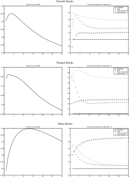
D. Variance Decompositions
That ignoring varying expected returns, or some component of time-varying expected returns, produces different valuations than the DDM is no surprise. What is more economically interesting is to investigate what is driving the time variation in the discount rates. We examine this by applying Corollary 2 to compute variance decompositions of the spot expected returns.
We first illustrate the volatility of the spot expected returns,var(µt(n)), at
each maturity in the left column of Figure 4. As the maturity increases, the volatility of the discount rates tends to zero. This is because asn→ ∞,µt(n)
approaches a constant because of stationarity, so var(µt(n))→0. At a 30-year
horizon, the µt(30) discount rate still has a volatility above 2.5% for growth
and neutral stocks, and above 7.0% for value stocks. While the volatility curve must eventually approach zero, it need not do so monotonically. In particular, for value stocks, there is a strong hump-shape, starting from around 4.7% at a 1-year horizon, increasing to near 8.0% at 13 years before starting to decline. The strong hump invar(µt(n)) for value stocks compared to growth and
neu-tral stocks is due to the much larger persistence of the value betas (0.84 com-pared to 0.68 (0.57) for growth (neutral) stocks in the VAR estimates of Table II). Note that the current beta is known in today’s conditional expected return. A shock to the beta only takes effect next period and the more persistent the beta, the larger the contribution to the variance of the discount rate.
Growth Stocks 0 5 10 15 20 25 30 0.02 0.025 0.03 0.035 0.04 0.045 0.05
Discount Curve Volatility
0 5 10 15 20 25 30 −0.4 −0.2 0 0.2 0.4 0.6 0.8 1
Variance Decomposition for BM Decile = 1
Cashflows Beta Risk−Free Rates Risk Premium Neutral Stocks 0 5 10 15 20 25 30 0.025 0.03 0.035 0.04 0.045 0.05
Discount Curve Volatility
0 5 10 15 20 25 30 0 0.1 0.2 0.3 0.4 0.5 0.6 0.7 0.8 0.9
Variance Decomposition for BM Decile = 6
Cashflows Beta Risk−Free Rates Risk Premium Value Stocks 0 5 10 15 20 25 30 0.045 0.05 0.055 0.06 0.065 0.07 0.075 0.08
Discount Curve Volatility
0 5 10 15 20 25 30 −0.2 0 0.2 0.4 0.6 0.8 1 1.2
Variance Decomposition for BM Decile = 10
Cashflows Beta Risk−Free Rates Risk Premium
Figure 4. Variance decomposition for the term structure of discount rates.The
left-hand column plotsvar(µt(n)), for eachnon thex-axis. The right-hand column attributes the
var(µt(n)) into proportions due to dividend growth, beta, the risk-free rate, and the risk premium.
![Figure 1. The spot discount curve µ t (n). The spot discount curve µ t (n) is used to discount an expected risky cashf low E t [D t +n ] of a security at time t + s back to time t](https://thumb-us.123doks.com/thumbv2/123dok_us/8734856.2366705/10.729.122.599.103.321/figure-discount-curve-discount-curve-discount-expected-security.webp)