Mathematical Discovery

(1)

Andrew M. Bruckner

University of California, Santa Barbara

Brian S. Thomson

Simon Fraser University

Judith B. Bruckner

ClassicalRealAnalysis.com

(2)

covery, especially to students who may not be particularly enthused about math-ematics as yet.

Cover Image: Photograph by xxxxxxxxxx.

Citation: Mathematical Discovery [Color Edition], Andrew M. Bruckner, Brian S.

Thomson, and Judith B. Bruckner, ClassicalRealAnalysis.com (2011), xv 253 pp. ISBN-13: 978-1463730574

ISBN-10: 1463730578

Date PDF file compiled: July 26, 2011

ISBN-13: 978-1463730574

ISBN-10: 1463730578

(3)

List of Figures

1 Andrew Wiles . . . -1

1.1 Checkerboard. . . 1

1.2 Greek mosaic made with square tiles. . . 1

1.3 Tiling a rectangle with squares . . . 2

1.4 Tiling a rectangle with four squares? . . . 3

1.5 Where is the smallest square? . . . 4

1.6 Where is the smallest square? (In a corner?) . . . 4

1.7 The smallest square has a larger neighbor. . . 5

1.8 The smallest square has two larger neighbors. . . 5

1.9 Possible Neighbor of the smallest square? (No.) . . . 6

1.10 Two possible neighbors of smallest square? (No.) . . . 6

1.11 Four possible neighbors of smallest square? (Maybe.) . . . 7

1.12 We try for a five square tiling. . . 8

1.13 a, b, c, d, and and s are the lengths of the sides of the “squares.” 8 1.14 A tiling with six squares? . . . 9

1.15 A tiling with seven squares? With nine squares? . . . 10

1.16 Will this nine square tiling work? . . . 10

1.17 A tiling with nine squares! . . . 11

1.18 Initial sketch for Arthur Stone’s eleven-square tiling. . . 12

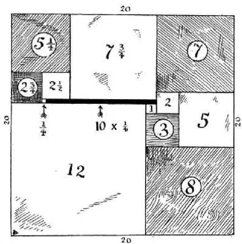
1.19 Can you reconstruct this figure from the numbers?. . . 13

1.20 Tiling a box with cubes.. . . 14

1.21 Equilateral triangle tiling. . . 15

1.22 Tutte and Stone. . . 16

1.23 Lady Isabel’s Casket (from a 1902 English book of puzzles). . . 17

1.24 The “solution” to Lady Isabel’s Casket. . . 18

1.25 More experiments with four squares. . . 20

1.26 We try for a five square tiling. . . 21

1.27 Lengths in terms of sides of 2 adjacent squares for Figure 1.15. . 22

1.28 Some square lengths labeled for Figure 1.15.. . . 22

1.29 Realization of Arthur Stone’s eleven-square tiling. . . 24

1.30 A 33 by 32 rectangle tiled with nine squares.. . . 25

1.31 A tower of cubes around K1. . . 26

1.32 S is the smallest triangle at the bottom of the tiling. . . . 27

(8)

1.33 T is the smallest triangle that touches S. . . . 28

2.1 What is the area of the region inside the polygon? . . . 29

2.2 A polygon on the grid. . . 31

2.3 Finding a line segment L that splits the polygon. . . . 32

2.4 A triangulation of the polygon in Figure 2.1. . . 33

2.5 Triangle with one vertex at the origin. . . 34

2.6 Decomposition for the triangle in Figure 2.5 . . . 35

2.7 The polygon P and its triangulation. . . 37

2.8 Too big and too small approximations . . . 37

2.9 Polygon P with 5 special points and their associated squares . . 39

2.10 A “skinny” triangle. . . 40

2.11 Some primitive triangles. . . 42

2.12 Polygons with 4 boundary points and 6 interior points . . . 43

2.13 Compute areas. . . 43

2.14 Split the rectangle into two triangles. . . 44

2.15 Adding together two polygonal regions. . . 46

2.16 A triangle with a horizontal base. . . 47

2.17 Triangles in general position. . . 48

2.18 Polygon P with border and interior points highlighted. . . . 49

2.19 Pick . . . 50

2.20 A primitive triangulation of a polygon. . . 52

2.21 A starting position for the game. . . 53

2.22 What is the area of the polygon with a hole? . . . 56

2.23 Rectangle P with one rectangular hole H. . . . 57

2.24 Random lattice. . . 60

2.25 Triangle on a random lattice. . . 61

2.26 Primitive triangulation of the triangle in Figure 2.25. . . 61

2.27 Sketch a primitive triangulation of the polygon. . . 62

2.28 Archimedes’s puzzle, called the Stomachion. . . 63

2.29 First quadrant unobstructed view from(0,0). . . 64

2.30 The six line segments that split the polygon. . . 66

2.31 Another triangulation of P. . . . 68

2.32 Obtuse-angled triangle T with a horizontal base.. . . 76

2.33 Acute-angled triangle T with a horizontal base. . . . 76

2.34 Triangles whose base is neither horizontal nor vertical. . . 77

2.35 What is the area inside P?. . . 78

2.36 Finding the line segment L. . . . 79

2.37 A final position in this game. . . 80

2.38 Polygon with two holes. . . 86

2.39 Several primitive triangulations of the polygon. . . 90

(9)

LIST OF FIGURES ix

3.1 A game of Nim. . . 95

3.2 Care for a game? . . . 96

3.3 A game with two markers at 4 and 9. . . 98

3.4 The ending position in a game with two markers. . . 99

3.5 A game with three markers at 4, 9, and 12. . . 100

3.6 The ending position in a game with three markers. . . 100

3.7 Position in the coin game.. . . 108

3.8 The same position in the coin game with binary bits. . . 109

3.9 A move in a 5_×3 game of binary bits. . . 110

3.10 Which positions are balanced? . . . 110

3.13 A game of Nim. . . 113

3.14 Coins set up for a game of Kayles. . . 115

3.15 The position(1,2,5,7,11)displayed in binary. . . 125

3.16 The move(1,2,5,7,11) (1,2,5,7,1)displayed in binary.. . . 126

3.17 Gaps in the 3–marker game with markers at 4, 9, and 13. . . . 127

3.18 Gaps in the 4–marker game with markers at 5, 10, 20, and 30. . 128

3.19 The three key gaps in the 6–marker game. . . 129

3.20 The 6–marker game with markers at 5, 7, 12, 15, 20, and 24. . 130

3.21 The 5–marker game with markers at 5, 10, 14, 20 and 22. . . . 131

3.22 An 8–marker game. . . 132

3.23 Last Year at Marienbad. . . . 133

3.24 A Reverse Nim game with 4 piles. . . 134

3.25 Two perspectives on Reverse Nim game with 4 piles. . . 134

3.26 Playing the associated 7–pile Nim game. . . 134

3.27 After the balancing move.. . . 135

3.28 An addition table for_⊕. . . 140

3.29 The game of 18 is identical to tic-tac-toe . . . 149

3.30 The card game is identical to tic-tac-toe . . . 149

3.31 Balancing numbers for 2–pile Nim.. . . 151

3.32 A position in the card game. . . 156

3.33 An odd position.. . . 159

3.34 How to change an odd position to an even position. . . 159

3.35 A position in the numbers game. . . 161

3.36 Playing the numbers game. . . 161

3.37 A position in the word game. . . 162

3.38 Balancing that same position in the word game. . . 163

3.39 A sequence of moves in a game of Kayles. . . 165

3.40 The same sequence of moves in a game of Kayles.. . . 166

3.41 Positions in the game(1,2,3). . . 167

(10)

4.1 Borromean rings (three interlinked circles). . . 181

4.2 Ballantine Ale . . . 182

4.3 Four circles. . . 182

4.4 Simple curves, closed curves or not? . . . 183

4.5 Equipment for making models. . . 184

4.6 Cole and Eva with model. . . 187

4.7 AB: First rotate the triangle T , then translate. . . . 205

4.8 BA: First translate the triangle T , then rotate. . . . 206

4.9 A “slips off” C. . . . 210

4.10 Projections of squares on the x-axis. . . . 211

4.11 This curve can be transformed into a circle. . . 213

4.12 Curve with “ear-like” twists. . . 213

4.13 Is C=AA−1? . . . 214

4.14 The three curves are linked in pairs. . . 215

4.15 A shoelace model of a 3–1 configuration. . . 216

4.16 Start with two separated circles for Problem 166. . . 216

4.17 Weave the curve through the circles. . . 217

4.18 Cut away the circle on the right. . . 218

4.19 Cut away the circle on the left. . . 218

4.20 AbBABb. . . 219

(11)

Preface

heu-ris-tic [adjective]

1. serving to indicate or point out; stimulating interest as a means of further-ing investigation.

2. encouraging a person to learn, discover, understand, or solve problems on his or her own, as by experimenting, evaluating possible answers or solutions, or by trial and error: a heuristic teaching method.

[Source: Dictionary.com]

Introduction

This book is an outgrowth of classes given at the University of California, Santa Barbara, mainly for students who had little mathematical background. Many of the students indicated they never understood what mathematics was all about (beyond what they learned in algebra and geometry). Was there any more math-ematics to be discovered or created? How could one actually discover or create new mathematics?

In order to give these students some sort of answers to such questions, we designed a course in which the students could actually participate in the discov-ery of mathematics. The class was not presented in the usual lecture fashion. And it did not deal with topics that the students had seen before. Ordinary al-gebra, geometry, and arithmetic played minor roles in most of the problems we addressed. Whatever algebra and geometry that did appear was relatively easy and straightforward.

Our objective was to give the students an appreciation of mathematics, rather than to provide tools they would need in some field that required mathemat-ics. In that sense, the course was like a course in music appreciation or art appreciation. Such courses don’t attempt to train students to become pianists, composers, or artists. Instead, they attempt to give the students a sense of the subject.

Why do so many intelligent people have so little sense of the field of ematics? A partial explanation involves the difficulty in communicating math-ematics to the general public. Without special training in astronomy, medicine, or other scientific areas, a person can still get a sense of what goes on in those areas just by reading newspapers. But this is much more difficult in

(12)

technical language that is difficult to express in ordinary English. Even profes-sional mathematicians often have difficulty communicating their work to other professional mathematicians who work in different areas.

This isn’t surprising when one realizes how many areas and sub areas there are in mathematics. Mathematical Reviews (MR) is a journal that provides short reviews of mathematical papers that appear in over 2000 journals from around the world. The subject classification used by MR has over 50 subject areas, each of which has several subareas. Each of these subareas has many sub-sub areas. A research mathematician might be an expert in several of the sub-sub areas, be conversant in several areas, and know very little about the other areas.

Objectives

Our objective is to impart some of the flavor of mathematics. We do this in several ways. First, by actively participating in the discovery process, a reader will get a sense of how mathematicians discover new mathematics.

A problem arises. Discovery often begins with some experimentation to help give a sense of what is involved in the problem. After a while one might have enough understanding of the problem to be able to make a plausible con-jecture, which one then tries to prove. The attempt to prove the conjecture can have several different outcomes. Sometimes the proof works. Other times it doesn’t work, but in trying to prove it one learns much more about the problem and identifies some stumbling blocks.

Sometimes these stumbling blocks seem insurmountable and one tries to prove they actually are insurmountable—the conjecture is false. That may cre-ate its own stumbling blocks. All the time one learns more and more about the problem. Finally one either proves the conjecture or disproves it. (Or simply gives up!).

We shall see all of this unfolding in the several chapters in the book. Our discovery process will be similar to that of a research mathematician’s, though our problems will be much less technical.

The first part of each chapter deals with a problem we wish to consider. We then go into the discovery mode and eventually obtain some answers. After this we turn to other aspects of mathematics related to the material of the chapter. What is the history of the problem? Who solved it? What are some related problems? How can other areas of mathematics be brought to bear on the prob-lem? Do computers have any role in solving the problems raised? What about conjectures that seemed to be true, but were eventually proven false? Or remain unsolved?

We have tried to find some balance between discovery and instruction. This is not always possible: it is impossible to resist the many occasions when some idea leads naturally to another wonderful idea. The reader will not discover the

(13)

connection, even with prodding, so we drop our heuristic approach and explain the new ideas. This is probably in the nature of things. When we look back on everything we have learned, certainly it is all a combination of stuff we figured out for ourselves and other stuff that we learned from others. It is the combination of the two that makes learning rewarding and productive. It is likely the stress on just the instruction part that explains the many people in this world who claim to dislike or fear mathematics.

Prerequisites

The main prerequisite for getting much from this book is curiosity and a will-ingness to attempt the problems we present. These problems usually set things up for the next stage in the discovery process. This is different from most text books, where the problems at the end of a section are intended to firm the read-ers’ knowledge of the material just presented.

Almost all problems have answers supplied at the end of the chapter. The word ANSWER following a problem indicates that an answer is supplied. For readers using a PDF file on a computer or laptop screen, that word is hyperlinked to the answer. Readers working on a paperback version will have to scan the end of the chapter to find the appropriate answer.

When the book is read in a self-study manner, rather than in a classroom setting with an instructor to set the pace, there may be a temptation to move ahead quickly, to get to the end of the process to learn the result. (Did the butler commit the crime?). We urge that one resist the temptation. The students who got the most out of the class were the ones who participated actively in the discovery process. This included working the problems as they arose. They said that understanding this process was of more value to them than learning the answer.

In order to understand the material in most of the chapters, one needs a bit of algebra (just enough to be able to manipulate some simple algebraic expres-sions, though such manipulations play only a very minor role), a bit of geometry, and a little arithmetic.

One topic that is not usually covered in a first course in algebra is math-ematical induction. This tool appears in several places. Readers not familiar with mathematical induction can reasonably work through a chapter that has an induction argument until that argument is needed. At that point, one can consult the Appendix where induction is discussed and induction proofs are given that are relevant to various problems we discuss. Induction does not take part in the discovery process—it is used only to verify that certain statements are true.

(14)

Professional mathematicians must be rigorous in their work. This involves giv-ing careful definitions, even of apparently familiar objects. This often involves a great deal of “technical machinery.” A mathematician needs to know such things as exactly what a “curve” is, what it means to “go around a curve so that the inside is to the left,” how to mathematically describe the number of “holes” in a pretzel and the meaning of area.

It should be understood, however, that this is not the situation when a math-ematician first starts thinking of a problem and working out a solution. Things are rather vague and intuitive in the early stages. The polish and rigor appear in full force only in the final drafts.

Since this book is not intended for mathematicians, who would require for-mal definitions and proofs, we can relax these requirements considerably. Ev-erything we say in an informal way can be said in a mathematically rigorous way, but that is not our purpose. Our purpose is to provide some of the flavor of mathematics and introduce the reader to topics that some students were sur-prised to find involved mathematics. Thus we can take for granted that readers intuitively understand concepts such as curves, inside, left, holes, and area. We will occasionally describe a concept with which the reader may not be familiar, but our overall style is primarily a leisurely, informal one.

Acknowledgements

The authors are grateful to many who have contributed in one way or another to the creation of this book. In particular, the many students who participated in the classes contributed greatly. They pointed out difficulties, found interesting solutions to problems that were different from our solutions, provided reason-able approaches to problems that sometimes worked and sometimes didn’t, but were often creative whether or not they worked.

We also want to acknowledge Professor Steve Agronsky who used prelim-inary versions of this book in his classes at Cal. Poly. University in San Luis Obispo, California. He made a number of useful suggestions based on his teach-ings .

Most of the figures were prepared by us using Mathematica.TM A number of the figures were found on the internet and, naturally enough, it has proved to be difficult to give proper attribution. Any person who is the original author of such figures is invited to write to us with instructions as to whom to give proper credit. We are thankful for those who have released such figures to the public domain and will be equally thankful to those who wish credit.

We are always grateful for comments and will attempt to incorporate them into future printings (or future editions) with explicit acknowledgement of the sources. Please write to the authors at thomson asfu.ca.

(15)

To the Instructor

One might notice that, on occasion, one or more problems follow after only a short discussion. This occurs when we believe this short discussion already presents an opportunity for the reader to get a sense of how we might continue. When we taught the class, we often found it convenient to make a small amount of progress on each of two chapters in one class session. How this worked in practice varied with what happened in class discussion. Sometimes the material we list as problems actually became part of the class discussion, rather than as problems to be discussed at the next class session. It worked best to be flexible and see where the discussion took us in determining whether we should solve some of the problems in lecture form, or leave them as problems to be discussed in the next class meeting.

In a typical one-quarter term we would have covered four chapters in a leisurely fashion, at least through the discovery of the solution to the main prob-lems of the chapter. We also were able to cover some of the material at the end of the chapters. Available time, class interests, and level of difficulty relative to the students’ backgrounds determined what we covered.

We provide answers to most of the problems, in particular to those that point the way to further progress. We leave a few unanswered. Some of these we used as quizzes or homework to be collected.

(16)

(17)

“Perhaps I can best describe my experience of doing mathemat-ics in terms of a journey through a dark unexplored mansion. You enter the first room of the mansion and it’s completely dark. You stumble around bumping into the furniture, but gradually you learn where each piece of furniture is. Finally, after six months or so, you find the light switch, you turn it on, and suddenly it’s all illu-minated. You can see exactly where you were. Then you move into the next room and spend another six months in the dark. So each of these breakthroughs, while sometimes they’re momentary, some-times over a period of a day or two, they are the culmination of— and couldn’t exist without—the many months of stumbling around in the dark that preceed them.”

“I used to come up to my study, and start trying to find patterns. I tried doing calculations which explain some little piece of math-ematics. I tried to fit it in with some previous broad conceptual understanding of some part of mathematics that would clarify the particular problem I was thinking about. Sometimes that would in-volve going and looking it up in a book to see how it’s done there. Sometimes it was a question of modifying things a bit, doing a little extra calculation. And sometimes I realized that nothing that had ever been done before was any use at all. Then I just had to find something completely new; it’s a mystery where that comes from. I carried this problem around in my head basically the whole time. I would wake up with it first thing in the morning, I would be think-ing about it all day, and I would be thinkthink-ing about it when I went to sleep. Without distraction, I would have the same thing going round and round in my mind. The only way I could relax was when I was with my children. Young children simply aren’t interested in Fermat. They just want to hear a story and they’re not going to let you do anything else.”

Figure 1: Andrew Wiles

— Andrew Wiles

In an interview for PBS TV program Nova on the oc-casion of his solving Fermat’s Last Theorem.

(18)

(19)

Chapter 1 Tilings

It is easy to imagine a rectangle tiled with squares. The familiar checkerboard in Figure1.1is a tiling of a square by sixty-four smaller squares.

Figure 1.1: Checkerboard.

A little more artistically, the tiling in Figure1.2shows a rectangle that has been tiled into a number of smaller squares arranged in an attractive design.

Figure 1.2: Greek mosaic made with square tiles.

In both these cases all the squares are of equal size. This is familiar in the pattern we see for checkerboards or for many ceramic tilings of kitchen floors. But what if the squares are not all of the same size?

Figure1.3 has tiles of unequal size but many of them are of the same size. What if we insist that no two of the squares can be of the same size. A few moments of thought shows that this problem is much, much harder.

How does one begin to discover such constructions? Perhaps after trying to find one you will give up in frustration and suspect that no such tiling can exist.

(20)

Figure 1.3: Tiling a rectangle with squares

We don’t recognize this as a problem that we can attack by any of the stan-dard methods of arithmetic, algebra or geometry. This is a situation that often arises in creative mathematics. We are faced with a problem but are at a loss about what tools to bring to bear on the problem. What to do? Faced with this type of problem, the creative mathematician would probably begin by trying to get a feel for the problem by experimenting with a few examples.

1.1 Squaring the rectangle

The problem of tiling a rectangle with unequal sized squares has been described by some as the problem of squaring the rectangle. We do not know in advance on starting to look at such a problem whether there is a solution, and if there is a solution how we should go about finding one.

Perhaps we should begin by seeing whether we can put together a few squares (no two of the same size) in such a way that they combine to form a rectangle. (At this stage, it’s almost like working a jig-saw puzzle.)

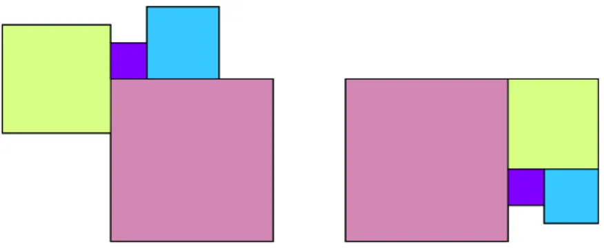
Let’s start with a small number of squares. A moment’s reflection reveals that it is impossible to achieve our desired result with only two or three squares. With four squares, there are quite a few ways in which the squares can be com-bined. Figure1.4shows two possibilities that you might have tried.

Problem 1 Experiment with four, five, and six squares. That is, try to combine

the squares in such a way that the resulting figure is a rectangle. Remember

(21)

1.1. SQUARING THE RECTANGLE 3

Figure 1.4: Tiling a rectangle with four squares?

1.1.1 Continue experimenting

Did you find a tiling of a rectangle by four, five, or six squares, all of different sizes? If so, check again. Are two of the squares the same size? You do not need a ruler to check this. Simply put in the numbers which you think repre-sent the lengths of the sides of the squares and see if everything adds up right. For example, we might think that the configurations in Figure1.4 are possible after all. Maybe our drawing program does not quite get the job done, but the configuration there is possible with the right choice of dimensions.

The chances are that you did not arrive at a solution to the problem. It must also have become clear that as the number of squares we use in our experi-menting increases, the number of essentially different configurations we can put together increases rapidly. Even with six squares, the number of configura-tions we can try is very large—and it gets much worse if we tried to use seven or eight tiles.

How should we proceed? Our experimenting has not brought us a solution to the problem. But that does not mean it was a waste of time. We may have learned something.

1.1.2 Focus on the smallest square

For example, we may have noticed that many of our attempts led to a certain difficulty. Perhaps we can find a way to overcome this difficulty. Or, perhaps it is impossible to overcome, thereby making the problem one with no solution. What is this difficulty? Consider again, for a moment, the configurations that you tried out while working on Problem1. For each of these look to see where you placed the smallest square.

(22)

Figure 1.5: Where is the smallest square?

five or six tiles. If we were able to complete these attempts by adding more tiles, these small spaces could accommodate only tiles which are small enough to fit into the space. And this would create even smaller spaces, to be filled with even smaller tiles. We can certainly continue to add smaller and smaller tiles, but at some point the process must stop if we are to arrive at a solution to our problem. At this point it may look hopeless. Perhaps we can use what we have learned to prove that there is no solution to the problem that uses only four, five or six squares.

1.1.3 Where is the smallest square

Let us focus on the difficulty we encountered. If there is a solution, there must be a smallest square S. And that smallest square S must fit into the picture somewhere. Where? Maybe we can show that there is no place for it to fit.

This is what our experimenting showed — whenever the smallest square was in one of our trials, there was a space neighboring it which could accommodate only still smaller squares. (This might not have been true of all our trials, but it probably was true of most of those trials that offered any hope of success.) Where could the smallest square fit? Could it be in a corner as in Figure1.6?

S

(23)

Is the smallest square in a corner? A moment’s reflection shows it can’t be. Since S is the smallest square, its neighbors must be larger as in Figure1.7.

S

Figure 1.7: The smallest square has a larger neighbor.

But that creates exactly the kind of space we’ve been talking about. Only squares smaller than S could fit into that space.

Is the smallest square on a side? Similarly, we see that S cannot be on one of the sides of the rectangle as Figure1.8illustrates.

S

Figure 1.8: The smallest square has two larger neighbors.

It’s two neighbors on that side must be larger than S; once again a small space is created. So, if there is a solution to the problem at all, the smallest square must lie somewhere inside the rectangle, i.e., its sides cannot touch the border of the rectangle.

Problem 2 Do you think it is possible to find a tiling using exactly four squares

of unequal size?

Problem 3 Do you think it is possible to find a tiling using exactly five or six

squares of unequal size?

1.1.4 What are the neighbors of the smallest square?

(24)

Let’s analyze a bit more. Suppose there is a solution and S is the smallest square. We know S must be inside the rectangle. What possibilities are there for the relationship between S and its neighbors?

S

Figure 1.9: Possible Neighbor of the smallest square? (No.)

A possible case? A neighbor of S might extend beyond S on both sides as Figure1.9illustrates. This, we see is not possible because two other neighbors (the ones below and above S in the diagram) would then create a small space.

Another possible case? The smallest square S may have a side bordering on two neighbors as Figure1.10illustrates. This is impossible for the same reason.

S

Figure 1.10: Two possible neighbors of smallest square? (No.)

The only possible case! Each neighbor of the smallest square S has a side which fully contains one side of S, but extends on one side of S only. Figure1.11

illustrates this. Is this possible? At least no small space has been created. This is the only case we cannot rule out immediately.

(25)

S

Figure 1.11: Four possible neighbors of smallest square? (Maybe.)

We have not determined that a solution exists. But we have learned something about what a solution must look like (if there is a solution at all).

This leaves us with two options: we could continue to try to show there is no solution. How might we try? Perhaps we can still show that there is no place to put S. Or maybe the second smallest square creates a problem. Our alternative is to switch gears again and try to show there is a solution. If we take this positive option, we are far better off than we were at the beginning. We need try only such constructions which have the smallest square surrounded by its neighbors in a windmill fashion. Let’s try that for awhile and see what it leads to.

Problem 4 Experiment with four, five, and six squares trying to combine the

squares in such a way that the resulting figure is a rectangle. (Same as Prob-lem1, but use newly learned information.)

Answer

1.1.5 Is there a five square tiling?

It is clear that we need not try to find a solution with four squares. One thing we’ve already learned is that a solution (if one exists) requires at least five squares, namely S and its four neighbors. Let’s try a solution with five squares. Such a solution must involve S surrounded by its neighbors in a windmill fash-ion. Figure1.12 illustrates an attempt at this. In the figure A, B, C and D are squares surrounding a central square S.

Careful measurements of the sides of the squares in this configuration will reveal that they are not exactly squares. (And we want them exactly squares.) But that may mean no more than that we weren’t careful with our drawing. And, after all, no one can draw a perfect square! One would hardly discard the idea of a circle just because no one can draw a perfect circle.

(26)

S

A

B

C

D

Figure 1.12: We try for a five square tiling.

numbers representing the sides of the squares so that all the requirements of our problem are satisfied.

An algebraic method To check that a proposed solution is correct or to prove that a proposed solution is impossible, we can use some simple algebra. Sup-pose the diagram represented a solution. Denote the length of the side of S by s and the length of the side of A by the letter a. The labeling is shown in Figure1.13.

mv Tile

s

a

b

c

d

Figure 1.13: a, b, c, d, and and s are the lengths of the sides of the “squares.”

Then, B has side length s+a (why?) so C has side length

s+ (s+a) =2s+a

and D has side length

s+ (2s+a) =3s+a.

(27)

The only other possible five-square configuration using our windmill idea would look similar to this and would check out negatively too. To this point, then, we have proved that it is impossible to solve our problem with five or fewer squares.

1.1.6 Is there a six, seven, or nine square tiling?

In the problems below determine whether the suggested configurations can work. Don’t go by the accuracy of the drawing. Just because some of the tiles don’t look like squares doesn’t mean that one can’t distort the picture some, keeping each tile in its same relationship to its neighbors, and making all the tiles squares. In some cases you may need to use the algebraic technique of this section.

Problem 5 Does this configuration in Figure1.14of six “squares” work?

Figure 1.14: A tiling with six squares?

Answer

Problem 6 Does the configuration of seven “squares” in Figure1.15work? Answer

Problem 7 Does the configuration of nine “squares” in Figure1.15work? Answer

Problem 8 Experiment some more. Construct diagrams like those in

Prob-lem5, Problem6and Problem7.

(28)

Figure 1.15: A tiling with seven squares? With nine squares?

1.2 A solution?

While working on Problem8you may have succeeded in arriving at a diagram such as the one that appears in Figure1.16. We don’t have to sketch it accu-rately; the figure suggests another possible configuration that might look like this. As usual, for our method, the smallest square is labeled as s and its neigh-bor as a. The rest of the side lengths would then be determined as the figure shows.

3 a

₊

2 s

2 a

₊

s

a

₊

s

_a

4 a

₊

4 s

s

a

-

s

4 a

5 a

_-

s

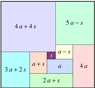
Figure 1.16: Will this nine square tiling work?

Can this configuration be made into a solution? That is, can values of s and a be found so that all the rectangles are squares? Since the right and left sides of the rectangle must have the same length, we calculate

(29)

1.2. A SOLUTION? 11

or

7s=2a.

If, for example. we take a=7 and s=2 we would have 7s=2a and we would arrive at the following diagram in Figure1.17, the tiny square having side 2.

25

16

9 ₇

36

2

5

28

33 Elements: 2, 5, 7, 9, 16, 25, 28, 33, 36

Figure 1.17: A tiling with nine squares!

Thus, we see there is a solution to the nine square problem after all. And, to be sure, the diagram that we and you used for this solution would not have had tiles that looked like squares (unlike the final neat graphics here) but the algebra verified that we can create a tiling meeting all our conditions.

Problem 9 Here is the algebraic method of this section as described by William

T. Tutte (1917–2002), one of the founders of this theory:

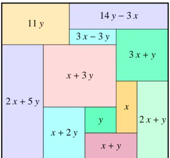
“The construction of perfect rectangles proved to be quite easy. The method used was as follows. First we sketch a rectangle cut up into rectangles, as in [Figure1.18]. We then think of the diagram a bad drawing of a squared rectan-gle, the small rectangles being really squares, and we work out by elementary algebra what the relative sizes of the squares must be on this assumption. Thus in [Figure1.18] we have denoted the sides of two adjacent small squares by x and

y and then that the side of the square next on the left is x+2y, and so on. Pro-ceeding in this way we get the formulae . . . for the sides of the 11 small squares. These formulae make the squares fit together exactly . . . . This gives the perfect rectangle . . . the one first found by [Arthur] Stone.” ——W. T. Tutte [12].

Carry out all the arithmetic needed to construct Figure 1.18, the initial sketch for Stone’s tiling. Then do the necessary algebra to find the sides of

(30)

2 x

₊

5 y

x

₊

2 y

y

x

₊

y

2 x

₊

y

x

₊

3 y

3 x

₊

y

11 y

14 y

-

3 x

_-

3 y

Figure 1.18: Initial sketch for Arthur Stone’s eleven-square tiling.

1.2.1 Bouwkamp codes

Our solution of the rectangle in Figure1.17tiled with nine squares is something we might want to keep a record of and communicate to others. If we send someone a picture they can easily check that we have it all right and can see exactly what our solution is. Suppose we communicate only the size of the smaller squares:

2, 5, 7, 9, 16, 25, 28, 33, 36.

A little more helpful would be to indicate also the size of the large rectangle, in this case

61_×69.

In theory that should be enough for someone who likes fiendish puzzles, but these numbers alone don’t tell the story in any adequate way. The picture does, but that is an inefficient way to communicate our ideas.

The Dutch mathematician Christoffel Jacob Bouwkamp (1915–2003) de-vised a simple code that is much used nowadays. Problem 10asks you to de-vise your own code, but the answer (found at the end of the chapter) gives the Bouwkamp code and a brief description of how it works.

(31)

1.2. A SOLUTION? 13

33 37 42

29 25 ₁₆

9 7

18 24

50

35 27

15 17 11

19 8

6

4

2

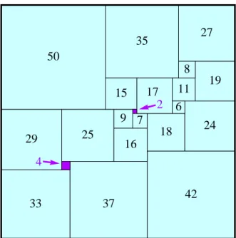
Figure 1.19: Can you reconstruct this figure from the numbers?

Answer

Problem 11 Give the Bouwkamp code for Figure1.17. Answer

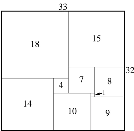
Problem 12 Here are the Bouwkamp codes for the only ninth order squared

rectangles. Construct the one that is not in the text already.

Order 9, 33 by 32: (18,15)(7,8)(14,4)(10,1)(9) Order 9, 69 by 61: (36,33)(5,28)(25,9,2)(7)(16)

Answer

1.2.2 Summary

Let us reflect on where we have been so far in this chapter. We started with an interesting (but puzzling) geometric problem. It was unlike the usual high-school geometry problems in that none of the usual techniques of geometry could be brought to bear on the problem.

At first, the problem wasn’t one for which we had any ideas at all for a solution. So we played around with it in the hopes of learning something. What we learned by experimenting enough was that there was a difficulty caused by the small space adjoining the smallest square in most of our attempts. Maybe that was the key to the problem. Perhaps there was no solution, and perhaps we could prove that by showing there’s no place for the smallest square.

(32)

We returned to the drawing boards, armed with our new information. Eventu-ally we were able to use a bit of algebra together with what we learned to arrive at a solution.

So we’ve solved our problem. Now what? A creative mathematician might ask a lot of questions suggested by this problem. Which rectangles can one tile with squares? Are there any squares that can be tiled with unequal squares? What other tilings are possible or impossible?

For additional examples of tilings, see Stein [9]. In that reference one can find a leisurely development of a number of questions related to tiling. In partic-ular, a surprising way in which tiling and electrical theory are related is devel-oped there and leads to the theorem that if a rectangle can be tiled with squares in any manner whatsoever, then it can also be tiled by squares all of the same size.

We will continue with some related material for those readers who want to purse these ideas further. For mathematicians no problem ever stops cleanly: there are always some more questions to address, more ideas that our investiga-tion suggests.

1.3 Tiling by cubes

What about tilings with other types of figures? One can ask analogous questions in higher dimensions. Is it possible to fill a rectangular box with cubes no two of which are the same size (as suggested in Figure 1.20)? This is the three dimensional version of the problem we just solved. At first glance it appears to be much more difficult. But, perhaps some of the insights we picked up from the two-dimensional case can be of use to us in this three dimensional version.

Figure 1.20: Tiling a box with cubes.

Problem 13 Determine whether or not it is possible to fill a three-dimensional

(33)

1.4. TILINGS BY EQUILATERAL TRIANGLES 15

1.4 Tilings by equilateral triangles

Figure1.21shows a tiling of an equilateral triangle with other equilateral trian-gles, but notice that there are several duplications of same sized triangles in the figure.

Figure 1.21: Equilateral triangle tiling.

Similar ideas to those developed so far in the chapter are useful in showing that it is impossible to tile an equilateral triangle with other equilateral triangles no two of which are the same size. Problem14asks you to do this.

1.4.1 (Tutte, 1948) If an equilateral triangle is tiled with other equilateral

trian-gles then there must be two of the smaller triantrian-gles of the same size.

This was first proved by W. T. Tutte in 1948 (see item [11] in our bibliogra-phy). An accessible account of this problem appears as the chapter

W. T. Tutte, Dissections into equilateral triangles (pp. 127–139)

in the book by David Klarner that is reference [16] in our bibliography. A 1981 article by Edwin Buchman in the American Math. Monthly (see [15]) shows, using Tutte’s methods, that there is no convex figure at all that could be tiled by equilateral triangles unless at least two of those triangles are the same size.

For further discussion of these topics see the book of Sherman Stein [9] that appears in our bibliography.

Problem 14 Show that it is not possible to tile an equilateral triangle with

(34)

1.5 Supplementary material

We conclude our chapter with some supplementary material that the reader may find of interest in connection with the problem of squaring the rectangle.

1.5.1 Squaring the square

We have succeeded in tiling some rectangles with unequal squares but none of our rectangles was a square itself. Is it possible to assemble some collection of unequal squares into a square?

The description of the problem as squaring the square originates with one of the four Cambridge University students Tutte, Brooks, Smith, and Stone who attacked the problem in 1935. It was intended humorously since it seems to allude to the famous problem of squaring the circle which means something totally different and was well-known to be impossible.

Tutte in his autobiographical memoir1 describes Arthur H. Stone (1916-2000) as the one of the four who proposed the problem. He had found an old puzzle in a book of Victorian puzzles written by Henry Dudeney, an English puzzler and writer of recreational mathematics.

Figure 1.22: Tutte and Stone.

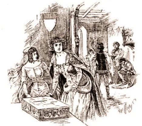
See Figure1.23 for Dudeney’s statement of his problem. The “solution” of the problem in the book is given by Dudeney in Figure1.24 where the inlaid strip of gold is the black rectangle in the middle. The problem is called Lady Isabel’s Casket. (In Victorian England a casket was not necessarily just for containing corpses, but could be “a small box or chest, often fine and beautiful, used to hold jewels, letters or other valuables” [as defined in the World Book Dictionary].)

(35)

1.5. SUPPLEMENTARY MATERIAL 17

(36)

Figure 1.24: The “solution” to Lady Isabel’s Casket.

Stone realized that the problem was tougher than Dudeney had thought, for, if this figure were indeed the unique solution of the problem, that could only mean that none of the squares in the figure could be divided into smaller un-equal squares. They learned that the great Russian mathematician Nikolai Niko-laievich Lusin (1883–1950) had conjectured that no square could be squared. Thus the four of them decided that they could make their reputation by solving this Lusin Conjecture: no square can be subdivided into a collection of squares no two of the same size.

In fact they not only succeeded in squaring the square but in finding deep connections to the problem with graph theory and electrical networks.

The smallest squared-square Did you notice that Figure 1.19is a squared-square? Problem10asked for the Bouwkamp code for this tiling by twenty-one unequal squares. This is the lowest order example of squaring the square.

(37)

1.5. SUPPLEMENTARY MATERIAL 19

This gives a tiling of S.

A final word. The problem that began this chapter was to determine whether it is ever possible to tile a rectangle with squares of unequal sizes. We answered this question in the affirmative. The question remains which rectangles can be tiled in this manner. The answer to this question is given following the answer to Problem19.

1.5.2 Additional problems

For those readers who did not get enough problems to work on here are some more. We also have added some more Bouwkamp codes problems as they ap-pear to be popular entertainments (much like Suduko problems). Note that with these codes one can design jig-saw puzzles consisting of unequal squares which must be assembled to form a large rectangle. The Bouwkamp codes themselves then are quick descriptions of how to assemble the pieces to solve the puzzle.

Problem 15 Here are the Bouwkamp codes for all of the tenth order squared

rectangles. Sketch the tiling figures for as many of these as you find entertaining.

Order 10, 105 by 104: (60,45)(19,26)(44,16)(12,7)(33)(28) Order 10, 111 by 98: (57,54)(3,7,44)(41,15,4)(11)(26) Order 10, 115 by 94: (60,55)(16,39)(34,15,11)(4,23)(19) Order 10, 130 by 79: (45,44,41)(3,38)(12,35)(34,11)(23) Order 10, 57 by 55: (30,27)(3,11,13)(25,8)(17,2)(15) Order 10, 65 by 47: (25,17,23)(11,6)(5,24)(22,3)(19)

Problem 16 Here are the Bouwkamp codes for all of the eleventh order squared

rectangles. If this still amuses you, sketch some more figures.

(38)

Order 11, 209 by 177: (96,56,57)(55,1)(58)(81,15)(66,4)(62) Order 11, 97 by 96: (56,41)(17,24)(40,14,2)(12,7)(31)(26) Order 11, 98 by 86: (51,47)(8,39)(35,11,5)(1,7)(6)(24) Order 11, 98 by 95: (50,48)(7,19,22)(45,5)(12)(28,3)(25)

Problem 17 If a rectangle is tiled by squares, all of different sizes, the second

smallest square cannot touch the border of the rectangle. Prove this

statement.-Problem 18 Suppose we are given a rectangle of dimensions a_×b. Can this

rectangle be subdivided into equal sized squares? Answer

Problem 19 Suppose we are given a rectangle of dimensions a_×b. Under what circumstances can you be sure that this rectangle cannot be subdivided into a

finite number of (not necessarily equal) squares? Answer

1.6 Answers to problems

Problem

1, page 2

Figure1.25 shows some possibilities with four unequal squares that you might have tried. These two are unsuccessful.

Figure 1.25: More experiments with four squares.

Problem

4, page 7

(39)

1.6. ANSWERS TO PROBLEMS 21

get the dimensions right? Our drawing program won’t produce accurate squares but the layout looks promising.

Before reading on in the text, try to see if you can find dimensions that would make this configuration work. Label the side lengths of the squares and see if there are numbers that work. If you can show that there cannot be such numbers then you will have succeeded in showing that this particular arrangement does not work.

S

A

B

C

D

Figure 1.26: We try for a five square tiling.

Problem

5, page 9

In the figure of Problem5, we see that two of the tiles have a common side. If they are to be squares, they must be the same size, violating a condition of our problem. Thus we do not need to do the algebra. A tiling that looks like this does not solve our primary problem: find a tiling with all squares of different sizes.

Problem

6, page 9

In the figure for Problem 6, we see a plausible configuration. None of the squares (if indeed they could be squares) is the same size as any of the oth-ers. We need to find exact numbers that would make this work.

(40)

s

a

₊

2 s

a

2 a

_-

s

a

_-

s

3 a

_-

2 s

a

₊

s

Figure 1.27: Lengths in terms of sides of 2 adjacent squares for Figure1.15.

Since the top and bottom of a rectangle are of equal length,

3s+2a=5a₋3s

so that 2s=a. Thus two of the rectangles would have to have sides equal to 3s. Again this violates our primary objective: find a tiling with all squares of different sizes. Did you notice that other requirements are violated?

Problem

7, page 9

Again we see no immediate objection to this configuration: it might work. Let’s do our algebraic computations. There are several ways to do this. Here’s one in Figure1.28. that gives us the sizes of some of the squares. We now compute that the darkest square in the figure has side

(a₋3s)₋a₋s=₋4s.

This is again impossible, now because we have produced a negative number for the length of a side.

a

_-

2 s

s

a

_-

3 s

a

_-

s

(41)

Remark Note that our arguments never involved a statement such as “this tile is much too thin to be a square.” Even if we had been correct with such a statement, this would not rule out a similar configuration in which all the tiles were squares.

Such a configuration could possibly have been achieved by proper vertical and horizontal stretchings of the entire configuration. But our arguments in all three of the problems in this section showed that something was inherently wrong with the ways some of the tiles related to their neighbors. One couldn’t stretch the configurations and render all the tiles squares of different sizes.

Problem

8, page 9

0.K. We are now ready to take another crack at finding a solution. We have a simple and easy to apply algebraic method for checking our proposed solution. We know in advance where to place the smallest square.

If our attempts fail, perhaps we can discover some unresolvable difficulty inherent in the problem. If we can prove that there is such an inherent unre-solvable difficulty, then we will have proved the problem has no solution. Many problems posed in mathematics have no solution and we might be equally proud of showing that the problem is impossible as finding an answer.

But first, experiment some more.

(42)

Problem

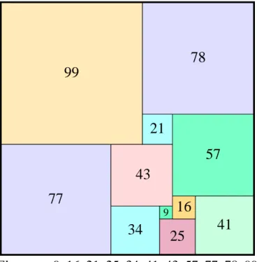
9, page 11

77

34

9

25

41

16

43

57

99

78

21

Elements: 9, 16, 21, 25, 34, 41, 43, 57, 77, 78, 99

Figure 1.29: Realization of Arthur Stone’s eleven-square tiling.

The dimensions of Stone’s tiling are shown in Figure1.29. Just do the elemen-tary algebra using the same method that we used and you should be able to discover all of the dimensions. You may wish to compare the length of the side of the rectangle in the upper right hand corner with the lengths of the sides of the two rectangles below it to obtain 16y=9x.

Problem

10, page 12

A reasonable start at communicating the configuration in Figure1.19 is to start at the upper left corner and report the adjacent squares at the top from left to right:

50, 35, 27.

(43)

In the Bouwkamp code, brackets are used to group adjacent squares with flush tops, and then the groups are sequentially placed in the highest (and left-most) possible slots. For this example of the 21-square illustrated in the problem the code is

[50,35,27], [8,19], [15,17,11], [6,24], [29,25,9,2], [7,18], [16], [42], [4,37], [33].

Problem

11, page 13

[36,33], [5,28], [25,9,2], [7], [16].

Problem

12, page 13

14

18

15

4

10 ₉

7

1

8

32

33

Figure 1.30: A 33 by 32 rectangle tiled with nine squares.

In Figure1.30is a picture that corresponds to the Bouwkamp code

(44)

Problem

13, page 14

It is a bit more difficult to experiment with the three-dimensional setting than it was with the two-dimensional setting. The remark before the problem suggests that “some of the insights we picked up from the two dimensional case can be of use to us in this three dimensional version.” The key in two dimensions was the use of the smallest square argument. Try this:

Use the smallest cube argument!

Don’t read the rest of the answer without trying again. You may wish to glance at Figure1.31.

Our proof is an indirect one. We assume that there is such a construction and find that there is a contradiction.

Suppose a rectangular box were filled with cubes no two of which were of the same size. Consider only those cubes which lie on the bottom of the box. The bottom faces of these cubes tile the floor of the box by squares, no two of the same size. The smallest of these tiles must be surrounded by four other tiles in a windmill fashion. Let K1be the smallest of the cubes lying on the floor of

the box. From what we just said, we see that K1 is surrounded by four larger

cubes which form a tower around K1as suggested in Figure1.31.

Figure 1.31: A tower of cubes around K1.

Now consider those cubes whose bottoms lie on the top face of K1. Their

(45)

these K2is surrounded by four larger cubes which form a tower around it.

Continuing in this manner we see there can be no end to this process. No matter how many of these cubes K1, K2, K3, . . . we have obtained, there must

still be smaller ones lying on top of the smallest obtained to that point. Thus, we have proved this:

1.6.1 (No cubing the box) It is impossible to fill a rectangular box with cubes,

all of different sizes.

Our techniques in the tiling problem of studying the location of the small-est square was useful to us in two ways: firstly, it gave us information about the structure of tilings of rectangles by squares of different sizes—the small-est square must be surrounded in a certain way by its neighbors; secondly. It suggested an approach to solving the analogous problem in three dimensional space.

Problem

14, page 15

The smallest cube argument that succeeded for Problem 13 suggests that a smallest triangle argument can be developed for this problem, and indeed very similar ideas will work here.

Our proof is again an indirect one. We assume that there is such a construc-tion and find that there is a contradicconstruc-tion.

Assume that we have a tiling by smaller equilateral triangles, all of different sizes. Start by looking for the smallest triangle S that touches the bottom of the triangle. Argue that it must look like Figure1.32.

S

Figure 1.32: S is the smallest triangle at the bottom of the tiling.

Then look for the smallest triangle T that touches the top of the triangle S. Argue that it must look like Figure1.33. This argument keeps going indefinitely and so we shall soon run out of triangles, just as in our solution to Problem13

(46)

S

T

Figure 1.33: T is the smallest triangle that touches S.

Problem

18, page 20

To begin the problem check that, when a and b are integers then the rectangle can be easily subdivided into ab equal sized squares, all of side length 1.

Suppose a or b is not an integer and a/b can be expressed as a fraction m/n, where m and n are positive integers. Then a=cm and b=cn for some number c. Thus take small squares of side length c and there are certainly mn such squares fitting inside the rectangle.

If a/b is not a fraction (i.e., it is an irrational number) then there would be no choice of side length c for the small squares to work out. In modern language two real numbers a and b are commensurable if a/b is a rational number (i.e., a fraction). Thus the answer to the problem is that we must require a and b to be commensurable.

Problem

19, page 20

We just saw in Problem18that a rectangle R cannot be tiled with equal squares unless the sides of the rectangle are commensurable. It is also true for any tiling by a collection of squares that this same condition must be met. A proof that a rectangle can be so tiled if and only if a and b are commensurable is given in

R. L. Brooks, C. A. B. Smith, A. H. Stone and W.T. Tutte, The dissection of rectangles into squares, Duke Math. J. (1940) 7 (1): 312–340.

Probably the first proof of the theorem that a rectangle can be squared if and only if its sides are commensurable is by Max Dehn,

Max Dehn, Über Zerlegung von Rechtecken in Rechtecke, Mathe-matische Annalen, Volume 57, September 1903.

(47)

Chapter 2 Pick’s Rule

Look at the polygon in Figure2.1. How long do you think it would take you to calculate the area? One of us got it in 41 seconds. No computers, no fancy cal-culations, no advanced math, just truly simple arithmetic. How is this possible? The projects in this chapter have as their centerpiece work published in 1899 by Georg A. Pick (1859–1942). His theorem supplies a remarkable and simple solution to a problem in areas. Set up a square grid with the dots equally spaced one inch apart and draw a polygon by connecting some of the dots with straight lines. What is the area of the region inside the polygon?

P

Figure 2.1: What is the area of the region inside the polygon?

You will likely imagine counting up the number of one-inch squares inside and then making some estimate for the partial squares near the outside. Pick’s Rule says that the area can be computed exactly and quickly: look at the dots!

As is always the case in this book, it is the discovery that is our main goal. Many mathematics students will learn this theorem in the traditional way: the theorem is presented, a few computations are checked, and the short inductive proof is presented in class. We take our time to try to find out how Pick’s formula might have been discovered, why it works, and how to come up with a method of proof.

(48)

2.1 Polygons

In Figure 2.1 we have constructed a square grid and placed a polygon on that grid in such a way that each vertex is a grid point. The main problem we address in this chapter is that of determining the area inside such a polygon. We need to clarify our language a bit, although the reader will certainly have a good intuitive idea already as to what all this means.

Familiar objects such as triangles, rectangles, and quadrilaterals are exam-ples. Since we work always on a square grid the line segments that form the edges of these objects must join two dots in the grid.

2.1.1 On the grid

We can use graph paper or even just a crude sketch to visualize the grid. For-mally a mathematician would prefer to call the grid a lattice and insist that it can be described by points in the plane with integer coordinates1.

But we shall simply call it the grid. It will often be useful, however, to describe points that are on the grid by specifying the coordinates.

Problem 20 A point (m,n) on the grid is said to be visible from the origin

(0,0)if the line segment joining(m,n)and(0,0)contains no other grid point. Experiment with various choices of points that are or are not visible from the

origin. What can you conclude? Answer

2.1.2 Polygons

It is obvious what we must mean by a triangle with its vertices on the grid. Is it also obvious what we must mean by a polygon with its vertices on the grid? We certainly mean that there are n points

V1, V2, V3, . . . , Vn

on the grid and there are n straight line segments

V1V2, V2V3,V3V4, . . . , VnV1 (n≥3)

joining these pairs of vertices that make up the edges of the polygon. Figure2.2

illustrates. Need we say more?

Problem 21 Consider some examples of polygons and make a determination

1_{It is usual for mathematicians to describe the integers}

. . . ,−4, −3,−2,−1, 0, 1, 2, 3, 4, . . .

Mathematical Discovery - Free Computer, Programming, Mathematics, Technical Books, Lecture Notes and Tutorials