QOS Requirements and
Service Level Agreements
Introduction
Traditionally, Internet Protocol or IP networks have only offered a “best effort” delivery service for IP traffic; in these best-effort networks all traffic is treated equally. The service requirements – or more specifically service level agreement (SLA) requirements – of, voice, video, and mission critical data applications, for example, are not the same.
Consequently, “best effort” IP networks have not been able to provide optimal support for multiservice applications with different SLA requirements. Broadly speaking “quality of service” or QOS (either pronounced “Q-O-S” or “kwos”) is the term used to describe the science of engineering a network to make it work well for applications by treating traffic from applications differently depending upon their SLA requirements.
Introduction
QOS Requirements and
Service Level Agreements. Intro
When sending a parcel, the sender can generally select from a range of contractual commitments from the postal courier service provider; that the parcel will arrive within two working days of being sent, for example. The commitments may include other parameters or metrics such as the number of attempts at redelivery if the first attempt is unsuccessful, and any compensation that will be owed by the courier if the parcel is late or even lost. The more competitive the market for the particular service, the more comprehensive and the tighter the commitments or service level agreements (SLAs) that are offered.
QOS Requirements and
Service Level Agreements. Intro
For an IP service, the service that IP traffic receives is measured using quality metrics; the
most important metrics for defining IP service performance are:
Delay;
Delay variation or delay-jitter; Packet loss;
Throughput;
Service availability;
Per flow sequence preservation.
SLA Metrics. Network Delay
SLAs for network delay are generally defined
1. in terms of one-way delay for non-adaptive (inelastic) time-critical applications such as VoIP and video,
2. and in terms of round-trip delay or round-trip time (RTT) for adaptive (elastic) applications, such as those which use the Transmission Control Protocol (TCP) [RFC793].
One-way delay characterizes the time difference between the reception of an IP packet at a defined network ingress point and its transmission at a defined network egress point. A metric for measuring one-way delay has been defined by [RFC2679] in the IETF.
RTT characterizes the time difference between the transmission of an IP packet at a point, toward a destination, and the subsequent receipt of the corresponding reply packet from that destination, excluding end-system processing delays. A metric for measuring RTT has been defined by [RFC2681] in the IETF.
1 Propagation Delay
In practice, network links never follow the geographical shortest path between the points they connect, hence the link distance, and associated propagation delay, can be estimated as follows:
Determine the geographical distance D between the two end points.
Obviously, the link distance must be longer than the distance. The route length R can be estimated from D, for example, using the calculation from International Telecommunications Union (ITU) recommendation [G.826], which is summarized in the following table.
Propagation delay is the time taken for a single bit to travel from the output port on a router across a link to another router. This is constrained by the speed of light in the transmission medium and hence depends both upon the distance of the link and upon the physical media used.
1 Propagation Delay
The only way of controlling the propagation delay of a link is to control the physical link routing, which could be controlled at layer 2 or layer 3 of the Open Systems Interconnection (OSI) 7 layer Reference Model.
2 Switching Delay
Switching delays on high-performance routers can generally be considered negligible: for backbone routers, where switching is typically implemented in hardware, switching delays are typically in the order of 10–20 μs per packet; even for software-based router implementations, typical switching delays should only be 2–3 ms.
Little can be done to control switching delays without changing router software or hardware; however, as switching delays are generally a minor proportion of the end-to-end delay, this will not normally be justified.
3 Scheduling Delay
Scheduling (or queuing) delay is defined as the time difference between the enqueuing of a packet on the outbound interface scheduler, and the start of clocking the packet onto the outbound link.
This is a function of the scheduling algorithm used and of the scheduler queue utilization, which is in turn a function of the queue capacity and the offered traffic load and profile.
4 Serialization Delay
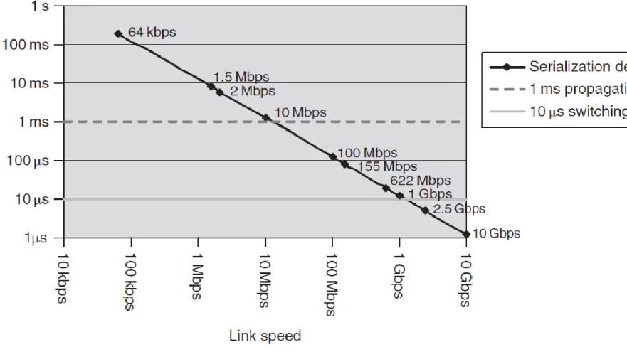
Serialization delay is the time taken to clock a packet onto a link and is dependent upon the link speed and the packet size.
Serialization delay is proportional to packet size and inversely proportional to link speed:
Serialization delay can generally be considered negligible at link speeds above 155 Mbps (e.g. STM-1/OC3) such as backbone links, but can be significant on low-speed links. The serialization delay for a 1500-byte packet at link speeds from 64 kbps to 10 Gbps is shown in Figure 1, together with a line plotting indicative switching delay and a line showing a propagation delay of 1 ms (e.g. a link distance of 130 km).
4 Serialization Delay
Delay-jitter
Delay-jitter characterizes the variation of network delay. Jitter is generally considered to be the variation of the one-way delay for two consecutive packets, as defined by [RFC3393] in the IETF. In practice, however, jitter can also be measured as the variation of delay with respect to some reference metric, such as average delay or minimum delay. It is fundamental that jitter relates to one-way delay; the notion of round-trip time jitter does not make sense.
Jitter is caused by the variation in the components of network delay:
Propagation delay. Propagation delay can vary as network topology changes, when a link fails, for example, or when the topology of a lower layer network (e.g. SDH/SONET) changes, causing a sudden peak of jitter.
Delay-jitter
Scheduling delay. Variation in scheduling delay is caused as schedulers’ queues oscillate between empty and full.
Serialization delay. Serialization delay is a constant and as such should not contribute to jitter directly. If during a network failure, however, traffic is rerouted over a link with a different speed, then the serialization delay will change as a result of the failure and the change in serialization delay may contribute to jitter.
Packet Loss
Packet loss characterizes the packet drops that occur between a defined network ingress point and a defined network egress point. A packet sent from a network ingress point is considered lost if it does not arrive at a specified network egress point within a defined time period.
A metric for measuring the one-way packet loss rate (PLR) has been defined by [RFC2680] in the IETF.
One-way loss is measured rather than round-trip loss because the paths between a source and destination may be asymmetrical; that is, the path routing or path characteristics from a source to a destination may be different from the path routing or characteristics from the destination back to the source. Round-trip loss can be estimated by measuring the loss on each path independently.
Packet Loss
Consequently, [RFC3357] introduces some additional metrics, which describe loss patterns:
“loss period” defines the frequency and length of loss (loss burst) once it starts; “loss distance” defines the spacing between the loss periods.
Packet loss can be caused by a number of factors:
Congestion. When congestion occurs, queues build up and packets are dropped. Loss due to congestion is controlled by managing the traffic load and by applying appropriate queuing and scheduling mechanisms.
Packet Loss
In practice, actual bit error rates (BER, also referred to as the bit error ratio) vary widely depending upon the underlying layer 1 or layer 2 technologies used, which is different for different parts of the network:
Fiber-based optical links may support bit error rates as low as to 1 * 10^(-13); Synchronous Digital Hierarchy (SDH) or Synchronous Optical Network (SONET)
services typically offer BER of 1 * 10(-12);
Typical E1/T1 leased line services support BER of 1 * 10(-9);
The Institute of Electrical and Electronics Engineers (IEEE) standard for local and metropolitan area networks [802-2001] specifies a maximum BER of 1 * 10(-8); Typical Asynchronous Digital Subscriber Line (ADSL) services support BER of 1 *
10(-7);
Satellite services typically support BER of 1 * 10(-6).
Packet Loss
Network element failures. Network element failures may cause packets to be dropped until connectively is restored around the failed network element. The resulting loss period depends upon the underlying network technologies that are used.
With a “plain” IP (i.e. non-MPLS) deployment, after a network element failure, even if there is an alternative path around the failure, there will be a loss of connectivity which causes packet loss until the interior gateway routing protocol (IGP) converges. In welldesigned networks, the IGP convergence time completes in a few hundred milliseconds. If there is not an alternative path available then the loss of connectivity will persist until the failure is repaired. While such outages could be accounted for by the defined loss rate for the service, they are most commonly accounted for in the defined availability for the service.
Where an alternate path exists, the loss of connectivity following network element failures can be significantly reduced through the use of technologies such as MPLS Traffic Engineering (TE) Fast Reroute (FRR) [RFC4090] or IP Fast Reroute (IPFRR), which are local protection techniques that enable connectivity to be rapidly restored around link and node failures, typically within 50 ms. Equivalent techniques may be employed at layer 2, such as
Packet Loss
Loss in application end-systems. Loss in application end-systems can happen due to overflows and underflows in the receiving buffer. An overflow is where the buffer is already full and another packet arrives, which cannot therefore be enqueued in the buffer; overflows can potentially impact all types of applications. An underflow typically only impacts real-time applications, such as VoIP and video, and is where the buffer is empty when the codec needs to play out a sample, and is effectively realized as a “lost” packet. Loss due to buffer underflows and overflows can be prevented through careful design both of the network and the application end-systems.
Bandwidth and Throughput
IP services are commonly sold with a defined “bandwidth,” where the bandwidth often reflects the layer 2 access link capacity provisioned for the service; however, when used in the context of networking the term “bandwidth” – which was originally used to describe a range of electromagnetic frequencies – can potentially have a number of different meanings with respect to the capacity of a link, network or service to transport traffic and data. Hence, to avoid confusion we define some more specific terms:
Link capacity. The capacity of a link is a measure of how many bits per second that link can transport; link capacity needs to be considered both at layer 2 and at layer 3.
The capacity of a link is normally constant at layer 2 and is a function of the capacity of the physical media (i.e. the layer 1 capacity) and particular layer 2 encoding used. Some media, however, such as ADSL 2/2 are rate-adaptive, and hence the layer 1 capacity can vary with noise and interference.
Bandwidth and Throughput
Class capacity. Where QOS mechanisms are used, an aggregate traffic stream may be classified into a number of constituent classes, and different QOS assurances may be provided to different classes within the aggregate. Where a class has a defined minimum bandwidth assurance, this is referred to as the class capacity, and may also be known as the class bandwidth.
Path capacity. Path capacity is the minimum link capacity on a path between a defined network ingress point and a defined network egress point, consisting of a number of links interconnected by a number of nodes or routers. also provides definitions for link and path capacity. Path capacity may also be referred to as the path bandwidth.
Bandwidth and Throughput
“Congestion aware” in this context refers to a transport layer technology that adapts its rate of sending, depending upon what is actually received, in order to try to maximize throughout; a TCP session is an example of such a congestion-aware transport layer connection.BTC is clearly limited by the path capacity, but is also impacted by a number of other factors such as packet loss and RTT, hence it is important to note that the BTC may be significantly lower than the link capacity specified in the SLA. BTC is a representation of the “goodput” available to a user, where the goodput represents the usable portion of the attainable throughput between a source and destination.
BTC is not applicable to non congestion-aware, i.e. non-adaptive or inelastic, services; for such services, their attainable throughput may not be a meaningful metric, but nonetheless may be derived from the path capacity and the loss rate commitments for the service.
Layer 2 Overheads
When considering the capacity of a service the available IP capacity depends upon the layer 2 media, the layer 2 encapsulation used and upon the layer 3 packet sizes. Different layer 2 encapsulations add different sized headers and trailers to each packet; the headers and trailers are an overhead from the perspective of IP services, in that they use available layer 2 capacity, which is therefore not available at layer 3.
As the layer 2 headers and trailers are added to each IP packet, the amount of layer 2 overhead incurred, and hence the IP capacity available, is dependent upon the IP packet size.
Layer 2 Overheads
Layer 2 Overheads
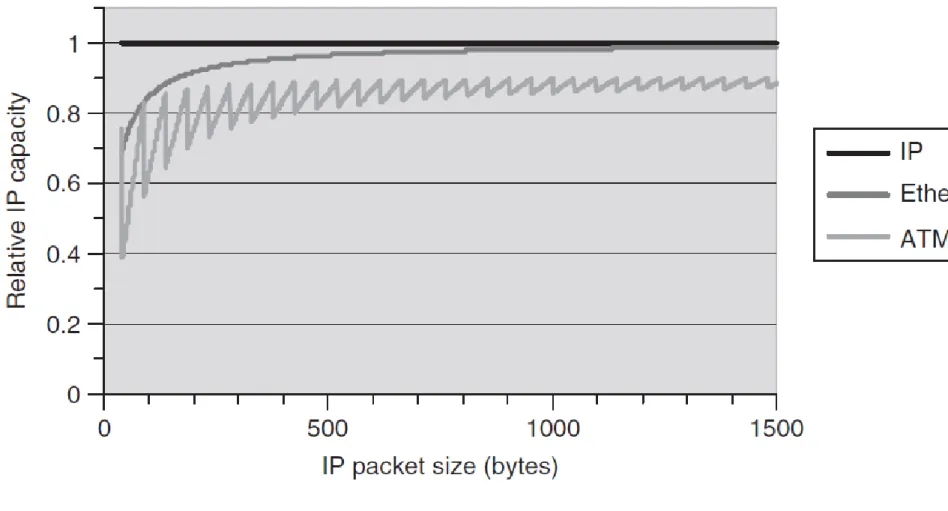
As can be seen from Figure 2, the available IP capacity can vary significantly depending upon the overall layer 2 overhead.
For Ethernet, the layer 2 overhead in bytes per IP packet is constant, irrespective of the packet size; hence the layer 2 overhead reduces relative to the available IP capacity as the IP packet size increases.
This is not the case for ATM, where an IP packet is segmented into cells and the per cell overhead or “cell tax” depends upon the number of cells, which in turn depends on the packet size. Hence, although the trend in the layer 2 overhead is to reduce relative to the available IP capacity as the IP packet size increases, a one-byte increase in packet size can result in an additional ATM cell, which results in an increase in the relative overhead; hence the saw tooth IP capacity characteristic for ATM in Figure 2.
Layer 2 Overheads
Consider for example, a simple two-queue (where a queue is ostensibly a class) scheduler with per-queue minimum bandwidth assurances defined at layer 3 of
X=Y=50%. With IP packet sizes of 100 bytes for queue X and 1000 bytes for queue Y, and
assuming a layer 2 overhead of 26 bytes per packet (as is the case with Ethernet v2), the measured bandwidth ratio X : Y at layer 3 is
(10 *100) : (1*1000)=50 : 50,
whereas the ratio measured at layer 2
(10 *126) : (1*1026)=55 : 45.
Conversely, assuming the same packet sizes and overhead but with per-queue minimum bandwidth assurances of X=Y=50% defined at layer 2, the resulting bandwidth ratio at layer 3
Layer 2 Overheads
In some cases, there are constraints imposed by the underlying layer 1 and layer 2 technologies, which naturally define the overheads that are taken into account in a particular SLA definition. In other cases there may be no definitive answer as to whether layer 2 overheads should be taken into account:
Accounting for all layer 2 overheads in actual router implementations can be difficult when, for example, layer 2 fragmentation mechanisms insert additional bytes after a packet has been enqueued.
Some service SLAs are defined excluding layer 2 overheads; while others to take layer 2 overheads into account; there is no de facto industry approach.
The IETF’s Integrated Services (Intserv) and Differentiated Services (Diffserv) architectures do not discuss or define the accounting of layer 2 overheads.