INITIAL ORBIT DETERMINATION ERROR ANALYSIS OF LOW-EARTH ORBIT ROCKET BODY DEBRIS AND FEASIBILITY STUDY FOR DEBRIS
CATALOGUING FROM ONE OPTICAL FACILITY
A Thesis presented to
the Faculty of California Polytechnic State University, San Luis Obispo
In Partial Fulfillment
of the Requirements for the Degree Master of Science in Aerospace Engineering
by Kyle Stoker
ii
© 2020
Kyle Stoker
iii
COMMITTEE MEMBERSHIP
TITLE: Initial Orbit Determination Error Analysis of
Low-Earth Orbit Rocket Body Debris and
Feasibility Study for Debris Cataloguing from
One Optical Facility
AUTHOR: Kyle Stoker
DATE SUBMITTED: June 2020
COMMITTEE CHAIR: Kira Abercromby, Ph.D.
Professor of Aerospace Engineering
COMMITTEE MEMBER: Eric Mehiel, Ph.D.
Associate Dean for Diversity and Student Success
COMMITTEE MEMBER:
COMMITTEE MEMBER:
Pauline Faure, Ph.D.
Assistant Professor of Aerospace Engineering
Morgan Yost, M.S.
iv
ABSTRACT
Initial Orbit Determination Error Analysis of Low-Earth Orbit Rocket Body Debris and
Feasibility Study for Debris Cataloguing from One Optical Facility
Kyle Stoker
This paper is predicated on determining the effectiveness of angles-only initial orbit determination (IOD) methods when limited observational data is available for low-Earth orbit (LEO) rocket body debris. The analysis will be conducted with data obtained from Lockheed Martin Space’s Space Object Tracking (SpOT) facility, focusing on their observational data from 2018 that contains tracking of rocket body debris for less than one minute per overhead pass. After the IOD accuracies are better understood, a feasibility study will follow that investigates the possibility of cataloguing LEO orbital debris from a single optical observation facility with similar observational capabilities as that of the SpOT facility.
v
ACKNOWLEDGMENTS
Special thanks to my graduate advisor Dr. Kira Abercromby for her support and
guidance throughout this whole project. Additionally, thank you to my whole committee
for assisting in whatever capacity required. I sincerely appreciate all of the assistance that
was provided, as it was invaluable in helping shape this project for the better.
Thank you to Lockheed Martin Space, and specifically everyone at the SpOT
Facility, whose efforts allowed this project to come together in the first place. The work
done in this paper would not have been possible without the data provided, and I hope
that the results of this research can help potentially shape more work on the subject
matter.
Thank you to my fiancée Georgina Plested, who helped keep me motivated to
work when I hit roadblocks along the way. Finally, thank you to my family, whose efforts
vi
TABLE OF CONTENTS
Page
LIST OF TABLES ... viii
LIST OF FIGURES ... x
LIST OF NOMENCLATURE ... xii
LIST OF SYMBOLS ... xiii
CHAPTER 1. INTRODUCTION ... 1
1.1 Preface ... 1
1.2 Purpose of Study... 3
1.3 Structure of Paper ... 7
2. BACKGROUND ... 9
2.1 Initial Orbit Determination Methods ... 9
2.2 Orbital Elements and Observation Angles ... 14
2.3 Space Debris ... 21
2.4 Optical Orbit Determination ... 23
2.5 SpOT Facility ... 31
3. METHODOLOGY ... 33
3.1 SpOT Facility Data Collection ... 33
3.2 Gaussian IOD ... 36
3.3 TLE Comparison and STK ... 43
3.4 Data Processing ... 47
3.5 Three-Point IOD ... 50
3.6 Iterative Approach ... 51
3.7 Assumed-Circular Orbit IOD... 54
3.8 Instrument Error ... 57
3.9 Lambert’s Problem ... 61
4. RESULTS AND DISCUSSION ... 65
vii
4.2 Reliability of Data and Gauss IOD ... 67
4.3 Three-Point IOD ... 70
4.4 Iterative IOD ... 79
4.5 Pointing Error Iterative IOD ... 84
4.6 ACO IOD ... 89
4.7 IOD Accuracy Comparison (Summary) ... 95
4.8 Feasibility of Subsequent Target Acquisition ... 96
4.8.1 Test Case 39 ... 96
4.8.2 Test Case 22 ... 103
4.8.3 Feasibility Discussion ... 107
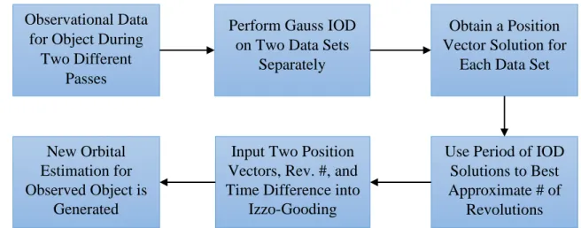
4.9 Multi-Rev Lambert’s IOD Improvement ... 111
5. CONCLUSION ... 114
6. FUTURE WORK ... 116
6.1 Comparison with Alternative IOD Methods ... 116
6.2 Orbit Determination System Creation ... 116
6.3 Expanding the Observed Object List ... 117
6.4 Performing IOD for Different Orbital Arc Periods ... 117
BIBLIOGRAPHY ... 119
APPENDICES A. Rocket Body Characteristics for STK Propagation ... 122
viii
LIST OF TABLES
Table Page
2.1. Completeness of SCC in 1990 from GEODSS Observations ... ...25
2.2. Summary of SpOT Performance in 2018 ... 32
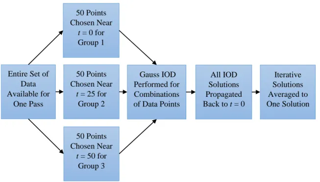
3.1. Grouping of Data for Iterative IOD Scheme ... ...54
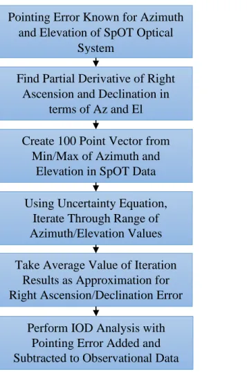
3.2. Pointing Error in Right Ascension and Declination... 60
4.1. Overview of Observational Data ... 66
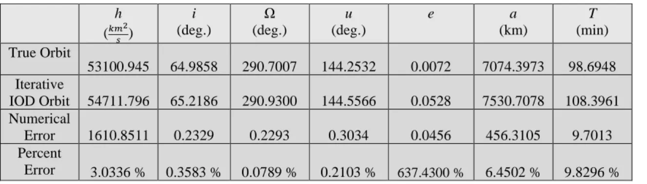
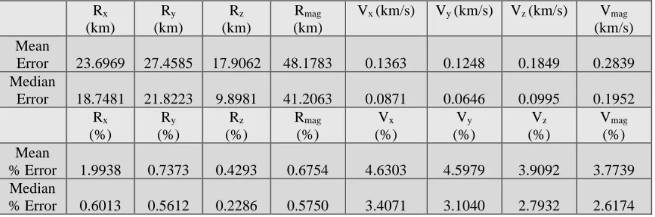
4.2. Three-Point IOD State Error ... 71
4.3. Three-Point IOD Orbital Elements Error ... 72
4.4. Test Case 18 Three-Point IOD Results ... 73
4.5. Test Case 14 Three-Point IOD Results ... 76
4.6. Iterative IOD State Error ... 80
4.7. Iterative IOD Orbital Elements Error ... 80
4.8. Test Case 18 Iterative IOD Results ... 81
4.9. Test Case 14 Iterative IOD Results ... 82
4.10. Positive Bias Iterative IOD State Error ... 85
4.11. Negative Bias Iterative IOD State Error ... 85
4.12. Positive Bias Iterative IOD Orbital Elements Error... 86
4.13. Negative Bias Iterative IOD Orbital Elements Error ... 86
4.14. ACO IOD State Error ... 90
4.15. ACO IOD Orbital Elements Error ... 90
ix
4.17. Test Case 18 ACO IOD Results ... 92
4.18. Test Case 3 ACO IOD Results ... 93
4.19. IOD Accuracy Comparison ... 95
4.20. Test Case 39 IOD Accuracies ... 97
4.21. Improvement in Accuracy Using Izzo-Gooding (Test Cases 1 and 2) ... 112
4.22. Improvement in Accuracy Using Izzo-Gooding (Test Cases 3 and 4) ... 112
A.1. Rocket Body Debris Upper Stage Characteristics ... 122
B.1. Three-Point IOD State Vector Errors ... 124
B.2. Three-Point IOD Orbital Element Errors ... 125
B.3. Iterative IOD State Vector Errors ... 126
B.4. Iterative IOD Orbital Element Errors ... 127
B.5. Iterative (Negative Bias) IOD State Vector Errors ... 128
B.6. Iterative (Negative Bias) IOD Orbital Element Errors ... 129
B.7. Iterative (Positive Bias) IOD State Vector Errors ... 130
B.8. Iterative (Positive Bias) IOD Orbital Element Errors ... 131
B.9. Assumed-Circular Orbit IOD State Vector Errors ... 132
x
LIST OF FIGURES
Figure Page
2.1. Three Distinct Observations Required for Initial Orbit Determination ... 10
2.2. Subset of Orbital Elements ... 15
2.3. Azimuth and Elevation Angles ... 19
2.4. Right Ascension and Declination Angles ... 20
2.5. Space Debris Accumulation Over Time ... 21
3.1. SpOT Data Acquisition and Transfer to Cal Poly ... 35
3.2. TLE Format and Structure ... 44
3.3. Overview of TLE Orbital Element Retrieval in STK ... 46
3.4. Unfiltered Observation Data for R/B 00694 ... 49
3.5. Summary of Iterative IOD Scheme ... 54
3.6. Summary of ACO IOD Scheme ... 57
3.7. Telescope Pointing Error Methodology Summary ... 61
3.8. Summary of Izzo-Gooding and Multi-Revolution Methodology ... 64
4.1. Test Case 13 Propagated Orbit Solution ... 67
4.2. Test Case 13 Right Ascension and Declination Angles ... 68
4.3. Test Case 18 Three-Point IOD Orbital Plot Comparison ... 74
4.4. Test Case 18 Three Point IOD Observational Angles Over Time ... 75
4.5. Test Case 14 Three-Point IOD Orbital Plot Comparison ... 77
4.6. Test Case 14 Three Point IOD Observational Angles Over Time ... 78
xi
4.8. Test Case 14 Iterative IOD Observational Angles Over Time ... 83
4.9. Three Iterative Scheme Solutions for Test Case 11 ... 87
4.10. Three Iterative Scheme Solutions for Test Case 45 ... 88
4.11. Test Case 18 ACO IOD Observational Angles Over Time ... 93
4.12. Test Case 3 ACO IOD Observational Angles Over Time ... 94
4.13. Test Case 39 Right Ascension and Declination Over Time ... 98
4.14. Test Case 39 Shared Observation Angle Trends ... 100
4.15. Error Between Telescope Pointing Direction and Observed Object ... 101
4.16. Test Case 39 Observation Angles Compared to Field of View Limitation ... 102
4.17. Test Case 22 Right Ascension and Declination Over Time ... 103
4.18. Test Case 22 Observation Angles Compared to Field of View Limitation ... 104
4.19. Test Case 22 Observational Angle Error with Expanded Field of View ... 105
xii
LIST OF NOMENCLATURE
Abbreviation Full Meaning
ACO Assumed-Circular Orbit
AGI Analytical Graphics, Inc.
DOMES Distributed Observatory Manager for Enhanced SSA
ECI Earth Centered Inertial
FoV Field of View
GEO Geosynchronous Orbit
GEODSS Ground-Based Electro-Optical Deep Space Surveillance
GTO Geosynchronous Transfer Orbit
IOD Initial Orbit Determination
JSC Johnson Space Center
LEO Low-Earth Orbit
LLA Latitude, Longitude, and Altitude
MATLAB Matrix Laboratory
MODEST Michigan Orbital Debris Survey Telescope
NaN Not a Number
NORAD North American Aerospace Defense Command
R/B Rocket Body
RAAN Right Ascension of Ascending Node
RSO Resident Space Object
SCC Space Command Catalog
SGP4 Simplified General Perturbations Model
SpOT Space Object Tracking
SDA Space Domain Awareness
SSN Space Surveillance Network
STK Systems Tool Kit
xiii
LIST OF SYMBOLS
Symbol Meaning Units
𝐴𝑧 Azimuth Angle degrees
El Elevation Angle degrees
𝑅⃗ Site Vector km
Rmag Magnitude of Position Vector km
Rx X-Position km
Ry Y-Position km
Rz Z-Position km
T Period minutes
Vmag Magnitude of Velocity Vector km s⁄
Vx X-Velocity km s⁄
Vy Y-Velocity km s⁄
Vz Z-Velocity km s⁄
a Semi-major axis km
e Eccentricity ---
f, g Lagrange Coefficients ---
h Angular Momentum km2⁄s
i Inclination degrees
q Uncertainty Value ---
𝑟⃑ Position Vector of Object km
𝑡𝑖 Time at ith Observation Point seconds
u Argument of Latitude degrees
𝑣̂ Velocity Unit Vector ---
𝑣⃑ Velocity Vector km s⁄
Ω Right Ascension of Ascending Node degrees
α Right Ascension Angle degrees
δ Declination Angle degrees
θ True Anomaly degrees
𝜇 Gravitational Parameter of Earth km3⁄s2
ρ Slant Range Magnitude km
𝜌̂ Slant Range Unit Vector ---
𝜑 Latitude degrees
1 Chapter 1 Introduction 1.1 Preface
The increasing number of objects in Earth-orbit over the last decade has placed an
emphasis on having up-to-date coverage and tracking of debris in space, as the risk of
collision between objects can be minimized through knowledge of the constantly
evolving debris environment. While operational spacecraft can utilize their onboard
electronics to aid in their orbit determination processes, debris tracking requires the use
of ground-based radar or optical observation facilities to obtain data that can be used in
determining the orbital parameters of debris.
The United States operates the Space Surveillance Network (SSN), whose
combination of optical and radar telescopes allow for around the clock data collection for
spacecraft and debris. With more than 20 facilities across the globe, the SSN is capable of
observing objects at a multitude of orbital altitudes and locations around Earth [14]. The
data collected on orbiting objects is used to maintain an up-to-date awareness of where
objects are at any current time, as well as their predicted location in the future.
The most common public source for orbital information on any tracked object is
the two-line element (TLE) sets posted online for every object that is tracked and
catalogued by the SSN. These succinct descriptions of an object’s orbital parameters at a
certain time stamp are frequently updated and kept up to date with new observational data
from the SSN when available [14]. While these TLE sets are provided to the public, not
2
The orbital model used in generating TLE sets is the Simplified General
Perturbations (SGP4) model, and the code that runs this has been published into the
public domain. The SGP4 orbital model used by the United States Department of Defense
has been updated since its original publication in 1980, and these changes, although not
comprehensively re-released by the Department of Defense, have been studied and
amended through independent study into the SGP4 orbital model [31]. It is important to
note that all propagation of a TLE data set should use the SGP4 model in order to
maintain the highest level of accuracy, as it is the same model that is used in creating the
TLE data. Using any other propagator would create an inconsistency in the orbital
modeling and result in errors when propagating an object’s orbit forward in time.
The orbit determination algorithms that go into creating TLE sets, however, are
not available to the public. These algorithms are used with the observational data in order
to estimate an object’s orbital path, and these algorithms can incorporate new data as it
becomes available, allowing for updated TLE sets to be posted regularly. TLE sets are
generally accurate to approximately one kilometer for the epoch time at which they are
posted [32], but this can vary for different objects depending on many factors, including
quantity of observational data, quality of the observation equipment, and the type of orbit
the object is in [14]. While tracked objects (greater than 10 cm in diameter for LEO, 1
meter in GEO) have well-understood orbits due to observational data being obtained
regularly, objects that are untracked will have no data in which to base an orbital estimate
on. This leads to uncertainty in orbital accuracy when trying to estimate an object’s orbit
for the first time, and without access to either the data or the algorithms that help create
3
When attempting to identify, track, and catalog an unidentified debris object,
there will be no a priori information available on which to base any orbit determination
calculations upon. Thus, any initial orbit determination process will need to produce
results that are accurate enough to allow for the object to be found again in successive
passes, wherein the initial orbit determination results can be refined and improved upon
further.
For low-Earth orbit (LEO) objects, visible passes only last around 10-15 minutes
during a direct overhead pass, and can be much shorter during sub-optimal conditions
where the object does not pass directly overhead. Additionally, time must be allocated to
find an object, track it overhead, and begin collection of data. This results in actual
observational data on the scale of a few minutes at most. When compared to orbital
period of LEO objects, which average approximately 90-100 minutes [30], the orbital arc
observed during any one observational period encompasses only a small fraction of the
entirety of the orbit. This makes LEO object orbit determination especially difficult as
compared to other orbital regimes.
1.2 Purpose of Study
To better understand the accuracies one can expect when performing initial orbit
determination for a LEO object, a study will be performed using observational data from
Lockheed Martin Space’s Space Object Tracking (SpOT) facility, focusing primarily on
their observations of rocket body debris in 2018. The choice of rocket bodies as the
studied object, and more detailed information about the SpOT facility, will be discussed
4
In order to understand the inherent error present in an initial orbit determination
solution, a true orbital solution must be known and used as comparison. The baseline
solution will be historical TLE data for the observed rocket bodies, whose orbital
ephemeris can be propagated to the observation times and directly compared in terms of
its orbital state and elements. While there will be no comparative benchmark in which to
qualify results when attempting to analyze untracked debris, it is a necessary comparative
tool in order to better understand the accuracy one can expect from an initial orbit
determination solution. Once this expected accuracy is better understood, this knowledge
can be applied to situations where there is no TLE data to reference, and can help assist in
the observation and tracking of uncatalogued debris.
After an understanding of expected IOD errors is formed based on the analysis of
rocket body debris, a feasibility study will follow that looks into the possibility of one
optical facility having the capability of observing and cataloguing unknown debris
objects. As mentioned in the preface, this task is normally accomplished by the SSN,
which has numerous facilities and many resources at their disposal to keep track of the
objects in space. Being able to perform a similar function with only one optical facility,
and making the gathered results and procedural methods directly available to the public,
would benefit the overall knowledge of the space environment.
In pursuing the goal of better characterizing the accuracy of initial orbit
determination and analyzing the feasibility of an optical facility’s ability to observe
untracked debris in the future, some general project goals were developed in order to
5
1. Developing the code to perform orbit determination to a high degree of accuracy
In order to achieve the goal of performing an accuracy analysis of initial orbit
determination for LEO debris, IOD algorithms and procedures will need to be
developed, tested, and validated. For the purposes of quantifying the accuracy of
initial orbit determination, the IOD orbital solutions will be compared to historical
TLE data for the rocket bodies, which will be treated as the true orbit of the
observed debris object. The error between each IOD solution and the true orbit of
the object will then be used to analyze the accuracy of the IOD solution by
propagating the solution forward in time, comparing the orbital elements and
observation angles in the future. This will lead directly into the feasibility of
cataloguing debris, which is further explained in the fourth project goal.
Many different functions are required to perform orbit determination, and thus all
these functions must be thoroughly reviewed to ensure there are no errors that
could cause illegitimate results. The development of these procedures and all code
written are completed in MATLAB R2016b. The majority of the functions used
are the author’s own work, while any supplementary functions that are not will be
clearly identified and referenced.
2. Identifying, through testing, the best method to maximize the effectiveness of the data provided by the SpOT facility
As mentioned in the preface, LEO debris observations are very short in duration.
Specifically speaking on the rocket body debris data collected in 2018 from the
6
approximately one minute long. Because there is no means to obtain more
observational arc from this data, the focus must shift to maximizing the
effectiveness of short arc observations in order to accurately depict the entire orbit
of an object. Multiple different methods will be discussed and analyzed
throughout this paper as an attempt to maximize the efficacy of the data, including
traditional three-point IOD, an iterative approach, and an assumed-circular orbit
(ACO) approach.
3. Analyzing the error in orbit estimation from the applied IOD methods
Through the data transfer from the SpOT facility to Cal Poly, a large quantity of
observational data was made available for use in this paper. Out of this data, a
large subset falls within the range of 50 to 60 seconds of observational coverage
per pass, with the rest of the data below the 50 second threshold. The analysis of
orbit determination error will be focused on the 50 to 60 second subset, as this
data group exemplifies the optical capabilities of the SpOT facility with regard to
rocket body debris coverage in 2018. Additionally, this data has the maximum
observation time per pass of the available data, and will theoretically yield the
most accurate results due to the larger orbital arc that is covered by this data.
Each of the aforementioned initial orbit determination approaches (three-point,
iterative, ACO) will be applied to each pertinent data set. The respective errors for
specific passes, as well as a total average and median error, can be computed and
quantified for each method. This will allow for direct comparison between each
orbit determination method, and ultimately give insight into which method
7
4. Determining the feasibility of using short-arc optical data as a means to characterize and catalog untracked orbital debris in LEO
After the analysis of orbit estimation error has been finished, a feasibility study
will be conducted on the IOD results. This will delve into the specific errors in the
IOD solutions for all data sets, and look at the feasibility of utilizing an optical
facility such as SpOT for future cataloguing of orbital debris. The main question
looking to be answered in this portion of the paper will be: Are the initial orbit
determination solutions of rocket bodies accurate enough for the object to be
observed on subsequent passes, allowing for the object’s orbital solution to be
further refined towards ultimately being added to the catalog of known space
debris? If the answer is yes, further investigation towards attempting to catalog an
unknown object with a system such as SpOT can be undertaken. If the answer is
no, more analysis will need to be conducted to find what changes can be made to
an optical observation system to allow for this goal to be achieved, or it may be
deemed currently infeasible with current technology.
Through the accomplishment of these project goals, IOD accuracies for LEO
debris can be characterized, and the feasibility of using angles-only orbit determination
techniques to catalog LEO debris will be better understood. The next section will give a
brief overview of the layout of this thesis document, and how the future chapters will be
structured.
1.3 Structure of Paper
This section will conclude Chapter 1, which gave a little bit of insight into why
8
paper. Background information, including information on topics such as traditional IOD
methods, the threat of space debris, similarly themed optical orbit determination projects,
and more detailed info on Lockheed Martin Space’s SpOT facility will follow in Chapter
2. Chapter 3 will dive into the methodology and some of the specific algorithms that were
implemented as part of this thesis in order to achieve the project’s goals. Chapter 4 will
introduce the results of the project, with graphical and tabular results highlighting the
section. These results will be accompanied by discussion on the results and how they
relate to the goals of the project. Chapter 5 will include a summary of this project’s
findings, and Chapter 6 will include some potential projects and future work that can
9 Chapter 2 Background
Before discussing the specific work and results of this paper, it is important to
understand some background information on the topic of initial orbit determination and
why space debris is an important topic of study, as well as review some similar projects
that have been conducted in this area of research. The first section will give a synopsis of
IOD methods and how their application to observational data allows for an object’s orbit
to be estimated.
2.1 Initial Orbit Determination Methods
Obtaining a first estimation of an object’s orbital parameters requires solving for
six independent quantities. This can be expressed in terms of the classical orbital
elements (inclination, right ascension of ascending node, eccentricity, true anomaly,
argument of periapsis, and semi-major axis), or in terms of a state vector with radius and
velocity vectors (Rx, Ry, Rz, Vx, Vy, and Vz). Optical telescopes are able to provide only
two independent quantities for a single observation: right ascension and declination. With
only two values and six unknown quantities to solve for, three distinct observations of an
object must be made to perform initial orbit determination [8]. A visual description of
this can be seen on Figure 2.1.
On Figure 2.1, C represents the center point of Earth, from which two different
types of position vectors extend. R1-3 represent the site vectors, which are the position
vectors of the observation location on Earth’s surface at t1-3, the three observations times.
r1-3represents the position vectors of the actual orbiting object with respect to the center
10
denoted as ρ1-3, is the position vector that extends from the observation location O to the
observed object at each observation time. Finally, the velocity vector v2depicts the
velocity of the orbiting object with respect to Earth’s center, C. Out of these variables, the
only known values before observation are the site vectors at each observation time and
the exact time at which each observation takes place. The slant range, position vector of
the observed object, and the velocity vector of the observed object are unknowns that
must be solved for in order to generate an initial orbit determination.
Figure 2.1: Three Distinct Observations Required for Initial Orbit Determination [8]
The major distinction between angles-only IOD and the other main form of
observational orbit determination, radar IOD, is the lack of data regarding the slant range
and the range rate. Radar observations provide the user with information about both the
11
overhead during observation. Angles-only optical observations are thus tasked with
solving for the slant range using only the output of look angles from the telescope. After
solving for the slant range, position vectors can be calculated through addition of the site
vector and the slant range vector for each observed location. With these values found, a
velocity vector can be calculated at the middle observation point using the position
vectors at each of the three observation times. A more detailed explanation of the
angles-only IOD methodology used in this paper will occur in Section 3.2.
There are multiple different optical IOD methods that have been developed in the
past for use with angles-only input data. Some of these methods include Gaussian IOD,
Double-R IOD iteration, and Gooding IOD. These three methods were considered for use
in this paper due to their differing strengths and weaknesses with regard to initial orbit
determination, with each method presenting different advantages depending on the work
being performed. The benefits and limitations of each of these methods were investigated
in order to decide which method best aligned with the goals of this project.
Gauss’ method was originally applied to interplanetary studies of orbiting bodies,
but has more recently been used in satellite orbit determination. For IOD of
Earth-orbiting objects, this method is most accurate when the angular separation between
observations is small, with less than 10 degrees of separation between observations being
optimal. On a timescale, this translates to observations that are around 5 to 10 minutes
apart for LEO objects. One limitation of the Gauss IOD method is that it can suffer from
singularity issues when the observed line-of-sight vector lies in the same plane as the
observed object’s orbital plane [11]. The Gauss IOD method also requires that the roots
12
the range estimate for the object. While this method is limited to use with closely spaced
data, its formulation lends itself to be a fairly robust way to initially determine an object’s
orbit given angles-only data [33].
The Double-R IOD method is a combination of numerical and dynamical
techniques that helps solve for orbital parameters given angles-only data. This method,
contrary to the application of Gauss’ method, works most effectively for data that is
separated by large differences in orbital arc between observations. The Double-R method
has the benefit of being able to incorporate data that spans multiple days if observations
occur during one orbit of an observed object, but it is not capable of solving for a solution
if the data spans multiple revolutions [33]. For LEO observation, the Double-R method is
limited in its ability to produce accurate results, where the observations of an object are
likely to be separated by minutes at most. Additionally, the Double-R method requires
initial range estimates as inputs to the algorithm that are to be iterated upon, and if these
estimates are not close enough to the true solution, the method has a difficult time
converging to a meaningful solution [11].
The Gooding method builds upon the Double-R iterative method, but utilizes
Gooding’s own Lambert’s solution. The method is iterative, can solve for orbits of any
eccentricity, and works with data from multiple revolutions [33]. This is important for
when a pass of a LEO object lasts only a few minutes, limiting the time to obtain data
points from the ground. Being able to incorporate data from multiple passes makes the
Gooding method very robust and useful with almost any data set [33]. Although the
Gooding method is very useful in that it can incorporate a multi-revolution solution, it
13
Double-R, and struggles to converge to an accurate solution if this initial estimate is not
close to the true range of the object. The number of revolutions between observations
must be specified as an input as well, so this value must be known in order to obtain
accurate results for an object’s orbit. Lastly, the Gooding method can yield multiple
solutions, so deciding which of the solutions is suitable for the input data can prove
difficult, especially when the target object’s orbit is unknown to the observer [11].
The benefits and limitations of these three methods were all considered in
choosing the most appropriate method to use alongside the data provided by SpOT to
analyze initial orbit determination accuracies. Given that each pass from the SpOT
dataset lasts at most 1 minute in duration, Gauss IOD was deemed more appropriate than
Double-R in creating an accurate initial orbit determination due to its success with
closely grouped data points. While the Gooding method has the strong advantage of
being capable of incorporating multiple revolutions worth of data, this will not be
applicable initially when only one pass of data is available for a debris object. Thus, the
major strength of the Gooding method would not be of benefit in achieving the goals of
this paper, and the method would still require the initial estimate of range to be accurate
enough to allow for convergence to a solution. For these reasons, Gauss IOD was chosen
as the primary IOD method in which the analysis of this paper will be founded.
Gauss IOD performs with inputs of three observational points, but being able to
include more than three points can help in refining the accuracy of an IOD solution from
one pass of observational data [33]. For any one pass of data for the rocket body debris
that will be analyzed in this paper, hundreds and sometimes thousands of observational
14
each object. Only using three of these data points can provide a reasonable estimate for
an object’s orbit, but incorporating many of these points can potentially increase the
accuracy of the IOD results. In order to include more than just three data points for each
data set available, an iterative approach and an iterative assumed-circular orbit approach
will be used that iterate on multiple data points using the Gauss IOD method in pursuit of
better estimating the observed object’s orbit. These methods will be further developed in
the methodology section of this paper, and compared with the baseline Gauss IOD results
from only using three points in generating an initial orbit determination.
Throughout the Results and Discussion section of this paper, the orbital solutions
will be presented and compared with regards to their state vector (position and velocity)
as well as their orbital elements. The next section will introduce all of the relevant orbital
elements that will be used as a comparative tool for analysis later on in the paper.
Additionally, the next section will define the observational look angles of right ascension
and declination, as well as azimuth and elevation, which will be referenced throughout
the paper.
2.2 Orbital Elements and Observation Angles
Orbital elements are often used to describe an object’s orbit, as they allow for a
generic and universal way to understand what type of orbit an object is in. There are
many different ways to express the orbital parameters of an object, each requiring at least
six parameters to be defined. Some of the traditional orbital elements are depicted in
15
Figure 2.2: Subset of Orbital Elements [15]
One of the classical elements depicted above is inclination (i), which describes the
incline of the orbital path with respect to the plane of reference. This reference plane is
the x-y plane of an Earth Centered Inertial (ECI) celestial reference frame, which
correlates to the equatorial plane of Earth. The inclination is best defined as the tilt of the
orbital path, and is measured from the equatorial plane to the orbital plane at the point of
the ascending node, shown in Figure 2.2. Inclination is measured from 0 to 180 degrees,
where an orbit with either 0- or 180-degree inclination represents an equatorial orbit that
stays positioned over Earth’s equator for the entirety of its orbit. Any value in between
represents an inclined orbit of some magnitude. Orbits between 0- and 90-degrees
inclination are moving prograde with Earth, meaning that the object’s orbital path is
moving in the same direction as Earth’s rotation beneath it. From 90- to 180-degrees, the
orbit is considered retrograde, and the object is moving in the opposite direction of
Earth’s rotation below. Finally, an exact 90-degree inclined orbit represents a polar orbit,
16
Longitude of ascending node, often written as the right ascension of the ascending
node (RAAN or Ω), is the angle measured eastward from the reference direction to the
point of the ascending node. This reference direction in an ECI reference frame is the
directional vector pointing towards the First Point of Aries, or Vernal Equinox, and
defines the x-direction of the ECI frame. The ascending node is defined as the point at
which the orbit passes the equatorial plane from South to North, which gives the name
“ascending” node. RAAN can thus have values ranging from 0- to 360-degrees.
Argument of periapsis (ω) defines the angular value between the ascending node and the periapsis, which is the point at which the object is closest to Earth during its orbit.
True anomaly (θ) represents the angle between the location of periapsis and where the object currently is in its orbital path. Both of these values can be seen in Figure 2.2 as well.
Specific angular momentum (h) is often used as a classical orbital element when
describing the orbit of an object. Specific angular momentum refers to the angular
momentum of the object, but divided by the mass term that would normally be included
[33]. It is calculated using the following equation:
ℎ⃗⃑ = 𝑟⃑ 𝑥 𝑣⃑ (2.1)
where 𝑟⃑ and 𝑣⃑ are the position and velocity vectors of an orbiting object in an
Earth-centered inertial reference frame.
The eccentricity (e) of an object’s orbit determines how circular or non-circular
the orbital path is. Object’s with an eccentricity of zero are in a circular orbit, where the
positional magnitude of the object remains constant throughout the entire orbit.
17
a time of closest approach to Earth (periapsis) and a time of farthest approach to Earth
(apoapsis). Eccentricities above 1 depict hyperbolic orbits for objects that are unbounded
in the Earth system; these objects do not have orbits that remain within Earth’s sphere of
influence.
While these six values completely define an orbit, there are other variables that are useful for describing an orbit depending on the situation and specific characteristics of the orbit that are being discussed. Argument of latitude (u) is defined as the angle between the ascending node to the position of the object at a certain epoch. It is more easily written as the sum of true anomaly and argument of periapsis. Specifically with the analysis to come in this paper, comparing orbital solutions against one another by using solely ω and θ will be difficult, as it requires that the solution can solve for the exact position of periapsis of the orbit as compared to the real orbital solution. This can become difficult for orbits that are very close to circular, as a truly circular orbit has infinite points that can be defined as the point of periapsis. Argument of latitude is not limited by this factor, and will give a better representation of the IOD solutions accuracy as
compared to the true orbit of the observed object.
18
Lastly, the orbital period (T) is a measure of how long an object takes to complete one full revolution around Earth. Something that will become more apparent in the Results and Discussion section is the difficulty in calculating a highly accurate velocity vector using angles-only IOD methods, especially when the orbital arc covered by the observations is very small. If the calculated velocity at a certain epoch is too large in magnitude, it causes the orbital solution to have a larger orbit and thus a longer period than the true orbit. If the calculated velocity is too small in magnitude, the opposite effect is observed, and the period is shorter than the true orbit. This leads to period being a good means of comparison between an IOD and true orbital solution, especially when the goal is to be able to find an object again in the future at a specific time and place in the sky.
This top-level background on orbital elements covers the basis of what is needed to understand the comparative nature of the results that constitutes the foundation of this paper. Next, some background information on observational angles will be discussed, as they will be mentioned throughout this paper and are fundamental to the methodology of this research.
19
Figure 2.3: Azimuth and Elevation Angles [34]
Azimuth is defined clockwise from due north of the observation location, describing which direction the object is in the sky from this vector. Azimuth can have values from 0 degrees up to 360 degrees. Elevation defines the angle between the horizon and the line-of-sight angle of the observed object, and can have a value between 0 and 90 degrees [34]. These two angles, and the time at which the observation takes place, fully define where an object is located overhead at any single instance in time, and will be discussed further when looking at telescope pointing angle errors in Section 3.8.
20
Figure 2.4: Right Ascension and Declination Angles [8]
21
The next section will give a brief overview of the growing space debris problem, and some rationale behind choosing rocket debris as the test subject for this paper.
2.3 Space Debris
Since the launch of Sputnik in 1957, the number of objects in space has been
tracked and catalogued, allowing for a better understanding on a global viewpoint of
where all spacecraft and debris are located at any given time. Figure 2.5 shows the
accumulation of Earth-orbiting objects that have been tracked on a year-to-year basis
(greater than 10 cm in diameter for LEO, 1 meter in GEO).
Figure 2.5: Space Debris Accumulation Over Time [2]
The last ten years have seen an approximate doubling of the objects being tracked
in Earth-orbit, an alarming spike that has seen the total object count surpass 22,000 as of
2019 [2]. This presents a multitude of problems, mainly with the potential risk of
collisions between objects in space. Being able to accurately define the orbit of all debris
22
damage or destroy active spacecraft, and can potentially create hundreds of new pieces of
space debris as fallout of a collision.
When orbital collisions take place, such as the collision between Iridium 33 and
Cosmos 2251 in 2009 (approx. 2000 pieces of debris > 10 cm in diameter were created)
[24], tracking the fallout debris and resultant trajectories of all debris pieces that are
generated by the collision is essential. Limited data will be available on the debris, and
understanding the confidence to have in initial orbit determination results is an important
factor when looking at warning active satellites of collision probabilities and allowing
them time to perform an orbital maneuver to minimize the risk of collision [29].
Additionally, as the technology allows for it, smaller pieces of debris will be tracked and
catalogued. When getting initial data back on uncatalogued debris objects, it is important
to understand the accuracy of the orbit determination results based on your optical data
input.
Optical orbit determination techniques work in a similar manner regardless of the
object being observed, but the focus for the testing done in this paper will be rocket body
upper-stage debris in LEO. This is due to a few reasons. First, the large size of rocket
body debris makes them one of the easier groups of objects to observe from an optical
facility, lending to them being one of the more readily available sources of data for
debris. Next, rocket body debris is non-controlled, meaning that there is no chance that
the object will perform any controlled maneuver that would alter the orbit. This ensures
that the orbit determination methods that are used will not produce inaccurate results due
to corrective maneuvering of the object. Lastly, rocket body stages are tumbling objects,
23
observed with optical instrumentation [18]. Other groups of debris types are similarly in a
tumbling state, making rocket bodies a good representation of debris in general.
Analyzing rocket body debris will be representative of debris as a whole, and the results
obtained from performing orbit determination on rocket bodies will be directly relatable
to all debris types.
While steps are being taken to limit the potential harm of space debris, it is
impossible to completely eradicate the threat that all current debris pose to current and
future space operations. The growing amount of debris in orbit is a mounting problem
that needs to be well understood in order to preserve the future of space activity. Being
well prepared for debris-creating events when they occur is one of the best ways to
minimize the negative potential of the debris. The next section will discuss how systems
centered around optical observation and orbit determination have been used to study
space debris and increase our knowledge of the debris environment.
2.4 Optical Orbit Determination
Optical telescopes have been increasingly utilized in the application of spacecraft
and debris tracking in recent years. Due to their inherent design, optical telescopes can be
heavily affected by factors such as light pollution, weather, and atmospheric turbulence,
so observational locations are often chosen based on limiting the negative effects that
these factors can have.
For any optical instrumentation, observational times in LEO are limited to when
an object is sunlit and the observation location is dark, resulting in optical telescopes
working in conditions of astronomical twilight: 1 to 2 hours before dawn, and 1 to 2
24
well-studied since 1984 and thoroughly investigated over the past three decades, leading
to an increased knowledge of the debris environment in the LEO regime [27].
In 1990, the space science branch at Johnson Space Center (JSC) worked towards
improving the knowledge of orbital debris between the altitudes of 500 and 1100
kilometers, with a majority of their optical observational data gathered from their
Ground-Based Electro-Optical Deep Space Surveillance (GEODSS) telescopes in Maui,
Hawaii and Diego Garcia, British Indian Ocean Territory [10]. These telescopes have an
aperture of 1 meter, a field of view of 1.6 x 1.2 degrees, and a limiting magnitude of 16.0
for stationary images, which denotes the brightness of the faintest object that can be seen
by the telescope.
Observational data was acquired one hour prior to morning nautical twilight, with
5 minutes spent observing a standard star field, and the rest of the hour allocated to
pointing the telescope at the zenith. These data tapes were then analyzed to identify all
objects that passed through the field of view of the telescope, with a total of 80.9 hours of
search time included in the analysis [10].
Using the time, position angle, and the rate of motion of each object seen in the
data tapes, many of the objects could be identified based on the predicted look angles
when compared to the United States Air Force Space Command Catalog (SCC), a catalog
of all known objects in space. If an object did not match any predicted look angles of the
object’s in the SCC, the object was considered unidentified and not catalogued at the
time. In total, the GEODSS telescopes identified 622 Earth-orbiting objects, 2649
meteors, and 16 objects of uncertain identity over the approximate 81 hours of
25
One of the major findings of this project was that the SCC at the time was very
incomplete, specifically in the LEO region. The comparison of the GEODSS
observations compared to the Space Command Catalog is shown below in Table 2.1,
taken from the paper detailing the findings of their work [10].
Table 2.1: Completeness of SCC in 1990 from GEODSS Observations [10]
The comparisons are done for 200 km regions from 500 to 1100 km in altitude, as
well as for various sizes of object (10-30 cm, 30-100cm, 100-200cm, >200 cm in
diameter). Over the entire 500-1100 km range, the total completeness factor of the SCC
was only 46%, meaning that only 46% of the objects seen by the GEODSS observations
26
were uncatalogued and not being tracked at the time. While 87% of objects between
100-200 cm and 78% of objects greater than 100-200 cm were successfully identified using the
SCC, a mere 26% of objects between 10 and 30 cm were a part of the catalog. The
research done by JSC at the time highlighted a very large discrepancy between the
catalogued debris and the actual amount of debris in orbit, and a lot of work has been
done since 1990 to narrow this discrepancy.
A more recent project was investigated in 2006 using the Michigan Orbital Debris
Survey Telescope (MODEST) telescope in Chile, focusing on the feasibility of
performing a survey of the GEO regime followed by immediate tracking of the objects
surveyed to obtain more precise orbital parameters of the debris [1]. Tracking of objects
after surveying can be critical in fully understanding the scope of debris in orbital
regimes, as circular orbit assumptions are often made (as was the case for this project) for
objects when performing initial orbit determination. This assumption falls apart for
objects in highly eccentric geosynchronous transfer orbits (GTO), where the orbit only
mimics a geostationary orbit while at apogee. Therefore, follow-up observations serve
two purposes: to identify if an object is truly in a geostationary orbit, and to get a better
orbital solution that takes into account more data than the mere ~ 5 minutes of orbital arc
that are seen when the telescope is in survey mode. These 5 minutes are extremely minor
compared to the full orbit that lasts approximately 1440 minutes, and any additionally
observational data can strongly improve the accuracy of the orbit determination.
The trial runs for this process of “Survey and Chase” were successful. Objects
were located during the survey mode of the MODEST optical telescope, and initial orbit
27
they could use to spot the target again after approximately 1 hour had passed. For all
near-circular objects, the objects were able to be identified after this time period had
passed, giving them more orbital data to work with. This resulted in more accurate orbital
parameters of these objects when compared to TLE data, specifically reducing the errors
in inclination, right ascension of ascending node, and mean motion. However, for the
elliptical objects, 1 hour between surveying and tracking proved to be too long, as the
team was unable to find objects in elliptical orbits using this method. Their
recommendation on improving the effectiveness of future studies is to shorten the delay
between survey and chase in order to improve the chances of reacquiring the object after
the survey phase.
While ground-based observations of GEO objects are mostly done by optical
facilities and equipment, radar is the predominant method of observation in LEO. Due to
the fact that radar can be done continuously without the constraint of weather and lighting
conditions, radar is often the traditional choice for LEO debris observation. In GEO,
however, the capabilities of radar observation are more limited. Signal from a radar beam
falls off as the fourth power of altitude, compared to only the second power for the
reflected sunlight needed for optical observation. Additionally, optical observations for
GEO objects can extend through most of the night, a less harsh limitation as compared to
optical observations in LEO that can only occur for a couple of hours [27].
As LEO debris is the subject of interest within this paper, it is important to
understand the current work being done in debris observation for both radar and optical
systems. One of the prominent radar systems used in orbital debris characterization in the
28
radar is a part of the larger Goldstone Deep Space Communications Complex, which is
one of three sites that constitute the NASA Deep Space Network [22]. Nominally tasked
with communicating with deep space missions, the radar has collected orbital debris data
on an as available basis since 1993. Utilizing a 70-meter reflector antenna to transmit and
a 34-meter reflector that listens for return signals off orbital debris, Goldstone operates in
a fixed staring mode, not attempting to track any objects that pass through the radar
beam. The Goldstone radar is capable of getting data for debris as small as 2 mm; this
size range is still capable of inflicting significant damage to spacecraft through collisions,
although it poses a much smaller risk for complete spacecraft loss compared to larger
debris objects [22]. All of the observational data obtained from Goldstone is processed by
Jet Propulsion Laboratory and delivered to the Orbital Debris Program Office at Johnson
Space Center, where it can be utilized for better characterizing the debris environment in
low-Earth orbit.
A larger-scale radar system is being developed by LEOLabs, who are building a
global network of radar arrays that can track orbital debris in LEO. With an emphasis on
better understanding the smaller debris objects that are not currently tracked by the SSN,
the radar network will be capable of detecting and tracking objects down to 2
centimeters, whereas the SSN cutoff is 10 centimeters for the size of a tracked object in
LEO. The first radar facility is operational in New Zealand, with more to follow that will
allow for coverage of most orbital regimes in LEO [7]. LEOLabs plans to incorporate all
of the data from their observational radar facilities into an orbital debris tracking service
for satellite operators that will alert companies of any potential collisions with debris that
29
commercial aspect to debris observation that can lead to an increased knowledge of the
debris environment in LEO.
While radar is very prevalent in the field of LEO debris observation, optical
telescopes such as the Eugene Stansbery Meter Class Autonomous Telescope
(ES-MCAT) are still utilized in the LEO regime. The NASA ES-MCAT continues the optical
observation tradition of NASA’s Orbital Debris Program Office which began in 1984.
This includes the GEODSS telescopes, whose work in characterizing the LEO debris
environment was described earlier. The primary focus of the ES-MCAT telescope is to
statistically characterize under-sampled orbital regimes such as low-inclination LEO
orbits, while also providing data that can help protect satellites and spacecraft in orbit
[19]. Additionally, the observation facility has the objective of rapidly respond to any
debris-creating event so that the fallout of the resultant debris can be understood as
quickly as possible, allowing for immediate response to any other possible collisions.
With the advantages of radar observation in LEO that have been discussed, the
question lies in what benefits arise from LEO debris observation using optical telescopes.
For radar systems that are tasked with providing updated observational data for all orbit
types in LEO, a large infrastructure and multiple facilities are required to achieve this
goal. This inherently comes with a high price tag, as building multiple large radar
facilities at varying locations around the globe is not a trivial task by any means. Optical
telescopes can thrive in improving debris knowledge in low-Earth orbit through specific,
smaller mission goals that can be achieved from smaller, optical telescopes that are cost
30
optical telescopes, which can be capable of tracking objects at all altitudes while also
detecting some of the fainter objects in orbit.
Raven-class telescopes are not defined by any specific hardware, but by their
small size and use of commercial off-the-shelf parts to achieve designated mission
requirements. There has been extensive work on the use of global, Raven-class telescopes
for use in improving Space Domain Awareness (SDA), which describes the ability to
monitor the status of all objects in Earth-orbit, allowing for proper action to be taken in
advance of any predicted threat of collision. These smaller telescopes are capable of
tracking objects in any Earth-orbit, and their ability to work autonomously has led them
to be used predominantly in the surveying and tracking of debris [6].
In 2001, a raven telescope at the Maui Space Surveillance Site became a
contributing sensor for the Space Surveillance Network. In 2006, the Japan Aerospace
Exploration Agency installed 0.35-meter Raven telescopes in their Mt. Nyusaka optical
facility for help in detecting space debris smaller than 10 centimeters in LEO.
Additionally, the United States Air Force has partnered with several institutions to create
a global network of small-aperture telescopes known as the Falcon Telescope Network,
which supports the improvement of SSA through astronomical research and satellite
imaging [6]. The efforts of raven-class telescopes are a growing area of research for
improving our knowledge of the debris environment, and their potential use in LEO
debris observation, specifically with the application of cataloguing untracked space
debris, will be the focal point of research for this paper,
Lockheed Martin Space is one of the companies embracing the potential of
31
as its main form of optical observation, and more detailed information about their
capabilities and other telescope specifications will be discussed in the next section.
2.5 SpOT Facility
Lockheed Martin Space’s Space Object Tracking (SpOT) facility, in the Santa
Cruz mountains of California, has utilized small telescopes to observe space debris since
becoming operational in 2012. The telescope suite at the SpOT facility consists of three
1-m telescopes, which have two optical paths: a 1-meter primary mirror with a field of
view of 0.25 degrees, and a secondary 0.106-meter spotter scope with a 0.7 degree field
of view [35]. Together, in conjunction with the autonomous Distributed Observatory
Manager for Enhanced SSA (DOMES) system, these telescopes operate on a
priority-based scheduler that helps maximize the observational efficiency of the LEO regime. The
mounts for each telescope have the capability of slewing fast enough to track LEO
objects, while the telescopes themselves have enough sensitivity to detect dim objects in
GEO. This allows for optimal tracking of all objects in LEO during overhead passes, and
a capability to locate many of the smaller pieces of debris that have low brightness
magnitudes [35]. With the aforementioned characteristics, the SpOT facility exhibits
great qualities in which to be a source of rocket stage debris data, and their partnership
will be a tremendous help in helping achieve the goals of this paper.
The SpOT facility was able to observe and collect data for over 3600 resident
space objects (RSO) in 2018 alone, with RSO’s being defined as any natural or artificial
object orbiting Earth. A quick summary of the performance of SpOT is shown in Table
32
Table 2.2: Summary of SpOT Performance in 2018 [35]
Total Observation Time 145 hours 11.6 minutes
Total RSO’s Observed 3606
Total Calibrated Detections 3,143,653
Average Processing Time 2 min 42.5 sec
With over 145 hours of observation time, the SpOT facility was capable of
logging a significant amount of observational time to collect data on RSO’s such as
rocket body debris. While the main focus during this time frame was to aid in improving
SSA through observational data collection on objects that are currently tracked and
catalogued, the facility (and potentially other facilities with similar architectures and
optical capabilities) could be used alternatively to help catalog untracked debris. This
possible secondary function of facilities that operate primarily using small, raven-class
telescopes is something that would help improve current SSA, and the feasibility of such
a function will be discussed further in the Results and Discussion section of the paper.
With some general background information on initial orbit determination
methods, space debris, historical examples of optical observation applied to orbit
determination, and the SpOT facility, the next section will jump into the methodology
used in accomplishing the project goals laid out earlier in the introduction. The methods
and algorithms implemented, as well as explanations on why they were chosen for this
33 Chapter 3 Methodology
To begin the methodology section of this paper, it is important to first understand
the system that was used at the SpOT facility during which the observational data from
2018 was obtained. The first section will thus expand more on the specific processes and
equipment used in the LEO debris observation and data collection at the SpOT facility.
3.1 SpOT Facility Data Collection
Lockheed Martin Space’s Space Object Tracking facility was launched to help
improve space domain awareness in any capacity possible, including efforts to be a
testbed for advanced sensor research and development along with its operation as an
observational SSA facility [35]. In 2019, an agreement was made between Cal Poly, San
Luis Obispo and Lockheed Martin Space to transfer observational data from the SpOT
facility to the aerospace department at Cal Poly for the application of educational
research. This data transfer is the foundation for the research being conducted in this
paper. Although the author of this paper was not directly involved in any of the data
collection that produced the observational data that will be analyzed, the methods and
instrumentation should still be understood such that future work can better utilize the
results of this paper. A majority of this information will come directly from “LEO SSA at
the SpOT Facility,” a publicly released paper depicting some of the accomplishments and
methodologies of the SpOT facility during 2018 [35].
It is important to note that the data transfer from Lockheed Martin Space and Cal
Poly contained data from both 2018 and 2019; however, the observational data on rocket
34
frame of observation begins in May 2018 and ends in December 2018, which
encompasses all of the available rocket body debris data that was transferred to Cal Poly.
As discussed in Section 2.5 of this paper, the instrumentation at the facility
consists of three telescopes, with two optical paths each. The observational data of rocket
bodies from 2018 was collected using the second optical path, the 0.106-meter spotter
scope. As part of the Raven-class telescope ideology, the spotter scope for each telescope
is the commercially available Basler Aviator 2300 spotter scope. This spotter scope is a
wide field tracking camera that measures the observational angles of the object that is
being observed and tracked, and this data will be used with the initial orbit determination
methods that will be developed in this chapter.
In 2018, the autonomous Distributed Observatory Manager for Enhanced SSA
system that manages the facility’s telescope activities operated on a prioritization system
that would task the telescopes to observe the brightest object in the sky for as long as it is
visible. When one object’s visibility ended, the telescopes would be tasked with
observing the next brightest object. In this way, the efficiency of the observational
coverage in LEO was optimized, which is an important aspect of any optical facility due
to the short time span in which objects are visible overhead. This prioritization scheme is
the method in which the SpOT facility collected its data for the applicable time frame in
2018, and because rocket body debris are large in size and thus have larger brightness
magnitudes, the observational data from 2018 mainly consists of rocket body debris.
A high-level summary of the data collection process that occurs at the SpOT
35
3.1. The highlighted blue portion depicts the prioritization scheme that loops through
observing the brightest object overhead during an observation period.
Figure 3.1: SpOT Data Acquisition and Transfer to Cal Poly
With a general understanding of the method in which the observational data was
obtained, the next step is to understand the functions and algorithms that will be used to
analyze this data. As mentioned previously, a few different IOD methods will be tested in
order to determine which is the most accurate for the data provided by the SpOT facility.
These methods can be encapsulated into three categories: traditional three-point IOD,
iterative IOD, and assumed-circular orbit IOD. While the way in which these methods are
applied have fundamental differences, each shares the similarity of being centered around
Gaussian initial orbit determination. Due to the short orbital arc covered by each pass
(less than one minute), Gaussian IOD was chosen as the best available option for
achieving the highest levels of accuracy. Before going into how the different methods
will utilize Gaussian IOD, the general formulation and algorithm of Gauss will be
explained as a basis for all of the analysis to follow. Observation Period
Starts
Point at Brightest Object Overhead
Track Object
Gather Data Store Data
Database of Observations
Cal Poly Requested Object List
Transfer of Relevant Observational Data
Data Used for IOD Analysis
36 3.2 Gaussian IOD
While most of the major steps in the Gaussian IOD formulation are shown below,
some of the mathematical reduction and simplification steps are omitted. A more detailed
derivation of all steps involved can be found inside David Vallado’s Fundamentals of
Astrodynamics and Applications [33] or Howard Curtis’ Orbital Mechanics for
Engineering Students [8], both of which were used as references for the formulation
below.
As mentioned previously, the Gauss IOD algorithm provides the basis for all IOD
methods applied towards the SpOT data in the pursuit of accurate initial orbit
determination. The steps below were all coded in MATLAB R2016b and validated using
numerical examples from the two textbooks listed above to ensure that the function was
error-free and working as intended.
Previously discussed in Section 2.1, an angles-only IOD method such as Gauss is
founded in the goal of solving for the positional vector of an observed object using the
observer’s known location on Earth along with observational angles of an object at three
different times. This can be represented by the following equations:
𝑟1
⃗⃗⃗ = 𝑅⃗⃗⃗⃗ + 𝜌1 1𝜌̂1 (3.1a)
𝑟⃗⃗⃗ = 𝑅2 ⃗⃗⃗⃗ + 𝜌2 2𝜌̂2 (3.1b)
𝑟3
⃗⃗⃗ = 𝑅⃗⃗⃗⃗ + 𝜌3 3𝜌̂3 (3.1c)
The final goal is to solve for an object’s positional vector, 𝑟 , which can be
calculated as shown above if the site vector, slant range, and slant range unit vector
37
made from latitude, longitude, and altitude directly into a position vector in the ECI
coordinate frame. These three values, often abbreviated LLA, are a known constant for
any observation location. Knowledge of these values, as well as the time stamp for each
observation, allows for a transformation directly into an ECI position vector for the site
vector at the three observation times. For this algorithm, MATLAB’s lla2eci function
was utilized as the method of transforming the LLA and time information into a site
vector.
With the site vectors calculated, the next step is to calculate the slant range unit
vectors, which are often referred to as the topocentric direction cosine vectors. These
three unit vectors give the topocentric direction of the slant range vectors from the
observation location, and are calculated directly using the observed angles of the object.
The calculation for these vectors come from the matrix equation:
[ 𝜌̂1 𝜌̂2 𝜌̂3
] = [
cos(δ) cos(α) cos(δ) sin(α)
sin(δ)
] (3.2)
where δ is the declination angle of an observation and α is the right ascension.
With both the direction cosine vectors and the site vectors calculated, the
remaining unknowns in Equations 3.1a-c are the slant range magnitudes and the three
position vectors at each observation time. Calculation of the site vector and direction
cosine vector are essentially universal between all angles-only IOD methods; the
divergence between IOD methods occurs in their approach in calculating the slant range
and position vectors.
Looking back at Equations 3.1a-c, there are a total of 12 unknowns with 9 scalar
![Table 2.1: Completeness of SCC in 1990 from GEODSS Observations [10]](https://thumb-us.123doks.com/thumbv2/123dok_us/8219938.2179318/38.918.210.762.317.861/table-completeness-scc-geodss-observations.webp)
![Table 2.2: Summary of SpOT Performance in 2018 [35]](https://thumb-us.123doks.com/thumbv2/123dok_us/8219938.2179318/45.918.209.744.148.320/table-summary-spot-performance.webp)