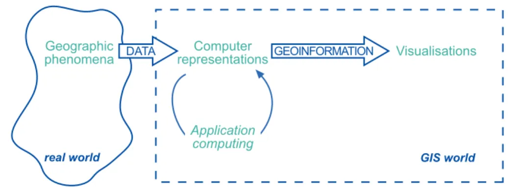
Principles of Geographic Information Systems (GIS): an Introductory Textbook - Free Computer, Programming, Mathematics, Technical Books, Lecture Notes and Tutorials

Full text

(1)Principles of Geographic Information Systems An introductory textbook. Editors Otto Huisman and Rolf A. de By. previous. next. back. exit. contents. index. glossary. web links. bibliography. about.

(2) Cover illustration: Paul Klee (1879–1940), Chosen Site (1927) Pen-drawing and water-colour on paper. Original size: 57.8 × 40.5 cm. Private collection, Munich c Paul Klee, Chosen Site, 2001 c/o Beeldrecht Amstelveen Cover page design: Wim Feringa All rights reserved. No part of this book may be reproduced or translated in any form, by print, photoprint, microfilm, microfiche or any other means without written permission from the publisher. Published by: The International Institute for Geo-Information Science and Earth Observation (ITC), Hengelosestraat 99, P.O. Box 6, 7500 AA Enschede, The Netherlands CIP-GEGEVENS KONINKLIJKE BIBLIOTHEEK, DEN HAAG. Principles of Geographic Information Systems Otto Huisman, Rolf A. de By (eds.) (ITC Educational Textbook Series; 1) previous. next. back. exit. contents. index. glossary. web links. bibliography. about.

(3) Fourth edition ISBN 978–90–6164–269–5 ITC, Enschede, The Netherlands ISSN 1567–5777 ITC Educational Textbook Series c 2009 by ITC, Enschede, The Netherlands.

(4) Contents 1. 2. A gentle introduction to GIS 1.1 The nature of GIS . . . . . . . . . . . . . . . . . . . 1.1.1 Some fundamental observations . . . . . . 1.1.2 Defining GIS . . . . . . . . . . . . . . . . . . 1.1.3 GISystems, GIScience and GIS applications 1.1.4 Spatial data and geoinformation . . . . . . 1.2 The real world and representations of it . . . . . . 1.2.1 Models and modelling . . . . . . . . . . . . 1.2.2 Maps . . . . . . . . . . . . . . . . . . . . . . 1.2.3 Databases . . . . . . . . . . . . . . . . . . . 1.2.4 Spatial databases and spatial analysis . . . 1.3 Structure of this book . . . . . . . . . . . . . . . . .. . . . . . . . . . . .. 25 26 29 32 43 45 48 49 51 53 55 57. Geographic information and Spatial data types 2.1 Models and representations of the real world . . . . . . . . . . . . 2.2 Geographic phenomena . . . . . . . . . . . . . . . . . . . . . . . . 2.2.1 Defining geographic phenomena . . . . . . . . . . . . . . .. 62 63 66 67. previous. next. back. exit. contents. index. . . . . . . . . . . .. glossary. . . . . . . . . . . .. . . . . . . . . . . .. . . . . . . . . . . .. . . . . . . . . . . .. . . . . . . . . . . .. . . . . . . . . . . .. web links. . . . . . . . . . . .. bibliography. about. 4.

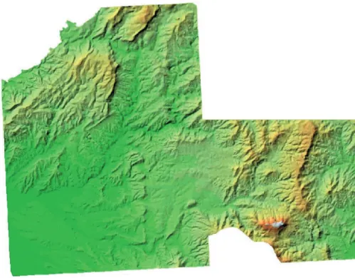
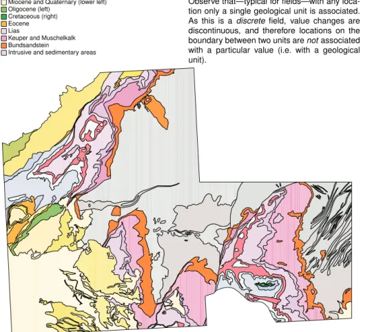
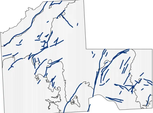
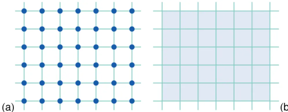
(5) 2.3. 2.4 2.5 3. 2.2.2 Types of geographic phenomena . . . . . . . . 2.2.3 Geographic fields . . . . . . . . . . . . . . . . . 2.2.4 Geographic objects . . . . . . . . . . . . . . . . 2.2.5 Boundaries . . . . . . . . . . . . . . . . . . . . Computer representations of geographic information 2.3.1 Regular tessellations . . . . . . . . . . . . . . . 2.3.2 Irregular tessellations . . . . . . . . . . . . . . 2.3.3 Vector representations . . . . . . . . . . . . . . 2.3.4 Topology and spatial relationships . . . . . . . 2.3.5 Scale and resolution . . . . . . . . . . . . . . . 2.3.6 Representations of geographic fields . . . . . . 2.3.7 Representation of geographic objects . . . . . . Organizing and managing spatial data . . . . . . . . . The temporal dimension . . . . . . . . . . . . . . . . .. Data management and processing systems 3.1 Hardware and software trends . . . . . . . . 3.2 Geographic information systems . . . . . . . 3.2.1 GIS software . . . . . . . . . . . . . . . 3.2.2 GIS architecture and functionality . . 3.2.3 Spatial Data Infrastructure (SDI) . . . 3.3 Stages of spatial data handling . . . . . . . . 3.3.1 Spatial data capture and preparation . 3.3.2 Spatial data storage and maintenance 3.3.3 Spatial query and analysis . . . . . . . 3.3.4 Spatial data presentation . . . . . . . . 3.4 Database management systems . . . . . . . .. . . . . . . . . . . .. . . . . . . . . . . .. . . . . . . . . . . .. . . . . . . . . . . .. . . . . . . . . . . .. . . . . . . . . . . . . . . . . . . . . . . . . .. . . . . . . . . . . . . . . . . . . . . . . . . .. . . . . . . . . . . . . . . . . . . . . . . . . .. . . . . . . . . . . . . . . . . . . . . . . . . .. . . . . . . . . . . . . . . . . . . . . . . . . .. . . . . . . . . . . . . . . . . . . . . . . . . .. . . . . . . . . . . . . . .. 69 72 77 81 82 85 88 91 101 113 114 119 124 126. . . . . . . . . . . .. 135 137 140 142 144 146 148 149 151 155 157 158.

(6) 3.5. 4. 5. 3.4.1 Reasons for using a DBMS . . . . . 3.4.2 Alternatives for data management 3.4.3 The relational data model . . . . . 3.4.4 Querying a relational database . . GIS and spatial databases . . . . . . . . . 3.5.1 Linking GIS and DBMS . . . . . . 3.5.2 Spatial database functionality . . .. . . . . . . .. . . . . . . .. . . . . . . .. . . . . . . .. . . . . . . .. . . . . . . .. . . . . . . .. . . . . . . .. . . . . . . .. . . . . . . .. . . . . . . .. . . . . . . .. . . . . . . .. . . . . . . .. 160 163 164 171 178 179 182. Spatial referencing and positioning 4.1 Spatial referencing . . . . . . . . . . . . . 4.1.1 Reference surfaces for mapping . . 4.1.2 Coordinate systems . . . . . . . . . 4.1.3 Map projections . . . . . . . . . . . 4.1.4 Coordinate transformations . . . . 4.2 Satellite-based positioning . . . . . . . . . 4.2.1 Absolute positioning . . . . . . . . 4.2.2 Errors in absolute positioning . . . 4.2.3 Relative positioning . . . . . . . . 4.2.4 Network positioning . . . . . . . . 4.2.5 Code versus phase measurements 4.2.6 Positioning technology . . . . . . .. . . . . . . . . . . . .. . . . . . . . . . . . .. . . . . . . . . . . . .. . . . . . . . . . . . .. . . . . . . . . . . . .. . . . . . . . . . . . .. . . . . . . . . . . . .. . . . . . . . . . . . .. . . . . . . . . . . . .. . . . . . . . . . . . .. . . . . . . . . . . . .. . . . . . . . . . . . .. . . . . . . . . . . . .. . . . . . . . . . . . .. 189 191 192 206 217 227 236 238 246 254 256 257 258. Data entry and preparation 5.1 Spatial data input . . . . . . . . . . . . . 5.1.1 Direct spatial data capture . . . . 5.1.2 Indirect spatial data capture . . . 5.1.3 Obtaining spatial data elsewhere. . . . .. . . . .. . . . .. . . . .. . . . .. . . . .. . . . .. . . . .. . . . .. . . . .. . . . .. . . . .. . . . .. . . . .. 270 271 272 274 280. . . . ..

(7) 5.2. 5.3. 5.4. 6. Data quality . . . . . . . . . . . . . . . . . . . . 5.2.1 Accuracy and precision . . . . . . . . . 5.2.2 Positional accuracy . . . . . . . . . . . . 5.2.3 Attribute accuracy . . . . . . . . . . . . 5.2.4 Temporal accuracy . . . . . . . . . . . . 5.2.5 Lineage . . . . . . . . . . . . . . . . . . . 5.2.6 Completeness . . . . . . . . . . . . . . . 5.2.7 Logical consistency . . . . . . . . . . . . Data preparation . . . . . . . . . . . . . . . . . 5.3.1 Data checks and repairs . . . . . . . . . 5.3.2 Combining data from multiple sources Point data transformation . . . . . . . . . . . . 5.4.1 Interpolating discrete data . . . . . . . . 5.4.2 Interpolating continuous data . . . . . .. Spatial data analysis 6.1 Classification of analytical GIS capabilities 6.2 Retrieval, classification and measurement . 6.2.1 Measurement . . . . . . . . . . . . . 6.2.2 Spatial selection queries . . . . . . . 6.2.3 Classification . . . . . . . . . . . . . 6.3 Overlay functions . . . . . . . . . . . . . . . 6.3.1 Vector overlay operators . . . . . . . 6.3.2 Raster overlay operators . . . . . . . 6.3.3 Overlays using a decision table . . . 6.4 Neighbourhood functions . . . . . . . . . . 6.4.1 Proximity computations . . . . . . .. . . . . . . . . . . .. . . . . . . . . . . .. . . . . . . . . . . . . . . . . . . . . . . . . .. . . . . . . . . . . . . . . . . . . . . . . . . .. . . . . . . . . . . . . . . . . . . . . . . . . .. . . . . . . . . . . . . . . . . . . . . . . . . .. . . . . . . . . . . . . . . . . . . . . . . . . .. . . . . . . . . . . . . . . . . . . . . . . . . .. . . . . . . . . . . . . . . . . . . . . . . . . .. . . . . . . . . . . . . . . . . . . . . . . . . .. . . . . . . . . . . . . . . . . . . . . . . . . .. . . . . . . . . . . . . . . . . . . . . . . . . .. . . . . . . . . . . . . . .. 284 285 287 298 300 301 302 303 304 305 312 320 323 325. . . . . . . . . . . .. 342 344 349 350 355 368 376 377 381 390 392 395.

(8) 6.5 6.6 6.7. 7. 6.4.2 Computation of diffusion . . . . . . . 6.4.3 Flow computation . . . . . . . . . . . 6.4.4 Raster based surface analysis . . . . . Network analysis . . . . . . . . . . . . . . . . GIS and application models . . . . . . . . . . Error propagation in spatial data processing 6.7.1 How errors propagate . . . . . . . . . 6.7.2 Quantifying error propagation . . . .. Data visualization 7.1 GIS and maps . . . . . . . . . . . . . . . . . 7.2 The visualization process . . . . . . . . . . . 7.3 Visualization strategies: present or explore? 7.4 The cartographic toolbox . . . . . . . . . . . 7.4.1 What kind of data do I have? . . . . 7.4.2 How can I map my data? . . . . . . 7.5 How to map . . . ? . . . . . . . . . . . . . . . 7.5.1 How to map qualitative data . . . . 7.5.2 How to map quantitative data . . . 7.5.3 How to map the terrain elevation . . 7.5.4 How to map time series . . . . . . . 7.6 Map cosmetics . . . . . . . . . . . . . . . . . 7.7 Map dissemination . . . . . . . . . . . . . .. . . . . . . . . . . . . .. . . . . . . . .. . . . . . . . .. . . . . . . . .. . . . . . . . .. . . . . . . . .. . . . . . . . .. . . . . . . . .. . . . . . . . .. . . . . . . . .. . . . . . . . .. . . . . . . . .. . . . . . . . .. 400 403 405 415 424 429 430 434. . . . . . . . . . . . . .. . . . . . . . . . . . . .. . . . . . . . . . . . . .. . . . . . . . . . . . . .. . . . . . . . . . . . . .. . . . . . . . . . . . . .. . . . . . . . . . . . . .. . . . . . . . . . . . . .. . . . . . . . . . . . . .. . . . . . . . . . . . . .. . . . . . . . . . . . . .. . . . . . . . . . . . . .. 440 441 452 456 463 464 466 470 471 473 477 481 485 490. Glossary. 504. A Internet sites. 536.

(9) List of Figures 1.1 1.2 1.3 1.4. The El Niño event of 1997 compared with a normal year 1998 . Schema of an SST measuring buoy . . . . . . . . . . . . . . . . The array of measuring buoys . . . . . . . . . . . . . . . . . . . Just four measuring buoys . . . . . . . . . . . . . . . . . . . . .. . . . .. 2.1 2.2 2.3 2.4 2.5 2.6 2.7 2.8 2.9 2.10 2.11 2.12. Three views of objects of study in GIS . . . . Elevation as a geographic field . . . . . . . . Geological units as a discrete field . . . . . . Geological faults as geographic objects . . . . Three regular tessellation types . . . . . . . . A grid and a raster illustrated . . . . . . . . . An example region quadtree . . . . . . . . . . Input data for a TIN construction . . . . . . . Two triangulations from the same input data An example line representation . . . . . . . . An example area representation . . . . . . . . Polygons in a boundary model . . . . . . . .. . 64 . 71 . 74 . 79 . 85 . 86 . 89 . 92 . 93 . 97 . 98 . 100. previous. next. back. exit. contents. index. . . . . . . . . . . . .. . . . . . . . . . . . .. . . . . . . . . . . . .. glossary. . . . . . . . . . . . .. . . . . . . . . . . . .. . . . . . . . . . . . .. . . . . . . . . . . . .. . . . . . . . . . . . .. . . . . . . . . . . . .. web links. . . . . . . . . . . . .. 30 35 36 60. bibliography. about. 9.

(10) 2.13 2.14 2.15 2.16 2.17 2.18 2.19 2.20 2.21 2.22 2.23 2.24 2.25. Example topological transformation . . . . . . . . . Simplices and a simplicial complex . . . . . . . . . . Spatial relationships between two regions . . . . . . The five rules of topological consistency in 2D space Raster representation of a continuous field . . . . . . Vector representation of a continuous field . . . . . . Image classification of an agricultural area . . . . . . Image classification of an urban area . . . . . . . . . A straight line and its raster representation . . . . . Geographic objects and their vector representation . Overlaying different rasters . . . . . . . . . . . . . . Producing a raster overlay layer . . . . . . . . . . . . Change detection from radar imagery . . . . . . . .. . . . . . . . . . . . . .. . . . . . . . . . . . . .. . . . . . . . . . . . . .. . . . . . . . . . . . . .. . . . . . . . . . . . . .. . . . . . . . . . . . . .. . . . . . . . . . . . . .. 102 105 108 110 115 117 120 121 122 123 124 125 130. 3.1 3.2 3.3 3.4 3.5 3.6 3.7 3.8 3.9. Functional components of a GIS . . . . . . Example relational database . . . . . . . . Example foreign key attribute . . . . . . . The two unary query operators . . . . . . The binary query operator . . . . . . . . . A combined query . . . . . . . . . . . . . Raster data and associated database table Vector data and associated database table Geometry data stored in spatial database. . . . . . . . . .. . . . . . . . . .. . . . . . . . . .. . . . . . . . . .. . . . . . . . . .. . . . . . . . . .. . . . . . . . . .. . . . . . . . . .. 145 165 170 175 176 177 180 181 183. 4.1 4.2 4.3 4.4. Two reference surfaces for approximating the Earth The Geoid . . . . . . . . . . . . . . . . . . . . . . . . Levelling network . . . . . . . . . . . . . . . . . . . . An oblate ellipse . . . . . . . . . . . . . . . . . . . . .. . . . .. . . . .. . . . .. . . . .. . . . .. . . . .. . . . .. 192 193 195 196. . . . . . . . . .. . . . . . . . . .. . . . . . . . . .. . . . . . . . . .. . . . . . . . . ..

(11) 4.5 4.6 4.7 4.8 4.9 4.10 4.11 4.12 4.13 4.14 4.15 4.16 4.17 4.18 4.19 4.20 4.21 4.22 4.23 4.24 4.25 4.26 4.27 4.28. Regionally best fitting ellipsoid . . . . . . . . . . . . . . . . . Dutch triangulation network . . . . . . . . . . . . . . . . . . . The ITRS and ITRF . . . . . . . . . . . . . . . . . . . . . . . . Height above the geocentric ellipsoid and above the Geoid . 2D geographic coordinate system . . . . . . . . . . . . . . . . 3D geographic coordinate system . . . . . . . . . . . . . . . . 3D geocentric coordinate system . . . . . . . . . . . . . . . . 2D cartesian coordinate system . . . . . . . . . . . . . . . . . Coordinate system of the Netherlands . . . . . . . . . . . . . 2D polar coordinate system . . . . . . . . . . . . . . . . . . . Projecting geographic into cartesian coordinates . . . . . . . Classes of map projections . . . . . . . . . . . . . . . . . . . . Three secant projection classes . . . . . . . . . . . . . . . . . . A transverse and an oblique projection . . . . . . . . . . . . . Mercator projection . . . . . . . . . . . . . . . . . . . . . . . . Cylindrical equal-area projection . . . . . . . . . . . . . . . . Equidistant cylindrical projection . . . . . . . . . . . . . . . . Changing map projection . . . . . . . . . . . . . . . . . . . . Changing projection combined with a datum transformation Determining pseudorange and position . . . . . . . . . . . . Satellite positioning . . . . . . . . . . . . . . . . . . . . . . . . Positioning satellites in view . . . . . . . . . . . . . . . . . . . Geometric dilution of precision . . . . . . . . . . . . . . . . . GPS satellite constellation . . . . . . . . . . . . . . . . . . . .. . . . . . . . . . . . . . . . . . . . . . . . .. . . . . . . . . . . . . . . . . . . . . . . . .. 198 201 202 205 207 209 211 212 214 215 218 221 221 222 224 225 226 230 232 239 242 250 253 260. 5.1 5.2. The phases of the vectorization process . . . . . . . . . . . . . . 278 Good/bad accuracy against good/bad precision . . . . . . . . . 286.

(12) 5.3 5.4 5.5 5.6 5.7 5.8 5.9 5.10 5.11 5.12 5.13 5.14 5.15 5.16 5.17 5.18. The positional error of a measurement . . . . . . . . . . . . A normally distributed random variable . . . . . . . . . . . Normal bivariate distribution . . . . . . . . . . . . . . . . . The ε- or Perkal band . . . . . . . . . . . . . . . . . . . . . . Point-in-polygon test with the ε-band . . . . . . . . . . . . Crisp and uncertain membership functions . . . . . . . . . Successive clean-up operations for vector data . . . . . . . The integration of two vector data sets may lead to slivers Multi-scale and multi-representation systems compared . . Multiple adjacent data sets can be matched and merged . . Interpolating quantitative and qualitative measurements . Generation of Thiessen polygons for qualitative data . . . . Various global trend surfaces . . . . . . . . . . . . . . . . . Interpolation by triangulation . . . . . . . . . . . . . . . . . The principle of moving window averaging . . . . . . . . . Inverse distance weighting as an averaging technique . . .. . . . . . . . . . . . . . . . .. . . . . . . . . . . . . . . . .. . . . . . . . . . . . . . . . .. 289 291 292 294 294 297 307 313 316 317 321 324 327 331 332 334. 6.1 6.2 6.3 6.4 6.5 6.6 6.7 6.8 6.9 6.10. Minimal bounding boxes . . . . . . . . . . . . . . . . . . . . Interactive feature selection . . . . . . . . . . . . . . . . . . Spatial selection through attribute conditions . . . . . . . . Further spatial selection through attribute conditions . . . Spatial selection using containment . . . . . . . . . . . . . . Spatial selection using intersection . . . . . . . . . . . . . . Spatial selection using adjacency . . . . . . . . . . . . . . . Spatial selection using the distance function . . . . . . . . . Two classifications of average household income per ward Example discrete classification . . . . . . . . . . . . . . . . .. . . . . . . . . . .. . . . . . . . . . .. . . . . . . . . . .. 352 357 358 359 363 364 365 366 369 372.

(13) 6.11 6.12 6.13 6.14 6.15 6.16 6.17 6.18 6.19 6.20 6.21 6.22 6.23 6.24 6.25 6.26 6.27 6.28 6.29 6.30 6.31. Two automatic classification techniques . . . . . . . . . . . . . The polygon intersect overlay operator . . . . . . . . . . . . . . The residential areas of Ilala District . . . . . . . . . . . . . . . Two more polygon overlay operators . . . . . . . . . . . . . . . Examples of arithmetic map algebra expressions . . . . . . . . Logical expressions in map algebra . . . . . . . . . . . . . . . . Complex logical expressions in map algebra . . . . . . . . . . . Examples of conditional raster expressions . . . . . . . . . . . The use of a decision table in raster overlay . . . . . . . . . . . Buffer zone generation . . . . . . . . . . . . . . . . . . . . . . . Thiessen polygon construction from a Delaunay triangulation Diffusion computations on a raster . . . . . . . . . . . . . . . . Flow computations on a raster . . . . . . . . . . . . . . . . . . . Moving window rasters for filtering . . . . . . . . . . . . . . . Slope angle defined . . . . . . . . . . . . . . . . . . . . . . . . . Slope angle and slope aspect defined . . . . . . . . . . . . . . . Part of a network with associated turning costs at a node . . . Ordered and unordered optimal path finding . . . . . . . . . . Network allocation on a pupil/school assignment problem . . Tracing functions on a network . . . . . . . . . . . . . . . . . . Error propagation in spatial data handling . . . . . . . . . . . .. . . . . . . . . . . . . . . . . . . . . .. 375 377 378 380 383 386 387 389 391 396 399 401 404 410 411 413 417 419 421 422 430. 7.1 7.2 7.3 7.4 7.5. Maps and location . . . . . . . . . . . . . Maps and characteristics . . . . . . . . . Maps and time . . . . . . . . . . . . . . . Comparing aerial photograph and map Topographic map of Overijssel . . . . .. . . . . .. 442 443 444 445 449. . . . . .. . . . . .. . . . . .. . . . . .. . . . . .. . . . . .. . . . . .. . . . . .. . . . . .. . . . . .. . . . . .. . . . . .. . . . . ..

(14) 7.6 7.7 7.8 7.9 7.10 7.11 7.12 7.13 7.14 7.15 7.16 7.17 7.18 7.19 7.20 7.21 7.22 7.23 7.24. Thematic maps . . . . . . . . . . . . . . . Dimensions of spatial data . . . . . . . . . Cartographic visualization process . . . . Visual thinking and communication . . . The cartographic communication process Bertin’s six visual variables . . . . . . . . Qualitative data map . . . . . . . . . . . . Two wrongly designed qualitative maps . Mapping absolute quantitative data . . . Two wrongly designed quantitative maps Mapping relative quantitative data . . . . Bad relative quantitative data maps . . . . Visualization of the terrain . . . . . . . . . Quantitative data in 3D visualization . . . Mapping change . . . . . . . . . . . . . . . The map and its information . . . . . . . . Text in the map . . . . . . . . . . . . . . . Visual hierarchy . . . . . . . . . . . . . . . Classification of maps on the WWW . . .. . . . . . . . . . . . . . . . . . . .. . . . . . . . . . . . . . . . . . . .. . . . . . . . . . . . . . . . . . . .. . . . . . . . . . . . . . . . . . . .. . . . . . . . . . . . . . . . . . . .. . . . . . . . . . . . . . . . . . . .. . . . . . . . . . . . . . . . . . . .. . . . . . . . . . . . . . . . . . . .. . . . . . . . . . . . . . . . . . . .. . . . . . . . . . . . . . . . . . . .. . . . . . . . . . . . . . . . . . . .. . . . . . . . . . . . . . . . . . . .. . . . . . . . . . . . . . . . . . . .. 450 451 452 458 461 467 471 472 473 474 475 476 479 480 484 487 488 489 491.

(15) List of Tables 1.1 1.2. Average sea surface temperatures in December 1997 . . . . . . . . Database table of daily buoy measurements . . . . . . . . . . . . .. 3.1 3.2 3.3 3.4 3.5. Commonly used unit prefixes . . . . . . . . . Spatial data input methods and devices used Raster and vector representations compared Spatial data presentation . . . . . . . . . . . . Three relation schemas . . . . . . . . . . . . .. . . . . .. . . . . .. . . . . .. . . . . .. . . . . .. 138 150 152 157 167. 4.1 4.2 4.3 4.4. Three global ellipsoids . . . . . . . . . . . . . . . . . . . . . Transformation of Cartesian coordinates . . . . . . . . . . . Transformation from the Potsdam datum . . . . . . . . . . Magnitude of errors in absolute satellite-based positioning. . . . .. . . . .. . . . .. . . . .. 199 234 235 252. 5.1 5.2. A simple error matrix . . . . . . . . . . . . . . . . . . . . . . . . . . 299 Clean-up operations for vector data . . . . . . . . . . . . . . . . . 306. 6.1. Example continuous classification table . . . . . . . . . . . . . . . 370. previous. next. back. exit. contents. index. . . . . .. . . . . .. . . . . .. . . . . .. glossary. . . . . .. . . . . .. . . . . .. web links. 40 54. bibliography. about. 15.

(16) 6.2. Common causes of error in spatial data handling . . . . . . . . . . 433. 7.1 7.2. Data nature and measurement scales . . . . . . . . . . . . . . . . . 465 Measurement scales linked to visual variables . . . . . . . . . . . 469.

(17) Preface This book was originally designed for a three-week lecturing module on the principles of Geographic Information Systems (GIS), to be taught to students in all education programmes at ITC as the second module in their course. A geographic information system is a computer-based system that supports the study of natural and man-made phenomena with an explicit location in space. To this end, the GIS allows data entry, data manipulation, and production of interpretable output that may provide new insights about the phenomena. There are many uses for GIS technology, including soil science; management of agricultural, forest and water resources; urban planning; geology; mineral exploration; cadastre and environmental monitoring. It is likely that the student reader of this textbook is already educated in one of these fields; the intention of the book is to lay the foundation for the reader to also become proficient in the use of GIS technology. With so many different fields of application, it is impossible to single out the specific techniques of GIS usage for all the fields in a single book. Rather, the. previous. next. back. exit. contents. index. glossary. web links. bibliography. about. 17.

(18) 18. Preface book focuses on a number of common and important topics that any expert GIS user should be aware of. GIS is a continuously evolving scientific discipline, and for this reason ITC students should be provided with a broad foundation of relevant concepts, techniques and technology. The book is also meant to define a common understanding and terminology for follow-up modules, which the student may elect later in her/his respective programme. The textbook does not stand independently, but was developed in conjunction with the textbook on Principles of Remote Sensing.. previous. next. back. exit. contents. index. glossary. web links. bibliography. about.

(19) 19. Preface. Structure of this book The chapters of the book have been arranged in a semi-classical set-up. Chapters 1 to 3 provide a general introduction to the field, discussing various interesting geographic phenomena (Chapter 1), the ways these phenomena can be represented in a computer system (Chapter 2), and the data processing systems that are used to this end (Chapter 3). Spatial referencing and positioning (including map projections and GPS) is dealt with in Chapter 4. Chapters 5 to 7 subsequently focus on the process of using a GIS environment. We discuss how spatial data can be obtained, entered and prepared for use (Chapter 5), how data can be manipulated to improve our understanding of the phenomena that they represent (Chapter 6), and how the results of such manipulations can be visualized (Chapter 7). Special attention throughout these chapters is devoted to the specific characteristics of geospatial data. Each chapter contains sections, a summary and some exercises. The exercises are meant to be a test of understanding of the chapter’s contents; they are not practical exercises. They may not be typical exam questions either! Besides the regular chapters, the back part of the book contains a bibliography, a glossary, and an index. The book is also made available as an electronic PDF document which can be browsed but not printed.. previous. next. back. exit. contents. index. glossary. web links. bibliography. about.

(20) 20. Preface. Acknowledgements The book has a significant history, dating from the 1999 curriculum. This is a heavily revised, in parts completely rewritten, version of that first edition. Major contributors to the current content of this book include Rolf de By, Richard Knippers, Michael Weir, Yola Georgiadou, Menno-Jan Kraak, Cees van Westen and Yuxian Sun. Authors of the original text include Martin Ellis, Wolfgang Kainz, Mostafa Radwan and Ed Sides. Other contributors which deserve a great deal of credit for their management, assistance and/or advisory roles in the production of previous editions of this book include Erica Weijer, Marion van Rinsum, Ineke ten Dam, Kees Bronsveld, Rob Lemmens, Connie Blok, Allan Brown, Corné van Elzakker, Lucas Janssen, Barend Köbben, Bart Krol, and Jan Hendrikse. Facilitated by technical advice from Wim Feringa, many illustrations in the book were produced from data sources provided by Sherif Amer, Wietske Bijker, Wim Feringa, Robert Hack, Asli Harmanli, Gerard Reinink, Richard Sliuzas, Siefko Slob, and Yuxian Sun. In some cases, because of the data’s history, they can perhaps be better ascribed to an ITC division: Cartography, Engineering Geology, and Urban Planning and Management. For this fourth edition, a number of colleagues provided valuable comments and prepared materials that helped to substantially improve the existing text. They include Richard Knippers, Connie Blok, Ellen-Wien Augustijn, Rob Lemmens, Wim Bakker, Ivana Ivanova, Nicholas Hamm, Jelger Kooistra, Chris Hecker and Karl Grabmaier. Wim Feringa deserves special thanks for providing new and. previous. next. back. exit. contents. index. glossary. web links. bibliography. about.

(21) 21. Preface redrawn figures for this edition, as well as his work on the updated cover design. The editors would also like to acknowledge the pleasant collaboration with Klaus Tempfli, the editor of Principles of Remote Sensing and Coco Rulinda for LATEX issues.. previous. next. back. exit. contents. index. glossary. web links. bibliography. about.

(22) 22. Preface. Technical account This book was written using Leslie Lamport’s LATEX generic typesetting system, which uses Donald Knuth’s TEX as its formatting engine. Figures came from various sources, but many were eventually prepared with Macromedia’s Freehand package, and then turned into PDF format. From the LATEX sources we generated the book in PDF format, using the PDFLATEX macro package, supported by various add-on packages, the most important being Sebastian Rahtz’ hyperref.. previous. next. back. exit. contents. index. glossary. web links. bibliography. about.

(23) 23. Preface. Preface to the fourth edition This fourth edition of the GIS book is an update of the previous edition, with some reshuffling of the book’s content and some minor changes to the layout (marginal editorial disagreements notwithstanding). Care has been taken to provide updated material, improve readability and browse-ability of the text, and achieve greater integration through cross-referencing. Significant changes include a rewritten section on spatial referencing by Richard Knippers, restructuring of material in chapters 3, 4 and 5, and a range of edits for improved continuity throughout the chapters. A keyword–in–the–margin layout was adopted to aid in browse-ability of the main text. It must be stressed that the design of this book remains that of a textbook on ‘principles’. A much bigger overhaul would have been required for another format, and this was considered undesirable for its purpose, and infeasible in the time allowed, also because of dependencies with already developed teaching materials such as exercises and overhead slides. This textbook continues to be used at ITC in all educational programmes, as well as in other programmes around the globe that are developed in collaboration with ITC. A Korean translation of both textbooks has already been published, and other translation projects are under way. People with an interest in such an undertaking are invited to contact the editors. A book such as this will never be perfect, and the field of GIScience has not yet reached the type of maturity where debates over definitions and descriptions are no longer needed. The Editors welcome any comments and criticisms, in a. previous. next. back. exit. contents. index. glossary. web links. bibliography. about.

(24) 24. Preface continued effort to improve the materials.. Otto Huisman and Rolf A. de By, Enschede, July 2009. previous. next. back. exit. contents. index. glossary. web links. bibliography. about.

(25) Chapter 1 A gentle introduction to GIS. previous. next. back. exit. contents. index. glossary. web links. bibliography. about. 25.

(26) 26. 1.1. The nature of GIS. 1.1. The nature of GIS. The purpose of this chapter is to set the scene for the remainder of this book by providing a general overview of some of the terms, concepts and ideas which will be covered in greater detail in later sections. The acronym GIS stands for geographic information system. As the name suggests, a GIS is a tool for working with geographic information. Section 1.1.2 provides a more formal definition, and later sections will look in more detail at some of the key functions that set GIS apart from other kinds of information systems. GIS have rapidly developed since the late 1970’s in terms of both technical and processing capabilities, and today are widely used all over the world for a wide range of purposes. Let us begin by looking at some of these:. Geographic information system. • An urban planner might want to assess the extent of urban fringe growth in her/his city, and quantify the population growth that some suburbs are witnessing. S/he might also like to understand why these particular suburbs are growing and others are not; • A biologist might be interested in the impact of slash-and-burn practices on the populations of amphibian species in the forests of a mountain range to obtain a better understanding of long-term threats to those populations; • A natural hazard analyst might like to identify the high-risk areas of annual monsoon-related flooding by investigating rainfall patterns and terrain characteristics;. previous. next. back. exit. contents. index. glossary. web links. bibliography. about.

(27) 27. 1.1. The nature of GIS • A geological engineer might want to identify the best localities for constructing buildings in an earthquake-prone area by looking at rock formation characteristics; • A mining engineer could be interested in determining which prospective copper mines should be selected for future exploration, taking into account parameters such as extent, depth and quality of the ore body, amongst others; • A geoinformatics engineer hired by a telecommunications company may want to determine the best sites for the company’s relay stations, taking into account various cost factors such as land prices, undulation of the terrain et cetera; • A forest manager might want to optimize timber production using data on soil and current tree stand distributions, in the presence of a number of operational constraints, such as the need to preserve species diversity in the area; • A hydrological engineer might want to study a number of water quality parameters of different sites in a freshwater lake to improve understanding of the current distribution of Typha reed beds, and why it differs from that of a decade ago. In the examples presented above, all the professionals work with positional data – also called spatial data. Spatial data refers to where things are, or perhaps, where they were or will be. To be more precise, these professionals deal with questions related to geographic space,which we define as having positional data relative to the Earth’s surface. previous. next. back. exit. contents. index. glossary. web links. bibliography. Spatial data. about.

(28) 28. 1.1. The nature of GIS Positional data of a non-geographic nature also exists. Examples include the location of the appendix in the human body, or the location of headlights on a car. these examples involve positional information, but it makes no sense to use the Earth’s surface as a reference for these applications. For the purposes of this book we are only interested in geographic data. To illustrate these issues further, the following section provides an example of the application of GIS to the study of global weather patterns.. previous. next. back. exit. contents. index. glossary. web links. bibliography. Geographic data. about.

(29) 29. 1.1. The nature of GIS. 1.1.1. Some fundamental observations. Our world is dynamic. Many aspects of our daily lives and our environment are constantly changing, and not always for the better. Some of these changes appear to have natural causes (e.g. volcanic eruptions, meteorite impacts), while others are the result of human modification of the environment (e.g. land use changes or land reclamation from the sea, a favourite pastime of the Dutch). There are also a large number of global changes for which the cause remains unclear: these include global warming, the El Niño/La Niña events, or at smaller scales, landslides and soil erosion. In summary, we can say that changes to the Earth’s geography can have natural or man-made causes, or a mix of both. If it is a mix of causes, we usually do not fully understand the changes.. Dynamics and change. For background information on El Niño, please refer to Figure 1.1. This Figure presents information related to a study area (the equatorial Pacific Ocean), with positional data taking a prominent role. Although quite a complex phenomenon, we will use the study of El Niño as an example application of GIS in the remainder of this chapter. In order to understand what is going on in our world, we study the processes or phenomena that bring about geographic change. In many cases, we want to broaden or deepen our understanding to help us make decisions, so that we can take the best course of action. For instance, if we understand El Niño better, and can forecast that another event may take place in the year 2012, we can devise an action plan to reduce the expected losses in the fishing industry, to lower the risks of landslides caused by heavy rains or to build up water supplies in areas of expected droughts.. previous. next. back. exit. contents. index. glossary. web links. Geographic phenomena. bibliography. about.

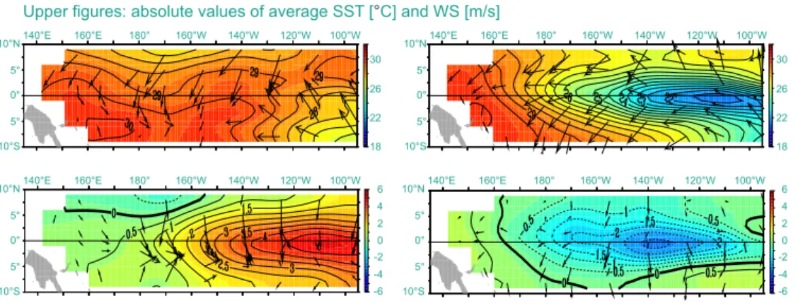
(30) 30. 1.1. The nature of GIS. El Niño is an aberrant pattern in weather and sea water temperature that occurs with some frequency (every 4–9 nine years) in the Pacific Ocean along the Equator. It is characterized by less strong western winds across the ocean, less upwelling of cold, nutrient-rich, deep-sea water near the South American coast, and therefore by substantially higher sea surface temperatures (see figures below). It is generally believed that El Niño has a considerable impact on global weather systems, and that it is the main cause for droughts in Wallacea and Australia, as well as for excessive rains in Peru and the southern U.S.A. El Niño means ‘little boy’, and manifests itself usually around Christmas. There exists also another—less pronounced–pattern of colder temperatures, that is known as La Niña (‘little girl’) which occurs less frequently than El Niño. The most recent occurrence of El Niño started in September 2006 and lasted until early 2007 From June 2007 on, data indicated a weak La Niña event, strengthening in early 2008. The figures below left illustrate an extreme El Niño year (1997; considered to be the most extreme of the twentieth century) and a subsequent La Niña year (1998). Left figures are from December 1997, an extreme El Niño event; right figures are of the subsequent year, indicating a La Niña event. In all figures, colour is used to indicate sea water temperature, while arrow lengths indicate wind speeds. The top figures provide information about absolute values, while the bottom figures are labelled with values relative to the average situation for the month of December. The bottom figures also give an indication of wind speed and direction. See also Figure 1.3 for an indication of the area covered by the array of buoys. December 1997 December 1998 Upper figures: absolute values of average SST [°C] and WS [m/s] 10°N. 140°E. 160°E. 180°. 160°W. 140°W. 120°W. 100°W. 10°N. 140°E. 160°E. 180°. 160°W. 140°W. 120°W. 100°W. 30 5°. 30 5°. 26. 0°. 26. 0°. 5°. 22. 5°. 22. 10°S. 18. 10°S. 18. 6. 10°N. 10°N. 140°E. 160°E. 180°. 160°W. 140°W. 120°W. 100°W. 4. 5°. 2. 0°. 0 -2. 5°. -4 -6. 10°S. 140°E. 160°E. 180°. 160°W. 140°W. 120°W. 100°W. 2. 0°. 0 -2. 5°. -4 -6. 10°S. Lower figures: differences with normal situation. previous. next. back. exit. contents. 6 4. 5°. index. glossary. web links. Figure 1.1: The El Niño event of 1997 compared with a more normal year 1998. The top figures indicate average Sea Surface Temperature (SST, in colour) and average Wind Speed (WS, in arrows) for the month of December. The bottom figures illustrate the anomalies (differences from a normal situation) in both SST and WS. The island in the lower left corner is (Papua) New Guinea with the Bismarck Archipelago. Latitude has been scaled by a factor two. Data source: National Oceanic and Atmospheric Administration, Pacific Marine Environmental Laboratory, Tropical Atmosphere Ocean project (NOAA/PMEL/TAO).. bibliography. about.

(31) 31. 1.1. The nature of GIS The fundamental problem that we face in many uses of GIS is that of understanding phenomena that have a spatial or geographic dimension, as well as a temporal dimension. We are facing ‘spatio-temporal’ problems. This means that our object of study has different characteristics for different locations (the geographic dimension) and also that these characteristics change over time (the temporal dimension). The El Niño event is a good example of such a phenomenon, because sea surface temperatures differ between locations, and sea surface temperatures change from one week to the next.. previous. next. back. exit. contents. index. glossary. web links. bibliography. Spatial and temporal dimensions. about.

(32) 32. 1.1. The nature of GIS. 1.1.2. Defining GIS. The previous section illustrated the use of GIS in a range of settings to operate on data that represent geographic phenomena. This provides us with a functional definition (after Aronoff [3]): A GIS is a computer-based system that provides the following four sets of capabilities to handle georeferenced data: 1. Data capture and preparation 2. Data management, including storage and maintenance 3. Data manipulation and analysis 4. Data presentation This implies that a GIS user can expect support from the system to enter (georeferenced) data, to analyse it in various ways, and to produce presentations (including maps and other types) from the data. This would include support for various kinds of coordinate systems and transformations between them, options for analysis of the georeferenced data, and obviously a large degree of freedom of choice in the way this information is presented (such as colour scheme, symbol set, and medium used). For examples of each of these capabilities, let us take a closer look at the El Niño example. Many professionals closely study this phenomenon, most notably meteorologists and oceanographers. They prepare all sorts of products, such as the. previous. next. back. exit. contents. index. glossary. web links. bibliography. about.

(33) 33. 1.1. The nature of GIS maps of Figure 1.1, in order to improve their understanding. To do so, they need to obtain data about the phenomenon, which, as shown above, includes measurements about sea water temperature and wind speed from many locations. This data must be stored and processed to enable it to be analysed, and allow the results from the analysis to be interpreted. The way this data is presented could play an important role in its interpretation. We have listed these capabilities above in the most natural order in which they take place. But this is only a sketch of an ideal situation, and it is often the case that data analysis suggests that we need more data about the problem. Data presentation may also lead to follow-up questions for which we need to do more analysis, and for which we may need more data, or perhaps better data. Consequently, several of the steps may be repeated a number of times before we are happy with the results. We look into these steps in more detail below, in the context of the El Niño example.. previous. next. back. exit. contents. index. glossary. web links. bibliography. about.

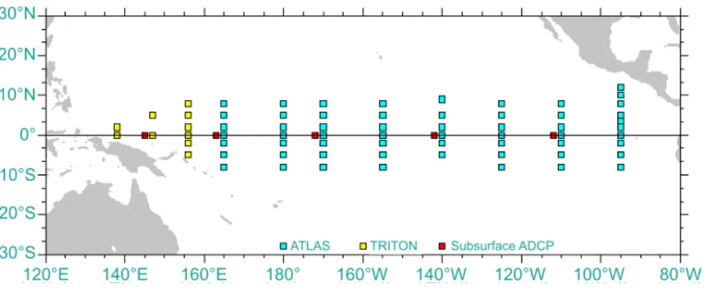
(34) 34. 1.1. The nature of GIS Data capture and preparation In the El Niño case, data capture refers to the collection of sea water temperatures and wind speed measurements. This is achieved by placing buoys with measuring equipment at various places in the ocean. Each buoy measures a number of things: wind speed and direction; air temperature and humidity; and sea water temperature at the surface and at various depths down to 500 metres. For the sake of our example we will focus on sea surface temperature (SST) and wind speed (WS). A typical buoy is illustrated in Figure 1.2, which shows the placement of various sensors on the buoy. For monitoring purposes, some 70 buoys were deployed at strategic places within 10◦ latitude of the Equator, between the Galápagos Islands and Papua New Guinea. Figure 1.3 provides a map that illustrates the positions of these buoys. The buoys have been anchored, so they are stationary. Occasional malfunctioning is caused by high seas and bad weather or by the buoys becoming entangled in long-line fishing nets.1 All the data that a buoy obtains through its thermometers and other sensors, as well as the buoy’s geographic position are transmitted by satellite communication daily. Later in this book, and also in the textbook on Principles of Remote Sensing [53], many other ways of acquiring geographic data will be discussed.. 1. As Figure 1.3 shows, there happen to be three types of buoy, but their differences are not directly relevant to our example, so we will ignore them here.. previous. next. back. exit. contents. index. glossary. web links. bibliography. about.

(35) 35. 1.1. The nature of GIS. Argos antenna 3.8 m above sea data logger. WS sensor humidity sensor Torroidal buoy Ø 2.3 m. SST sensor temperature sensors 3/8” wire rope. sensor cable. 500 m. temperature sensor. 3/4” nylon rope. Figure 1.2: Schematic overview of an ATLAS type buoy for monitoring sea water temperatures in the El Niño project. acoustic release NOAA. anchor 4200 lbs. previous. next. back. exit. contents. index. glossary. web links. bibliography. about.

(36) 36. 1.1. The nature of GIS. 30°N 20°N 10°N 0° 10°S 20°S 30°S 120°E. previous. next. ATLAS. 140°E. 160°E. back. exit. 180°. TRITON. 160°W. contents. Subsurface ADCP. 140°W. 120°W. 100°W. index. glossary. 80°W. web links. Figure 1.3: The array of positions of sea surface temperature and wind speed measuring buoys in the equatorial Pacific Ocean. bibliography. about.

(37) 37. 1.1. The nature of GIS Data management For our example application, data management refers to the storage and maintenance of the data transmitted by the buoys via satellite communication. This phase requires a decision to be made on how best to represent our data, both in terms of their spatial properties and the various attribute values which we need to store. Data storage and maintenance is discussed at length in Chapter 3, and we will not go into further detail here. We will from here on assume that the acquired data has been put in digital form, that is, it has been converted into computer-readable format, so that we can begin our analysis.. previous. next. back. exit. contents. index. glossary. web links. bibliography. about.

(38) 38. 1.1. The nature of GIS Data manipulation and analysis Once the data has been collected and organized in a computer system, we can start analysing it. Here, let us look at what processes were involved in the eventual production of the maps of Figure 1.1. Note that the actual production of maps belongs to the phase of data presentation that we discuss below. Here, we look at how data generated at the buoys was processed before map production. A closer look at Figure 1.1 reveals that the data being presented are based on the monthly averages for SST and WS (for two months), not on single measurements for a specific date. Moreover, the two lower figures provide comparisons with ‘the normal situation’, which probably means that a comparison was made with the December averages of several years. The initial (buoy) data have been generalized from 70 point measurements (one for each buoy) to cover the complete study area. Clearly, for positions in the study area for which no data was available, some type of interpolation took place, probably using data of nearby buoys. This is a typical GIS function: deriving an estimated value for a property for some location where we have not measured.. Sample measurements. It appears that the following steps took place for the upper two figures (here we look at SST computations only—WS analysis will have been similarly conducted): 1. For each buoy, the average SST for each month was computed, using the daily SST measurements for that month. This is a simple computation. 2. For each buoy, the monthly average SST was taken together with the geoprevious. next. back. exit. contents. index. glossary. web links. bibliography. about.

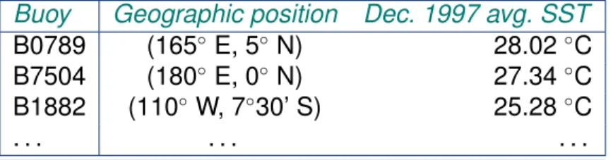
(39) 39. 1.1. The nature of GIS graphic location, to obtain a georeferenced list of averages, as illustrated in Table 1.1. 3. From this georeferenced list, through a method of spatial interpolation, the estimated SST of other positions in the study are were computed. This step was performed as often as needed, to obtain a fine mesh of positions with measured or estimated SSTs from which the maps of Figure 1.1 were eventually derived. 4. We assume that previous to the above steps we had obtained data about average SST for the month of December for a series of years. This too may have been spatially interpolated to obtain a ‘normal situation’ December data set of a fine resolution. Let us first clarify what is meant by a ‘georeferenced’ list. Data is georeferenced if it is associated with some position on the Earth’s surface, by using a spatial reference system. This can be achieved using (longitude, latitude) coordinates, or by other means that we discuss in Chapter 4. The key issue is that there is some kind of coordinate system as a reference. In our list, we have associated average sea surface temperature observations with spatial locations, and thereby we have georeferenced them. In step 3 above, we mentioned spatial interpolation. To understand this issue, it is important to note that sea surface temperature is a property that occurs everywhere in the ocean, and not only at the buoys where measurements are taken. The buoys only provide a set of sample observations of sea surface temperature.We can use these sample measurements to estimate the value of SST in places where we have not measured it, using a technique called spatial interpolation. The theory of spatial interpolation is extensive, but this is not the place to previous. next. back. exit. contents. index. glossary. web links. bibliography. Georeferenced data. Spatial interpolation. about.

(40) 40. 1.1. The nature of GIS Buoy B0789 B7504 B1882 .... Geographic position (165◦ E, 5◦ N) (180◦ E, 0◦ N) (110◦ W, 7◦ 30’ S) .... Table 1.1: The georeferenced list (in part) of average sea surface temperatures obtained for the month December 1997.. Dec. 1997 avg. SST 28.02 ◦ C 27.34 ◦ C 25.28 ◦ C .... discuss it. There are in fact many different spatial interpolation techniques, not just one, and some are better in specific situations than others. This is however a typical example of functions that a GIS can perform on user data.. previous. next. back. exit. contents. index. glossary. web links. bibliography. about.

(41) 41. 1.1. The nature of GIS Data presentation After the data manipulations discussed above, our data is prepared for producing output. In this case, the maps of Figure 1.1. The data presentation phase deals with putting it all together into a format that communicates the result of data analysis in the best possible way. Many issues arise in this phase. Among other things, we need to consider what the message is that we want to portray, who the audience is, what kind of presentation medium will be used, which rules of aesthetics apply, and what techniques are available for representation. These issues may sound a little abstract, so let us clarify with the El Niño case. For Figure 1.1, we can make the following statements: • The message we wanted to portray is what are the El Niño and La Niña events, both in absolute figures, but also in relative figures, i.e. as differences from a normal situation. • The audience for this data presentation clearly were the readers of this text book, i.e. students of ITC who want to obtain a better understanding of GIS. • The medium was this book, (printed matter of A4 size) and possibly a website. The book’s typesetting imposes certain restrictions, like maximum size, font style and font size. • The rules of aesthetics demanded many things: the maps should be printed north-up; with clear georeferencing; with intuitive use of symbols et cetera. previous. next. back. exit. contents. index. glossary. web links. bibliography. about.

(42) 42. 1.1. The nature of GIS We actually also violated some rules of aesthetics, for instance, by applying a different scaling factor in latitude (horizontally) compared to longitude (vertically). • The techniques that we used included the use of a colour scheme and isolines,2 plus a number of other techniques.. 2. Isolines are discussed in Chapter 2.. previous. next. back. exit. contents. index. glossary. web links. bibliography. about.

(43) 43. 1.1. The nature of GIS. 1.1.3. GISystems, GIScience and GIS applications. The previous discussion defined a geographic information system— in the ‘narrow’ sense—in terms of its functions as as a computerized system that facilitates the phases of data entry, data management, data analysis and data presentation specifically for dealing with georeferenced data. In the ‘wider’ sense, a functioning GIS requires both hardware and software, and also people such as the database creators or administrators, analysts who work with the software, and the users of the end product. For the purposes of this book we will concern ourselves with the ‘narrow’ definition, and focus on the specifics of these so-called GISystems.. GISystems. The discipline that deals with all aspects of the handling of spatial data and geoinformation is called geographic information science (often abbreviated to geoinformation science or just GIScience). Geo-Information Science is the scientific field that attempts to integrate different disciplines studying the methods and techniques of handling spatial information. Related terms include geoinformatics, geomatics, and spatial information science. These are all similar terms which have much the same meaning, although each approach has slight differences in the way it deals with problems, some emphasizing engineering approaches, others computational solutions, and so on.. GIScience. As well as being aware of these differences, it is also important to be aware of the difference between a geographic information system and and a GIS application. In the example discussed above (determining sea water temperatures of. previous. next. back. exit. contents. index. glossary. web links. bibliography. about.

(44) 44. 1.1. The nature of GIS the El Niño event in two subsequent December months). The same software package that we used to do this analysis could also be used to analyse forest plots in northern Thailand, for instance. That would be a different application, but would make use of the same software. GIS software can (generically) be applied to many different applications. When there is no risk of ambiguity, people sometimes do not make the distinction between a ‘GIS’ and a ‘GIS application’.. GIS applications. Project-based GIS applications usually have a clear-cut purpose, and these applications can be short-lived: the research is carried out by collecting data, entering data in the GIS, analysing the data, and producing informative maps. An example is rapid earthquake damage assessment. Institutional GIS applications, on the other hand, usually have as their goal the continued administration of spatial change and the sustained availability of spatial base data. Their needs for advanced data analysis are usually less, and the complexity of these applications lies more in the continued provision of trustworthy data to others. They are thus long-lived applications. An obvious example are automated cadastral systems.. previous. next. back. exit. contents. index. glossary. web links. bibliography. about.

(45) 45. 1.1. The nature of GIS. 1.1.4. Spatial data and geoinformation. A subtle difference exists between the terms data and information. Most of the time, we use the two terms almost interchangeably, and without the risk of confusing their meanings. Occasionally, however, we need to be precise about exactly what it is we are referring to, and in this situation their distinction does matter. By data, we mean representations that can be operated upon by a computer. More specifically, by spatial data we mean data that contains positional values, such as (x, y) co-ordinates. Sometimes the more precise phrase geospatial data is used as a further refinement, which refers to spatial data that is georeferenced. In this book, we will use ‘spatial data’ as a synonym for ‘georeferenced data’. By information, we mean data that has been interpreted by a human being. Humans work with and act upon information, not data. Human perception and mental processing leads to information, and hopefully understanding and knowledge. Geoinformation is a specific type of information resulting from the interpretation of spatial data.. Geospatial data and geoinformation. As this information is intended to reduce uncertainty in decision-making, any errors and uncertainties in spatial information products may have practical, financial and even legal implications for the user. For these reasons, it is important that those involved in the acquisition and processing of spatial data are able to assess the quality of the base data and the derived information products. The International Standards Organization (ISO) considers quality to be “the totality of characteristics of a product that bear on its ability to satisfy a stated and implied need” (Godwin, 1999). The extent to which errors and other shortcomings of a data set affect decision making depends on the purpose for which the data is to. Data quality considerations. previous. next. back. exit. contents. index. glossary. web links. bibliography. about.

(46) 46. 1.1. The nature of GIS be used. For this reason, quality is often defined as ‘fitness for use’. Traditionally, most spatial data were collected and held by individual, specialized organizations. In recent years, increasing availability and decreasing cost of data capture equipment has resulted in many users collecting their own data. However, the collection and maintenance of ‘base’ data remain the responsibility of the various governmental agencies, such as National Mapping Agencies (NMAs), which are responsible for collecting topographic data for the entire country following pre-set standards. Other agencies such as geological survey companies, energy supply companies, local government departments, and many others, all collect and maintain spatial data for their own particular purposes. If data is to be shared among different users, these users need to know not only what data exists, where and in what format it is held, but also whether the data meets their particular quality requirements. This ‘data about data’ is known as metadata. Since the real power of GIS lies in their ability to combine and analyse georeferenced data from a range of sources, we must pay attention to the issues of data quality and error, as data from different sources are also likely to contain different kinds of error. This may include mistakes or variation in the measurement of position and/or elevation, in the quantitative measurement of attributes or in the labelling or classification of features. Some degree of error is present in every spatial data set. It is important, however, to distinguish between gross errors (blunders or mistakes), which must be detected and removed before the data is used, variations in the data caused by unavoidable measurement and classification errors.. Base data, sharing and metadata. Error in spatial data. It is possible to make a further distinction between errors in the source data and. previous. next. back. exit. contents. index. glossary. web links. bibliography. about.

(47) 47. 1.1. The nature of GIS processing errors resulting from spatial analysis and modelling operations carried out by the system on the base data. The nature of positional errors that can arise during data collection and compilation, including those occurring during digital data capture, are generally well understood, and a variety of tried and tested techniques is available to describe and evaluate them (see Section 5.2). Key components of spatial data quality include positional accuracy (both horizontal and vertical), temporal accuracy (that the data is up to date), attribute accuracy (e.g. in labelling of features or of classifications), lineage (history of the data including sources), completeness (if the data set represents all related features of reality), and logical consistency (that the data is logically structured).. Data quality parameters. These components play an important role in assessment of data quality for several reasons: 1. Even when source data, such as official topographic maps, have been subject to stringent quality control, errors are introduced when these data are input to GIS. 2. Unlike a conventional map, which is essentially a single product, a GIS database normally contains data from different sources of varying quality. 3. Unlike topographic or cadastral databases, natural resource databases contain data that are inherently uncertain and therefore not suited to conventional quality control procedures. 4. Most GIS analysis operations will themselves introduce errors.. previous. next. back. exit. contents. index. glossary. web links. bibliography. about.

(48) 48. 1.2. The real world and representations of it. 1.2. The real world and representations of it. One of the main uses of GIS is as a tool to help us make decisions. Specifically, we often want to know the best location for a new facility, the most likely sites for mosquito habitat, or perhaps identify areas with a high risk of flooding so that we can formulate the best policy for prevention. In using GIS to help make these decisions, we need to represent some part of the real world as it is, as it was, or perhaps as we think it will be. We need to restrict ourselves to ‘some part’ of the real world simply because it cannot be represented completely. The El Niño system discussed earlier in this chapter has as its purpose the administration of SST and WS in various places in the equatorial Pacific Ocean, and to generate georeferenced, monthly overviews from these. If this is its complete purpose, the system does not need to store data about the ships that moored the buoys, the manufacture date of the buoys et cetera. All this data is irrelevant for the purpose of the system. The fact that we can only represent parts of the real world teaches us to be humble about the expectations that we can have about the system: all the data it can possibly generate for us in the future will be based upon the information which we provide the system with. Often, we are dealing with processes or phenomena that change rapidly, or which are difficult to quantify in order to be stored in a computer. It follows that the ways we collect, organise and structure data from the real world plays a key part in this process. If we have done our job properly, a computer representation of some part of the real world, will allow us to enter and store data, analyse the data and transfer it to humans or to other systems.. previous. next. back. exit. contents. index. glossary. web links. bibliography. about.

(49) 49. 1.2. The real world and representations of it. 1.2.1. Models and modelling. ‘Modelling’ is a term used in many different ways and which has many different meanings. A representation of some part of the real world can be considered a model because the representation will have certain characteristics in common with the real world. Specifically, those which we have identified in our model design. This then allows us to study and operate on the model itself instead of the real world in order to test what happens under various conditions, and help us answer ‘what if’ questions. We can change the data or alter the parameters of the model, and investigate the effects of the changes. Models—as representations—come in many different flavours. In the GIS environment, the most familiar model is that of a map. A map is a miniature representation of some part of the real world. Paper maps are the most common, but digital maps also exist, as we shall see in Chapter 7. We will look more closely at maps below. Databases are another important class of models. A database can store a considerable amount of data, and also provides various functions to operate on the stored data. The collection of stored data represents some real world phenomena, so it too is a model. Obviously, here we are especially interested in databases that store spatial data. Digital models (as in a database or GIS) have enormous advantages over paper models (such as maps). They are more flexible, and therefore more easily changed for the purpose at hand. In principle, they allow animations and simulations to be carried out by the computer system. This has opened up an important toolbox that can help to improve our understanding of the world.. Models as representations. The attentive reader will have noted our threefold use of the word ‘model’. This, perhaps, may be confusing. Except as a verb, where it means ‘to describe’ or ‘to. previous. next. back. exit. contents. index. glossary. web links. bibliography. about.

(50) 50. 1.2. The real world and representations of it represent’, it is also used as a noun. A ‘real world model’ is a representation of a number of phenomena that we can observe in reality, usually to enable some type of study, administration, computation and/or simulation. In this book we will use the term application models to refer to models with a specific application, including real-world models and so-called analytical models. The phrase ‘data modelling’ is the common name for the design effort of structuring a database. This process involves the identification of the kinds of data that the database will store, as well as the relationships between these kinds of data. We discuss these issues further in Chapter 3. Most maps and databases can be considered static models. At any point in time, they represent a single state of affairs. Usually, developments or changes in the real world are not easily recognized in these models. Dynamic models or process models address precisely this issue. They emphasize changes that have taken place, are taking place or may take place sometime in the future. Dynamic models are inherently more complicated than static models, and usually require much more computation. Simulation models are an important class of dynamic models that allow the simulation of real world processes.. Application models. Dynamic models. Observe that our El Niño system can be called a static model as it stores state-ofaffairs data such as the average December 1997 temperatures. But at the same time, it can also be considered a simple dynamic model, because it allows us to compare different states of affairs, as Figure 1.1 demonstrates. This is perhaps the simplest form of dynamic model: a series of ‘static snapshots’ allowing us to infer some information about the behaviour of the system over time. We will return to modelling issues in Chapter 6.. previous. next. back. exit. contents. index. glossary. web links. bibliography. about.

(51) 51. 1.2. The real world and representations of it. 1.2.2. Maps. As noted above, maps are perhaps the best known (conventional) models of the real world. Maps have been used for thousands of years to represent information about the real world, and continue to be extremely useful for many applications in various domains. Their conception and design has developed into a science with a high degree of sophistication. A disadvantage of the traditional paper map is that it is generally restricted to two-dimensional static representations, and that it is always displayed in a fixed scale. The map scale determines the spatial resolution of the graphic feature representation. The smaller the scale, the less detail a map can show. The accuracy of the base data, on the other hand, puts limits to the scale in which a map can be sensibly drawn. Hence, the selection of a proper map scale is one of the first and most important steps in map design.. Map scale and accuracy. A map is always a graphic representation at a certain level of detail, which is determined by the scale. Map sheets have physical boundaries, and features spanning two map sheets have to be cut into pieces. Cartography, as the science and art of map making, functions as an interpreter, translating real world phenomena (primary data) into correct, clear and understandable representations for our use. Maps also become a data source for other applications, including the development of other maps.. Cartography. With the advent of computer systems, analogue cartography developed into digital cartography, and computers play an integral part in modern cartography. Alongside this trend, the role of the map has also changed accordingly, and the dominance of paper maps is eroding in today’s increasingly ‘digital’ world. The traditional role of paper maps as a data storage medium is being taken over. previous. next. back. exit. contents. index. glossary. web links. bibliography. Digital maps. about.

(52) 52. 1.2. The real world and representations of it by (spatial) databases, which offer a number of advantages over ‘static’ maps, as discussed in the sections that follow. Notwithstanding these developments, paper maps remain as important tools for the display of spatial information for many applications.. previous. next. back. exit. contents. index. glossary. web links. bibliography. about.

(53) 53. 1.2. The real world and representations of it. 1.2.3. Databases. A database is a repository for storing large amounts of data. It comes with a number of useful functions: 1. A database can be used by multiple users at the same time—i.e. it allows concurrent use, 2. A database offers a number of techniques for storing data and allows the use of the most efficient one—i.e. it supports storage optimization, 3. A database allows the imposition of rules on the stored data; rules that will be automatically checked after each update to the data—i.e. it supports data integrity, 4. A database offers an easy to use data manipulation language, which allows the execution of all sorts of data extraction and data updates—i.e. it has a query facility, 5. A database will try to execute each query in the data manipulation language in the most efficient way—i.e. it offers query optimization. Databases can store almost any kind of data. Modern database systems, as we shall see in Section 3.4, organize the stored data in tabular format, not unlike that of Table 1.1. A database may have many such tables, each of which stores data of a certain kind. It is not uncommon for a table to have many thousands of data rows, sometimes even hundreds of thousands. For the El Niño project, one may assume that the buoys report their measurements on a daily basis and that these measurements are stored in a single, large table. previous. next. back. exit. contents. index. glossary. web links. bibliography. about.

(54) 54. 1.2. The real world and representations of it DAY M EASUREMENTS Buoy Date B0749 1997/12/03 B9204 1997/12/03 B1686 1997/12/03 B0988 1997/12/03 B3821 1997/12/03 B6202 1997/12/03 B1536 1997/12/03 B0138 1997/12/03 B6823 1997/12/03 ... .... SST 28.2 ◦ C 26.5 ◦ C 27.8 ◦ C 27.4 ◦ C 27.5 ◦ C 26.5 ◦ C 27.7 ◦ C 26.2 ◦ C 23.2 ◦ C .... Table 1.2: A stored table (in part) of daily buoy measurements. Illustrated are only measurements for December 3rd, 1997, though measurements for other dates are in the table as well. Humid is the air humidity just above the sea, Temp10 is the measured water temperature at 10 metres depth. Other measurements are not shown.. WS Humid Temp10 . . . NNW 4.2 72% 22.2 ◦ C . . . NW 4.6 63% 20.8 ◦ C . . . NNW 3.8 78% 22.8 ◦ C . . . N 1.6 82% 23.8 ◦ C . . . W 3.2 51% 20.8 ◦ C . . . SW 4.3 67% 20.5 ◦ C . . . SSW 4.8 58% 21.4 ◦ C . . . W 1.9 62% 21.8 ◦ C . . . S 3.6 61% 22.2 ◦ C . . . ... ... ... .... The entire El Niño buoy measurements database is likely to have more tables than the one illustrated. There may be data available about the buoys’ maintenance and service schedules; there may also be data about the gauging of the sensors on the buoys, possibly including expected error levels. There will almost certainly be a table that stores the geographic location of each buoy. Table 1.1 was obtained from table D AY M EASUREMENTS through the use of a query language. A query was defined that computes the monthly average SST from the daily measurements, for each buoy. A discussion of the particular query language that was used is outside the scope of this book, but we should mention that the query was a simple program with just four lines of code.. previous. next. back. exit. contents. index. glossary. web links. bibliography. about.

(55) 55. 1.2. The real world and representations of it. 1.2.4. Spatial databases and spatial analysis. A GIS must store its data in some way. For this purpose the previous generation of software was equipped with relatively rudimentary facilities. Since the 1990’s there has been an increasing trend in GIS applications that used a GIS for spatial analysis, and used a database for storage. In more recent years, spatial databases (also known as geodatabases) have emerged. Besides traditional administrative data, they can store representations of real world geographic phenomena for use in a GIS. These databases are special because they use additional techniques different from tables to store these spatial representations. A geodatabase is not the same thing as a GIS, though both systems share a number of characteristics. These include the functions listed above for databases in general: concurrency, storage, integrity, and querying, specifically, but not only, spatial data. A GIS, on the other hand, is tailored to operate on spatial data. It ‘knows’ about spatial reference systems, and supports all kinds of analyses that are inherently geographic in nature, such as distance and area computations and spatial interpolation. This is probably GIS’s main strength: providing various ways to combine representations of geographic phenomena. GISs, moreover, built-in tools for map production, of the paper and the digital kind. They operate with an ‘embedded understanding’ of geographic space. Databases typically lack this kind of understanding. The phenomena for which we want to store representations in a spatial database may have point, line, area or image characteristics. Different storage techniques exist for each of these kinds of spatial data.3 These geographic phenomena have various relationships with each other and possess spatial (geometric), thematic 3. Since we also have different analytical techniques for these different types of data, an im-. previous. next. back. exit. contents. index. glossary. web links. bibliography. Geodatabases. Representations of geographic phenomena. about.

(56) 56. 1.2. The real world and representations of it and temporal attributes (they exist in space and time). For data management purposes, phenomena are classified into thematic data layers. The purpose of the database is usually described by a description such as cadastral, topographic, land use, or soil database. Spatial analysis is the generic term for all manipulations of spatial data carried out to improve one’s understanding of the geographic phenomena that the data represents. It involves questions about how the data in various layers might relate to each other, and how it varies over space. For example, in the El Niño case, we may want to identify the the steepest gradient in water temperature. The aim of spatial analysis is usually to gain a better understanding of geographic phenomena through discovering patterns that were previously unknown to us, or to build arguments on which to base important decisions. It should be noted that some GIS functions for spatial analysis are simple and easy-to-use, others are much more sophisticated, and demand higher levels of analytical and operating skills. Successful spatial analysis requires appropriate software, hardware, and perhaps most importantly, a competent user.. Spatial analysis. portant choice in the design of a spatial database application is whether some geographic phenomenon is better represented as a point, as a line, or as an area. Currently, spatial databases support the storage of image data, but that support still remains relatively limited.. previous. next. back. exit. contents. index. glossary. web links. bibliography. about.

No results found