Elementary Algorithms

(1)

Larry LIU Xinyu

1

April 1, 2016

1_{Larry LIU Xinyu}

(2)

(3)

Preface

(12)

(13)

Elementary Algorithms 13

0.1 Why?

‘Are algorithms useful?’. Some programmers say that they seldom use any serious data structures or algorithms in real work such as commercial application development. Even when they need some of them, they have already been provided by libraries. For example, the C++ standard template library (STL) provides sort and selection algorithms as well as the vector, queue, and set data structures. It seems that knowing about how to use the library as a tool is quite enough.

Instead of answering this question directly, I would like to say algorithms and data structures are critical in solving ‘interesting problems’, the usefulness of the problem set aside.

Let’s start with two problems that looks like they can be solved in a brute-force way even by a fresh programmer.

0.2 The smallest free ID problem, the power of

algorithms

This problem is discussed in Chapter 1 of Richard Bird’s book [1]. It’s common that applications and systems use ID (identifier) to manage objects and entities. At any time, some IDs are used, and some of them are available for use. When some client tries to acquire a new ID, we want to always allocate it the smallest available one. Suppose IDs are non-negative integers and all IDs in use are kept in a list (or an array) which is not ordered. For example:

[18, 4, 8, 9, 16, 1, 14, 7, 19, 3, 0, 5, 2, 11, 6]

How can you find the smallest free ID, which is 10, from the list? It seems the solution is quite easy even without any serious algorithms.

1: functionMin-Free(A)

2: x←0 3: loop

4: if x /∈Athen

5: returnx

6: else

7: x←x+ 1

Where the∈/ is realized like below. 1: function_‘∈/_’(x, X)

2: fori←1 to|X| do 3: if x=X[i]then

4: returnFalse

5: returnTrue

Some languages provide handy tools which wrap this linear time process. For example in Python, this algorithm can be directly translated as the following.

def b r u t e f o r c e ( l s t ) : i = 0

while True :

(14)

return i i = i + 1

It seems this problem is trivial. However, There will be millions of IDs in a large system. The speed of this solution is poor in such case for it takes O(n2₎

time, wherenis the length of the ID list. In my computer (2 Cores 2.10 GHz, with 2G RAM), a C program using this solution takes an average of 5.4 seconds to search a minimum free number among 100,000 IDs1. And it takes more than 8 minutes to handle a million numbers.

0.2.1 Improvement 1

The key idea to improve the solution is based on a fact that for a series of n numbersx1, x2, ..., xn, if there are free numbers, some of thexi are outside the range [0, n); otherwise the list is exactly a permutation of 0,1, ..., n−1 and n should be returned as the minimum free number. We have the following fact.

minf ree(x1, x2, ..., xn)≤n (1)

One solution is to use an array ofn+ 1 flags to mark whether a number in range [0, n] is free.

1: functionMin-Free(A)

2: F ←[F alse, F alse, ..., F alse] where |F|=n+ 1 3: for∀x∈Ado

4: if x < nthen

5: F[x]←True

6: fori←[0, n] do 7: if F[i] = Falsethen

8: returni

Line 2 initializes a flag array all of False values. This takesO(n) time. Then the algorithm scans all numbers in Aand mark the relative flag to True if the value is less than n, This step also takes O(n) time. Finally, the algorithm performs a linear time search to find the first flag with False value. So the total performance of this algorithm isO(n). Note that we usen+ 1 flags instead of nflags to cover the special case thatsorted(A) = [0,1,2, ..., n−1].

Although the algorithm only takesO(n) time, it needs extraO(n) spaces to store the flags.

This solution is much faster than the brute force one. On my computer, the relevant Python program takes an average of 0.02 second when dealing with 100,000 numbers.

We haven’t fine tuned this algorithm yet. Observe that each time we have to allocate memory to create a n+ 1 elements array of flags, and release the memory when finished. The memory allocation and release is very expensive thus they cost us a lot of processing time.

There are two ways in which we can improve on this solution. One is to allocate the flags array in advance and reuse it for all the calls of our function to find the smallest free number. The other is to use bit-wise flags instead of a flag array. The following is the C program based on these two minor improvements.

(15)

0.2. THE SMALLEST FREE ID PROBLEM, THE POWER OF ALGORITHMS15

#define N 1000000 // 1 m i l l i o n #define WORD LENGTH s i z e o f(i n t) ∗ 8

void s e t b i t (unsigned i n t∗ b i t s , unsigned i n t i ){ b i t s [ i / WORD LENGTH] |= 1<<( i % WORD LENGTH) ; }

i n t t e s t b i t (unsigned i n t∗ b i t s , unsigned i n t i ){

return b i t s [ i /WORD LENGTH] & (1<<( i % WORD LENGTH) ) ; }

unsigned i n t b i t s [N/WORD LENGTH+ 1 ] ;

i n t m i n f r e e (i n t∗ xs , i n t n ){ i n t i , l e n = N/WORD LENGTH+1; f o r( i =0; i<l e n ; ++i )

b i t s [ i ] = 0 ;

f o r( i =0; i<n ; ++i ) i f( x s [ i ]<n )

s e t b i t ( b i t s , x s [ i ] ) ; f o r( i =0; i<=n ; ++i )

i f( ! t e s t b i t ( b i t s , i ) ) return i ;

}

This C program can handle 1,000,000 (1 million) IDs in just 0.023 second on my computer.

The last for-loop can be further improved as seen below but this is just minor fine-tuning.

f o r( i =0; ; ++i ) i f( ˜ b i t s [ i ] !=0 )

f o r( j =0; ; ++j )

i f( ! t e s t b i t ( b i t s , i∗WORD LENGTH+j ) ) return i∗WORD LENGTH+j ;

0.2.2 Improvement 2, Divide and Conquer

Although the above improvement is much faster, it costsO(n) extra spaces to keep a check list. if n is huge number this means a huge amount of space is wasted.

The typical divide and conquer strategy is to break the problem into some smaller ones, and solve these to get the final answer.

We can put all numbers xi ≤ ⌊n/2⌋ as a sub-listA′ and put all the others as a second sub-listA′′. Based on formula1if the length ofA′ is exactly⌊n/2⌋, this means the first half of numbers are ‘full’, which indicates that the minimum free number must be inA′′ and so we’ll need to recursively seek in the shorter listA′′. Otherwise, it means the minimum free number is located inA′, which again leads to a smaller problem.

(16)

actually from⌊n/2⌋+ 1 as the lower bound. So the algorithm is something like minf ree(A, l, u), wherelis the lower bound anduis the upper bound index of the element.

Note that there is a trivial case, that if the number list is empty, we merely return the lower bound as the result.

This divide and conquer solution can be formally expressed as a function :

minf ree(A) =search(A,0,|A| −1)

search(A, l, u) =

  

l : A=ϕ

search(A′′, m+ 1, u) : |A′|=m−l+ 1 search(A′, l, m) : otherwise where

m=⌊l+u 2 ⌋

A′={∀x∈A∧x≤m} A′′={∀x∈A∧x > m}

It is obvious that this algorithm doesn’t need any extra space2. Each call performs O(|A|) comparison to buildA′ and A′′. After that the problem scale halves. So the time needed for this algorithm is T(n) = T(n/2) +O(n) which reduce toO(n). Another way to analyze the performance is by observing that the first call takesO(n) to buildA′andA′′and the second call takesO(n/2), and O(n/4) for the third... The total time isO(n+n/2 +n/4 +...) =O(2n) =O(n) .

In functional programming languages such as Haskell, partitioning a list has already been provided in the basic library and this algorithm can be translated as the following.

import Data.List

minFree xs=bsearch xs 0 (length xs - 1)

bsearch xs l u | xs==[] =l

| length as==m - l+1 =bsearch bs (m+1) u

| otherwise=bsearch as l m

where

m =(l+u) ‘div‘ 2

(as, bs) =partition (≤m) xs

0.2.3 Expressiveness vs. Performance

Imperative language programmers may be concerned about the performance of this kind of implementation. For instance in this minimum free ID problem, the number of recursive calls is inO(lgn) , which means the stack size consumed is inO(lgn). It’s not free in terms of space. But if we want to avoid that , we

2_{Procedural programmer may note that it actually takes}_O(lg_{n) stack spaces for}

(17)

0.2. THE SMALLEST FREE ID PROBLEM, THE POWER OF ALGORITHMS17

can eliminate the recursion by replacing it by an iteration 3 _{which yields the} following C program.

int min_free(int∗ xs, int n){

int l=0; int u=n-1; while(n){

int m =(l+u) / 2;

int right, left=0;

for(right=0; right <n; ++right)

if(xs[right] ≤ m){

swap(xs[left], xs[right]);

++left; }

if(left ==m - l+1){

xs =xs+left;

n =n - left;

l =m+1;

} else{

n=left;

u=m;

} }

return l; }

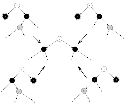
This program uses a ‘quick-sort’ like approach to re-arrange the array so that all the elements before lef t are less than or equal to m; while those between lef tandrightare greater thanm. This is shown in figure1.

x[i]<=m

x[i]>m

...?...

left

right

Figure 1: Divide the array, all x[i]≤mwhere 0≤i < lef t; while allx[i]> m wherelef t≤i < right. The left elements are unknown.

This program is fast and it doesn’t need extra stack space. However, com-pared to the previous Haskell program, it’s hard to read and the expressiveness decreased. We have to balance performance and expressiveness.

3_{This is done automatically in most functional languages since our function is in tail}

(18)

0.3 The number puzzle, power of data structure

If the first problem, to find the minimum free number, is a some what useful in practice, this problem is a ‘pure’ one for fun. The puzzle is to find the 1,500th number, which only contains factor 2, 3 or 5. The first 3 numbers are of course 2, 3, and 5. Number 60 = 22₃1₅1_{, However it is the 25th number. Number}

21 = 20₃1₇1_{, isn’t a valid number because it contains a factor 7. The first 10}

such numbers are list as the following. 2,3,4,5,6,8,9,10,12,15

If we consider 1 = 20₃0₅0_{, then 1 is also a valid number and it is the first}

one.

0.3.1 The brute-force solution

It seems the solution is quite easy without need any serious algorithms. We can check all numbers from 1, then extract all factors of 2, 3 and 5 to see if the left part is 1.

1: function_Get-Number(n) 2: x←1

3: i←0 4: loop

5: if Valid?(x)then

6: i←i+ 1

7: if i=nthen

8: returnx

9: x←x+ 1 10: functionValid?(x) 11: whilexmod 2 = 0do

12: x←x/2

13: whilexmod 3 = 0do

14: x←x/3

15: whilexmod 5 = 0do

16: x←x/5

17: if x= 1then 18: returnT rue 19: else

20: returnF alse

This ‘brute-force’ algorithm works for most small n. However, to find the 1500th number (which is 859963392), the C program based on this algorithm takes 40.39 seconds in my computer. I have to kill the program after 10 minutes when I increasednto 15,000.

0.3.2 Improvement 1

(19)

0.3. THE NUMBER PUZZLE, POWER OF DATA STRUCTURE 19

We start from 1, and times it with 2, or 3, or 5 to generate rest numbers. The problem turns to be how to generate the candidate number in order? One handy way is to utilize the queue data structure.

A queue data structure is used to push elements at one end, and pops them at the other end. So that the element be pushed first is also be popped out first. This property is called FIFO (First-In-First-Out).

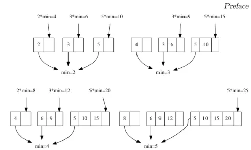
The idea is to push 1 as the only element to the queue, then we pop an element, times it with 2, 3, and 5, to get 3 new elements. We then push them back to the queue in order. Note that, the new elements may have already existed in the queue. In such case, we just drop the element. The new element may also smaller than the others in the queue, so we must put them to the correct position. Figure2illustrates this idea.

1

1*2=2 1*3=3 1*5=5

2 3 5

2*2=4 2*3=6 2*5=10

3 4 5 6 10

3*2=6 3*3=9 3*5=15

4 5 6 9 10 15

4*2=8 4*3=12 4*5=20

Figure 2: First 4 steps of constructing numbers with a queue. 1. Queue is initialized with 1 as the only element;

2. New elements 2, 3, and 5 are pushed back;

3. New elements 4, 6, and 10, are pushed back in order;

4. New elements 9 and 15 are pushed back, element 6 already exists.

This algorithm is shown as the following.

1: function_Get-Number(n) 2: Q←N IL

3: _Enqueue(Q,1)

4: whilen >0do

5: x←_Dequeue(Q)

6: _{Unique-Enqueue}(Q,2x)

7: _{Unique-Enqueue}(Q,3x)

8: Unique-Enqueue(Q,5x)

9: n←n−1 10: returnx

11: functionUnique-Enqueue(Q, x) 12: i←0

13: whilei <|Q| ∧Q[i]< x do 14: i←i+ 1

15: if i <|Q| ∧x=Q[i]then

16: return

(20)

The insert function takes O(|Q|) time to find the proper position and insert it. If the element has already existed, it just returns.

A rough estimation tells that the length of the queue increase proportion to n, (Each time, we extract one element, and pushed 3 new, the increase ratio≤ 2), so the total running time isO(1 + 2 + 3 +...+n) =O(n2).

Figure3 shows the number of queue access time against n. It is quadratic curve which reflect theO(n2) performance.

Figure 3: Queue access count v.s. n.

The C program based on this algorithm takes only 0.016[s] to get the right answer 859963392. Which is 2500 times faster than the brute force solution.

Improvement 1 can also be considered in recursive way. Suppose X is the infinity series for all numbers which only contain factors of 2, 3, or 5. The following formula shows an interesting relationship.

X ={1} ∪ {2x:∀x∈X} ∪ {3x:∀x∈X} ∪ {5x:∀x∈X} (2)

Where we can define ∪ to a special form so that all elements are stored in order as well as unique to each other. Suppose that X = {x1, x2, x3...},

Y ={y1, y2, y3, ...}, X′={x2, x3, ...}andY′ ={y2, y3, ...}. We have

X∪Y =

          

X : Y =ϕ Y : X=ϕ {x1, X′∪Y} : x1< y1

{x1, X′∪Y′} : x1=y1

{y1, X∪Y′} : x1> y1

In a functional programming language such as Haskell, which supports lazy evaluation, The above infinity series functions can be translate into the following program.

ns=1:merge (map (∗2) ns) (merge (map (∗3) ns) (map (∗5) ns))

merge [] l=l

merge l []=l

(21)

0.3. THE NUMBER PUZZLE, POWER OF DATA STRUCTURE 21

| x==y =x : merge xs ys

| otherwise=y : merge (x:xs) ys

By evaluate ns !! (n-1), we can get the 1500th number as below.

>ns !! (1500-1) 859963392

0.3.3 Improvement 2

Considering the above solution, although it is much faster than the brute-force one, It still has some drawbacks. It produces many duplicated numbers and they are finally dropped when examine the queue. Secondly, it does linear scan and insertion to keep the order of all elements in the queue, which degrade the ENQUEUE operation fromO(1) toO(|Q|).

If we use three queues instead of using only one, we can improve the solution one step ahead. Denote these queues asQ2,Q3, andQ5, and we initialize them

asQ2={2},Q3={3}andQ5={5}. Each time we DEQUEUEed the smallest

one fromQ2,Q3, andQ5as x. And do the following test:

• If xcomes fromQ2, we ENQUEUE 2x, 3x, and 5xback toQ2, Q3, and

Q5 respectively;

• If x comes from Q3, we only need ENQUEUE 3x to Q3, and 5x to Q5;

We needn’t ENQUEUE 2xtoQ2, because 2xhave already existed inQ3;

• Ifxcomes fromQ5, we only need ENQUEUE 5xtoQ5; there is no need

to ENQUEUE 2x, 3x to Q2, Q3 because they have already been in the

queues;

We repeatedly ENQUEUE the smallest one until we find then-th element. The algorithm based on this idea is implemented as below.

1: function_Get-Number(n) 2: if n= 1 then

3: return1

4: else

5: Q2← {2}

6: Q3← {3}

7: Q5← {5}

8: whilen >1 do

9: x←min(_Head(Q2),Head(Q3),Head(Q5))

10: if x=_Head(Q2)then

11: _Dequeue(Q2)

12: _Enqueue(Q2,2x)

13: _Enqueue(Q3,3x)

14: _Enqueue(Q5,5x)

15: else if x=_Head(Q3)then

16: _Dequeue(Q3)

17: Enqueue(Q3,3x)

18: Enqueue(Q5,5x)

19: else

(22)

2

min=2

3 5

2*min=4 3*min=6 5*min=10

4

min=3

3 6 5 10

3*min=9 5*min=15

4

min=4

6 9 5 10 15

2*min=8 3*min=12 5*min=20

8

min=5

6 9 12 5 10 15 20

5*min=25

Figure 4: First 4 steps of constructing numbers withQ2, Q3, andQ5.

1. Queues are initialized with 2, 3, 5 as the only element; 2. New elements 4, 6, and 10 are pushed back;

3. New elements 9, and 15, are pushed back; 4. New elements 8, 12, and 20 are pushed back; 5. New element 25 is pushed back.

21: _Enqueue(Q5,5x)

22: n←n−1

23: returnx

This algorithm loops n times, and within each loop, it extract one head element from the three queues, which takes constant time. Then it appends one to three new elements at the end of queues which bounds to constant time too. So the total time of the algorithm bounds to O(n). The C++ program translated from this algorithm shown below takes less than 1µs to produce the 1500th number, 859963392.

typedef unsigned long Integer;

Integer get_number(int n){ if(n==1)

return 1;

queue<Integer>Q2, Q3, Q5; Q2.push(2);

Q3.push(3); Q5.push(5); Integer x; while(n-->1){

x =min(min(Q2.front(), Q3.front()), Q5.front());

if(x==Q2.front()){

(23)

0.4. NOTES AND SHORT SUMMARY 23

Q5.push(x∗5); }

else if(x==Q3.front()){

Q3.pop(); Q3.push(x∗3); Q5.push(x∗5); }

else{ Q5.pop(); Q5.push(x∗5); }

}

return x; }

This solution can be also implemented in Functional way. We define a func-tiontake(n), which will return the firstnnumbers contains only factor 2, 3, or 5.

take(n) =f(n,{1},{2},{3},{5}) Where

f(n, X, Q2, Q3, Q5) =

{

X : n= 1 f(n−1, X∪ {x}, Q2′, Q′3, Q′5) : otherwise

x=min(Q21, Q31, Q51)

Q′₂, Q′₃, Q′₅=

  

{Q22, Q23, ...} ∪ {2x}, Q3∪ {3x}, Q5∪ {5x} : x=Q21

Q2,{Q32, Q33, ...} ∪ {3x}, Q5∪ {5x} : x=Q31

Q2, Q3,{Q52, Q53, ...} ∪ {5x} : x=Q51

And these functional definition can be realized in Haskell as the following.

ks 1 xs _=xs

ks n xs (q2, q3, q5)=ks (n-1) (xs++[x]) update

where

x=minimum $ map head [q2, q3, q5]

update | x==head q2 =((tail q2)++[x∗2], q3++[x∗3], q5++[x∗5])

| x==head q3 =(q2, (tail q3)++[x∗3], q5++[x∗5])

| otherwise=(q2, q3, (tail q5)++[x∗5])

takeN n=ks n [1] ([2], [3], [5])

Invoke ‘last takeN 1500’ will generate the correct answer 859963392.

0.4 Notes and short summary

If review the 2 puzzles, we found in both cases, the brute-force solutions are so weak. In the first problem, it’s quite poor in dealing with long ID list, while in the second problem, it doesn’t work at all.

(24)

Compare to what we learned in mathematics course in school, we haven’t been taught the method like this.

While there have been already a lot of wonderful books about algorithms, data structures and math, however, few of them provide the comparison between the procedural solution and the functional solution. From the above discussion, it can be found that functional solution sometimes is very expressive and they are close to what we are familiar in mathematics.

This series of post focus on providing both imperative and functional algo-rithms and data structures. Many functional data structures can be referenced from Okasaki’s book[6]. While the imperative ones can be founded in classic text books [2] or even in WIKIpedia. Multiple programming languages, includ-ing, C, C++, Python, Haskell, and Scheme/Lisp will be used. In order to make it easy to read by programmers with diﬀerent background, pseudo code and mathematical function are the regular descriptions of each post.

The author is NOT a native English speaker, the reason why this book is only available in English for the time being is because the contents are still changing frequently. Any feedback, comments, or criticizes are welcome.

0.5 Structure of the contents

In the following series of post, I’ll first introduce about elementary data tures before algorithms, because many algorithms need knowledge of data struc-tures as prerequisite.

The ‘hello world’ data structure, binary search tree is the first topic; Then we introduce how to solve the balance problem of binary search tree. After that, I’ll show other interesting trees. Trie, Patricia, suﬃx trees are useful in text manipulation. While B-trees are commonly used in file system and data base implementation.

The second part of data structures is about heaps. We’ll provide a gen-eral Heap definition and introduce about binary heaps by array and by explicit binary trees. Then we’ll extend to K-ary heaps including Binomial heaps, Fi-bonacci heaps, and pairing heaps.

Array and queues are considered among the easiest data structures typically, However, we’ll show how diﬃcult to implement them in the third part.

As the elementary sort algorithms, we’ll introduce insertion sort, quick sort, merge sort etc in both imperative way and functional way.

(25)

Bibliography

[1] Richard Bird. “Pearls of functional algorithm design”. Cambridge Univer-sity Press; 1 edition (November 1, 2010). ISBN-10: 0521513383

[2] Jon Bentley. “Programming Pearls(2nd Edition)”. Addison-Wesley Profes-sional; 2 edition (October 7, 1999). ISBN-13: 978-0201657883

[3] Chris Okasaki. “Purely Functional Data Structures”. Cambridge university press, (July 1, 1999), ISBN-13: 978-0521663502

[4] Thomas H. Cormen, Charles E. Leiserson, Ronald L. Rivest and Cliﬀord Stein. “Introduction to Algorithms, Second Edition”. The MIT Press, 2001. ISBN: 0262032937.

(26)

(27)

Part II

Trees

(28)

(29)

Chapter 1

Binary search tree, the

‘hello world’ data structure

1.1 Introduction

Arrays or lists are typically considered the ‘hello world’ data structures. How-ever, we’ll see they are not actually particularly easy to implement. In some procedural settings, arrays are the most elementary data structures, and it is possible to implement linked lists using arrays (see section 10.3 in [2]). On the other hand, in some functional settings, linked lists are the elementary building blocks used to create arrays and other data structures.

Considering these factors, we start with Binary Search Trees (or BST) as the ‘hello world’ data structure using an interesting problem Jon Bentley mentioned in ‘Programming Pearls’ [2]. The problem is to count the number of times each word occurs in a large text. One solution in C++ is below:

int main(int, char∗∗ ){

map<string, int>dict; string s;

while(cin>>s)

++dict[s];

map<string, int>::iterator it=dict.begin();

for(; it!=dict.end();++it)

cout<<it→first<<": "<<it→second<<"λn"; }

And we can run it to produce the result using the following UNIX commands 1_.

$ g++ wordcount.cpp -o wordcount $ cat bbe.txt | ./wordcount > wc.txt

The map provided in the standard template library is a kind of balanced BST with augmented data. Here we use the words in the text as the keys and the number of occurrences as the augmented data. This program is fast, and

1_{This is not a UNIX unique command, in Windows OS, it can be achieved by:} _type bbe.txt | wordcount.exe > wc.txt

(30)

it reflects the power of BSTs. We’ll introduce how to implement BSTs in this section and show how to balance them in a later section.

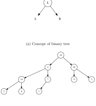
Before we dive into BSTs, let’s first introduce the more general binary tree. Binary trees are recursively defined. BSTs are just one type of binary tree. A binary tree is usually defined in the following way.

A binary tree is

• either an empty node;

• or a node containing 3 parts: a value, a left child which is a binary tree and a right child which is also a binary tree.

Figure 1.1shows this concept and an example binary tree.

k

L R

(a) Concept of binary tree

16

4 10

14 7

2 8 1

9 3

(b) An example binary tree

Figure 1.1: Binary tree concept and an example.

A BST is a binary tree where the following applies to each node:

• all the values in left child tree are less than the value of this node; • the value of this node is less than any values in its right child tree.

Figure 1.2shows an example of a BST. Comparing with Figure1.1, we can see the diﬀerences in how keys are ordered between them.

1.2 Data Layout

(31)

1.2. DATA LAYOUT 31

4

3 8

1

2

7 16

10

9 14

Figure 1.2: An example of a BST

The node first contains a field for the key, which can be augmented with satellite data. The next two fields contain pointers to the left and right children, respectively. To make backtracking to ancestors easy, a parent field is sometimes provided as well.

In this section, we’ll ignore the satellite data for the sake of simplifying the illustrations. Based on this layout, the node of BST can be defined in a procedural language, such as C++:

template<class T>

struct node{

node(T x):key(x), left(0), right(0), parent(0){} ~node(){

delete left; delete right; }

node∗ left;

node∗ right;

node∗ parent; //Optional, it’s helpful for succ and pred

T key; };

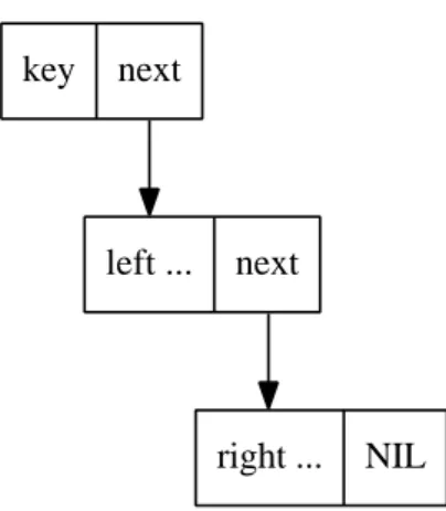
There is another setting, for instance in Scheme/Lisp languages, the elemen-tary data structure is a linked list. Figure1.4 shows how a BST node can be built on top of linked list.

In more functional settings, it’s hard to use pointers for backtracking (and typically, there is no need for backtracking, since there are usually top-down recursive solutions), and so the ‘parent’ field has been omitted in that layout.

(32)

key + satellite data

left

right

parent

key + satellite data

left

right

parent

key + satellite data

left

right

parent

...

Figure 1.3: Layout of nodes with parent field.

key

left ...

right ...

NIL

(33)

1.3. INSERTION 33

a BST node in Haskell:

data Tree a=Empty

| Node (Tree a) a (Tree a)

1.3 Insertion

To insert a keyk (sometimes along with a value in practice) to a BST T, we can use the following algorithm:

• If the tree is empty, construct a leaf node with key =k; • Ifkis less than the key of root node, insert it in the left child; • Ifkis greater than the key of root node, insert it in the right child.

The exception to the above is when k is equal to the key of the root node, meaning it already exists in the BST, and we can either overwrite the data, or just do nothing. To simplify things, this case has been skipped in this section.

This algorithm is described recursively. It’s simplicity is why we consider the BST structure the ‘hello world’ data structure. Formally, the algorithm can be represented with a recursive mathematical function:

insert(T, k) =

  

node(ϕ, k, ϕ) : T =ϕ node(insert(Tl, k), k′, Tr) : k < k′ node(Tl, k′, insert(Tr, k)) : otherwise

(1.1)

Where Tl is the left child, Tr is the right child, and k′ is the key when T isn’t empty.

The node function creates a new node given the left subtree, a key and a right subtree as parameters. ϕmeans NIL or empty.

Translating the above functions directly to Haskell yields the following pro-gram:

insert Empty k=Node Empty k Empty

insert (Node l x r) k | k <x=Node (insert l k) x r

| otherwise=Node l x (insert r k)

This program utilized the pattern matching features provided by the lan-guage. However, even in functional settings without this feature (e.g. Scheme/Lisp) the program is still expressive:

(define (insert tree x)

(cond ((null? tree) (list ’() x ’())) ((<x (key tree))

(make-tree (insert (left tree) x) (key tree)

(right tree))) ((>x (key tree))

(make-tree (left tree) (key tree)

(insert (right tree) x)))))

(34)

1: function_Insert(T, k) 2: root←T

3: x←Create-Leaf(k)

4: parent←N IL 5: whileT ̸=N ILdo 6: parent←T

7: if k <Key(T)then

8: T ←_Left(T)

9: else

10: T ←_Right(T)

11: _Parent(x)←parent

12: if parent=N ILthen ▷treeT is empty

13: returnx

14: else if k <Key(parent)then 15: Left(parent)←x

16: else

17: Right(parent)←x

18: returnroot

19: function_Create-Leaf(k)

20: x←_Empty-Node

21: _Key(x)←k 22: _Left(x)←N IL

23: Right(x)←N IL

24: Parent(x)←N IL

25: returnx

While more complex than the functional algorithm, it is still fast, even when presented with very deep trees. Complete C++ and python programs are avail-able along with this section for reference.

1.4 Traversing

Traversing means visiting every element one-by-one in a BST. There are 3 ways to traverse a binary tree: a pre-order tree walk, an in-order tree walk and a post-order tree walk. The names of these traversal methods highlight the order in which we visit the root of a BST.

• pre-order traversal:, visit the key, then the left child, finally the right child;

• in-order traversal: visit the left child, then the key, finally the right child;

• post-order traversal: visit the left child, then the right child, finally the key.

Note that each ‘visiting’ operation is recursive. As mentioned before, we see that the order in which the key is visited determines the name of the traversal method.

(35)

1.4. TRAVERSING 35

• pre-order traversal results: 4, 3, 1, 2, 8, 7, 16, 10, 9, 14;

• in-order traversal results: 1, 2, 3, 4, 7, 8, 9, 10, 14, 16;

• post-order traversal results: 2, 1, 3, 7, 9, 14, 10, 16, 8, 4.

The in-order walk of a BST outputs the elements in increasing order. The definition of a BST ensures this interesting property, while the proof of this fact is left as an exercise to the reader.

The in-order tree walk algorithm can be described as:

• If the tree is empty, just return;

• traverse the left child by in-order walk, then access the key, finally traverse the right child by in-order walk.

Translating the above description yields a generic map function:

map(f, T) =

{

ϕ : T =ϕ

node(T_l′, k′, T_r′) : otherwise (1.2) Where

T_l′=map(f, Tl) T_r′=map(f, Tr) k′=f(k)

AndTl, Tr andkare the children and key when the tree isn’t empty. If we only need access the key without create the transformed tree, we can realize this algorithm in procedural way lie the below C++ program.

template<class T, class F>

void in_order_walk(node<T>∗ t, F f){ if(t){

in_order_walk(t→left, f);

f(t→value);

in_order_walk(t→right, f);

} }

The function takes a parameter f, it can be a real function, or a function object, this program will apply f to the node by in-order tree walk.

We can simplified this algorithm one more step to define a function which turns a BST to a sorted list by in-order traversing.

toList(T) =

{

ϕ : T =ϕ

toList(Tl)∪ {k} ∪toList(Tr) : otherwise (1.3)

Below is the Haskell program based on this definition.

toList Empty=[]

(36)

This provides us a method to sort a list of elements. We can first build a BST from the list, then output the tree by in-order traversing. This method is called as ‘tree sort’. Let’s denote the list X={x1, x2, x3, ..., xn}.

sort(X) =toList(f romList(X)) (1.4) And we can write it in function composition form.

sort=toList.f romList

Where functionf romListrepeatedly insert every element to an empty BST.

f romList(X) =f oldL(insert, ϕ, X) (1.5) It can also be written in partial application form2 like below.

f romList=f oldL insert ϕ

For the readers who are not familiar with folding from left, this function can also be defined recursively as the following.

f romList(X) =

{

ϕ : X=ϕ insert(f romList({x2, x3, ..., xn}), x1) : otherwise

We’ll intense use folding function as well as the function composition and partial evaluation in the future, please refer to appendix of this book or [6] [7] and [8] for more information.

Exercise 1.1

• Given the in-order traverse result and porder traverse result, can you re-construct the tree from these result and figure out the post-order traversing result?

– Pre-order result: 1, 2, 4, 3, 5, 6;

– In-order result: 4, 2, 1, 5, 3, 6;

– Post-order result: ?

• Write a program in your favorite language to re-construct the binary tree from pre-order result and in-order result.

• Prove why in-order walk output the elements stored in a binary search tree in increase order?

• Can you analyze the performance of tree sort with big-O notation?

2_{Also known as ’Curried form’ to memorialize the mathematican and logician Haskell}

(37)

1.5. QUERYING A BINARY SEARCH TREE 37

1.5 Querying a binary search tree

There are three types of querying for binary search tree, searching a key in the tree, find the minimum or maximum element in the tree, and find the predecessor or successor of an element in the tree.

1.5.1 Looking up

According to the definition of binary search tree, search a key in a tree can be realized as the following.

• If the tree is empty, the searching fails;

• If the key of the root is equal to the value to be found, the search succeed. The root is returned as the result;

• If the value is less than the key of the root, search in the left child. • Else, which means that the value is greater than the key of the root, search

in the right child.

This algorithm can be described with a recursive function as below.

lookup(T, x) =

      

ϕ : T =ϕ T : k=x lookup(Tl, x) : x < k lookup(Tr, x) : otherwise

(1.6)

WhereTl,Trandkare the children and key whenT isn’t empty. In the real application, we may return the satellite data instead of the node as the search result. This algorithm is simple and straightforward. Here is a translation of Haskell program.

lookup Empty _=Empty

lookup t@(Node l k r) x | k ==x=t

| x <k=lookup l x

| otherwise=lookup r x

If the BST is well balanced, which means that almost all nodes have both non-NIL left child and right child, for n elements, the search algorithm takes O(lgn) time to perform. This is not formal definition of balance. We’ll show it in later post about red-black-tree. If the tree is poor balanced, the worst case takesO(n) time to search for a key. If we denote the height of the tree ash, we can uniform the performance of the algorithm asO(h).

The search algorithm can also be realized without using recursion in a pro-cedural manner.

1: function_Search(T, x)

2: whileT ̸=N IL∧_Key(T)̸=xdo 3: if x <_Key(T)then

4: T ←_Left(T)

5: else

6: T ←_Right(T)

(38)

Below is the C++ program based on this algorithm.

template<class T>

node<T>∗ search(node<T>∗ t, T x){ while(t && t→key!=x){

if(x <t→key) t=t→left; else t=t→right;

}

return t; }

1.5.2 Minimum and maximum

Minimum and maximum can be implemented from the property of binary search tree, less keys are always in left child, and greater keys are in right.

For minimum, we can continue traverse the left sub tree until it is empty. While for maximum, we traverse the right.

min(T) =

{

k : Tl=ϕ

min(Tl) : otherwise (1.7)

max(T) =

{

k : Tr=ϕ

max(Tr) : otherwise (1.8) Both functions bound to O(h) time, where his the height of the tree. For the balanced BST,min/maxare bound toO(lgn) time, while they areO(n) in the worst cases.

We skip translating them to programs, It’s also possible to implement them in pure procedural way without using recursion.

1.5.3 Successor and predecessor

The last kind of querying is to find the successor or predecessor of an element. It is useful when a tree is treated as a generic container and traversed with iterator. We need access the parent of a node to make the implementation simple.

It seems hard to find the functional solution, because there is no pointer like field linking to the parent node3_{. One solution is to left ‘breadcrumbs’ when we} visit the tree, and use these information to back-track or even re-construct the whole tree. Such data structure, that contains both the tree and ‘breadcrumbs’ is called zipper. please refer to [9] for details.

However, If we consider the original purpose of providingsucc/predfunction, ‘to traverse all the BST elements one by one‘ as a generic container, we realize that they don’t make significant sense in functional settings because we can traverse the tree in increase order bymapfunction we defined previously.

We’ll meet many problems in this series of post that they are only valid in imperative settings, and they are not meaningful problems in functional settings at all. One good example is how to delete an element in red-black-tree[3].

In this section, we’ll only present the imperative algorithm for finding the successor and predecessor in a BST.

(39)

1.5. QUERYING A BINARY SEARCH TREE 39

When finding the successor of element x, which is the smallest one y that satisfiesy > x, there are two cases. If the node with valuexhas non-NIL right child, the minimum element in right child is the answer; For example, in Figure

1.5, in order to find the successor of 8, we search it’s right sub tree for the minimum one, which yields 9 as the result. While if node x don’t have right child, we need back-track to find the closest ancestor whose left child is also ancestor ofx. In Figure1.5, since 2 don’t have right sub tree, we go back to its parent 1. However, node 1 don’t have left child, so we go back again and reach to node 3, the left child of 3, is also ancestor of 2, thus, 3 is the successor of node 2.

4

3 8

1

2

7 16

10

9 14

Figure 1.5: The successor of 8, is the minimum one in its right sub tree, 9; In order to find the successor of 2, we go up to its parent 1, but 1 doesn’t have left child, we go up again and find 3. Because its left child is also the ancestor of 2, 3 is the result.

Based on this description, the algorithm can be given as the following.

1: function_Succ(x)

2: if _Right(x)̸=N ILthen

3: return_Min(_Right(x)) 4: else

5: p←Parent(x)

6: whilep̸=N ILandx=Right(p)do

7: x←p

8: p←Parent(p)

9: returnp

Ifxdoesn’t has successor, this algorithm returns NIL. The predecessor case is quite similar to the successor algorithm, they are symmetrical to each other.

1: function_Pred(x)

2: if Left(x)̸=N ILthen 3: returnMax(Left(x)) 4: else

(40)

6: while p̸=N ILandx=_Left(p)do

7: x←p

8: p←Parent(p)

9: returnp

Below are the Python programs based on these algorithms. They are changed a bit in while loop conditions.

def succ(x):

if x.right is not None: return tree_min(x.right)

p =x.parent

while p is not None and p.left !=x:

x=p

p=p.parent

return p

def pred(x):

if x.left is not None: return tree_max(x.left)

p =x.parent

while p is not None and p.right !=x:

x=p

p=p.parent

return p

Exercise 1.2

• Can you figure out how to iterate a tree as a generic container by using

Pred/Succ? What’s the performance of such traversing process in terms of big-O?

• A reader discussed about traversing all elements inside a range [a, b]. In C++, the algorithm looks like the below code:

for each (m.lower bound(12), m.upper bound(26), f);

Can you provide the purely function solution for this problem?

1.6 Deletion

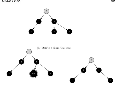
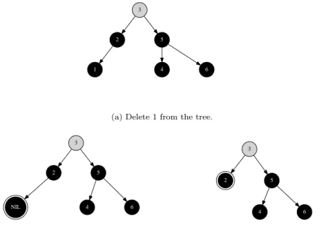
Deletion is another ‘imperative only’ topic for binary search tree. This is because deletion mutate the tree, while in purely functional settings, we don’t modify the tree after building it in most application.

However, One method of deleting element from binary search tree in purely functional way is shown in this section. It’s actually reconstructing the tree but not modifying the tree.

Deletion is the most complex operation for binary search tree. this is because we must keep the BST property, that for any node, all keys in left sub tree are less than the key of this node, and they are all less than any keys in right sub tree. Deleting a node can break this property.

In this post, diﬀerent with the algorithm described in [2], A simpler one from SGI STL implementation is used.[6]

(41)

1.6. DELETION 41

• Ifxhas no child or only one child, splice x out;

• Otherwise (xhas two children), use minimum element of its right sub tree to replacex, and splice the original minimum element out.

The simplicity comes from the truth that, the minimum element is stored in a node in the right sub tree, which can’t have two non-NIL children. It ends up in the trivial case, the node can be directly splice out from the tree.

Figure1.6, 1.7, and1.8illustrate these diﬀerent cases when deleting a node from the tree.

Tree

x

NIL NIL

Figure 1.6: xcan be spliced out.

Tree

x

L NIL

(a) Before deletex.

Tree

L

(b) After delete x, x is spliced out, and replaced by its left child.

Tree

x

NIL R

(c) Before deletex.

Tree

R

(d) After delete x, x is spliced out, and replaced by its right child.

(42)

Tree

x

L R

(a) Before deletex.

Tree

min(R)

L delete(R, min(R))

(b) After delete x,x is replaced by splicing the minimum element from its right child.

Figure 1.8: Delete a node which has both children.

Based on this idea, the deletion can be defined as the below function.

delete(T, x) =

              

ϕ : T =ϕ node(delete(Tl, x), K, Tr) : x < k

node(Tl, k, delete(Tr, x)) : x > k

Tr : x=k∧Tl=ϕ Tl : x=k∧Tr=ϕ node(Tl, y, delete(Tr, y)) : otherwise

(1.9)

Where

Tl=lef t(T) Tr=right(T) k=key(T) y=min(Tr)

Translating the function to Haskell yields the below program.

delete Empty _=Empty

delete (Node l k r) x | x<k=(Node (delete l x) k r)

| x>k=(Node l k (delete r x))

-- x ==k

| isEmpty l=r

| isEmpty r=l

| otherwise=(Node l k’ (delete r k’))

where k’=min r

(43)

1.6. DELETION 43

It’s also possible to pass the node but not the element to the algorithm for deletion. Thus the searching is no more needed.

The imperative algorithm is more complex because it need set the parent properly. The function will return the root of the result tree.

1: function_Delete(T, x) 2: r←T

3: x′ ←x ▷ savex

4: p←_Parent(x)

5: if _Left(x) =N ILthen

6: x←_Right(x)

7: else if Right(x) =N ILthen 8: x←Left(x)

9: else ▷both children are non-NIL

10: y←Min(Right(x))

11: Key(x)←Key(y)

12: Copy other satellite data fromy tox

13: if _Parent(y)̸=xthen ▷ yhasn’t left sub tree

14: _Left(_Parent(y))←_Right(y)

15: else ▷ y is the root of right child ofx

16: _Right(x)←_Right(y)

17: Removey 18: returnr 19: if x̸=N ILthen

20: Parent(x)←p

21: if p=N ILthen ▷We are removing the root of the tree

22: r←x

23: else

24: if _Left(p) =x′ then

25: _Left(p)←x

26: else

27: _Right(p)←x

28: Removex′ 29: returnr

Here we assume the node to be deleted is not empty (otherwise we can simply returns the original tree). In other cases, it will first record the root of the tree, create copy pointers tox, and its parent.

If either of the children is empty, the algorithm just splice xout. If it has two non-NIL children, we first located the minimum of right child, replace the key ofxtoy’s, copy the satellite data as well, then spliceyout. Note that there is a special case thaty is the root node ofx’s right sub tree.

Finally we need reset the stored parent if the originalx has only one non-NIL child. If the parent pointer we copied before is empty, it means that we are deleting the root node, so we need return the new root. After the parent is set properly, we finally remove the oldxfrom memory.

The relative Python program for deleting algorithm is given as below. Be-cause Python provides GC, we needn’t explicitly remove the node from the memory.

(44)

if x is None: return t

[root, old_x, parent] =[t, x, x.parent]

if x.left is None:

x=x.right

elif x.right is None:

x=x.left

else:

y=tree_min(x.right)

x.key=y.key

if y.parent !=x:

y.parent.left=y.right

else:

x.right=y.right

return root if x is not None:

x.parent=parent

if parent is None:

root=x

else:

if parent.left==old_x:

parent.left=x

else:

parent.right=x

return root

Because the procedure seeks minimum element, it runs in O(h) time on a tree of heighth.

Exercise 1.3

• There is a symmetrical solution for deleting a node which has two non-NIL children, to replace the element by splicing the maximum one out oﬀ the left sub-tree. Write a program to implement this solution.

1.7 Randomly build binary search tree

It can be found that all operations given in this post bound toO(h) time for a tree of heighth. The height aﬀects the performance a lot. For a very unbalanced tree,htends to beO(n), which leads to the worst case. While for balanced tree, hclose toO(lgn). We can gain the good performance.

How to make the binary search tree balanced will be discussed in next post. However, there exists a simple way. Binary search tree can be randomly built as described in [2]. Randomly building can help to avoid (decrease the possibility) unbalanced binary trees. The idea is that before building the tree, we can call a random process, to shuﬄe the elements.

Exercise 1.4

(45)

Bibliography

[1] Thomas H. Cormen, Charles E. Leiserson, Ronald L. Rivest and Cliﬀord Stein. “Introduction to Algorithms, Second Edition”. ISBN:0262032937. The MIT Press. 2001

[2] Jon Bentley. “Programming Pearls(2nd Edition)”. Addison-Wesley Profes-sional; 2 edition (October 7, 1999). ISBN-13: 978-0201657883

[3] Chris Okasaki. “Ten Years of Purely Functional Data Structures”. http://okasaki.blogspot.com/2008/02/ten-years-of-purely-functional-data.html

[4] SGI. “Standard Template Library Programmer’s Guide”. http://www.sgi.com/tech/stl/

[5] http://en.literateprograms.org/Category:Binary search tree

[6] http://en.wikipedia.org/wiki/Foldl

[7] http://en.wikipedia.org/wiki/Function composition

[8] http://en.wikipedia.org/wiki/Partial application

[9] Miran Lipovaca. “Learn You a Haskell for Great Good! A Beginner’s Guide”. the last chapter. No Starch Press; 1 edition April 2011, 400 pp. ISBN: 978-1-59327-283-8

(46)

(47)

Chapter 2

The evolution of insertion

sort

2.1 Introduction

In previous chapter, we introduced the ’hello world’ data structure, binary search tree. In this chapter, we explain insertion sort, which can be think of the ’hello world’ sorting algorithm1_{. It’s straightforward, but the performance} is not as good as some divide and conqueror sorting approaches, such as quick sort and merge sort. Thus insertion sort is seldom used as generic sorting utility in modern software libraries. We’ll analyze the problems why it is slow, and trying to improve it bit by bit till we reach the best bound of comparison based sorting algorithms,O(nlgn), by evolution to tree sort. And we finally show the connection between the ’hello world’ data structure and ’hello world’ sorting algorithm.

The idea of insertion sort can be vivid illustrated by a real life poker game[2]. Suppose the cards are shuﬄed, and a player starts taking card one by one.

At any time, all cards in player’s hand are well sorted. When the player gets a new card, he insert it in proper position according to the order of points. Figure2.1shows this insertion example.

Based on this idea, the algorithm of insertion sort can be directly given as the following.

function_Sort(A) X ←ϕ

foreachx∈Ado

Insert(X, x) returnX

It’s easy to express this process with folding, which we mentioned in the chapter of binary search tree.

insert=f oldL insert ϕ (2.1)

1_{Some reader may argue that ’Bubble sort’ is the easiest sort algorithm. Bubble sort isn’t}

(48)

Figure 2.1: Insert card 8 to proper position in a deck.

Note that in above algorithm, we store the sorted result inX, so this isn’t in-place sorting. It’s easy to change it to in-in-place algorithm. Denote the sequence asA={a1, a2, ..., an}.

function_Sort(A) fori←2 to|A|do

insertai to sorted sequence{a′₁, a′₂, ..., a′_i₋₁}

At any time, when we process the i-th element, all elements beforei have already been sorted. we continuously insert the current elements until consume all the unsorted data. This idea is illustrated as in figure 9.3.

... sorted elements ...

x

insert

... unsorted elements ...

Figure 2.2: The left part is sorted data, continuously insert elements to sorted part.

We can find there is recursive concept in this definition. Thus it can be expressed as the following.

sort(A) =

{

ϕ : A=ϕ insert(sort({a2, a3, ...}), a1) : otherwise

(2.2)

2.2 Insertion

We haven’t answered the question about how to realize insertion however. It’s a puzzle how does human locate the proper position so quickly.

(49)

2.2. INSERTION 49

function_Sort(A)

fori←2 to|A|do ▷InsertA[i] to sorted sequenceA[1...i−1] x←A[i]

j←i−1

whilej >0∧x < A[j] do A[j+ 1]←A[j]

j←j−1 A[j+ 1]←x

One may think scan from left to right is natural. However, it isn’t as eﬀect as above algorithm for plain array. The reason is that, it’s expensive to insert an element in arbitrary position in an array. As array stores elements continuously, if we want to insert new elementxin positioni, we must shift all elements after i, includingi+ 1, i+ 2, ...one position to right. After that the cell at positioni is empty, and we can putxin it. This is illustrated in figure2.3.

A[1] A[2] ... A[i-1] A[i] A[i+1] A[i+2] ... A[n-1] A[n] empty

x

insert

Figure 2.3: Insertxto array Aat positioni.

If the length of array isn, this indicates we need examine the firstielements, then perform n−i+ 1 moves, and then insert xto thei-th cell. So insertion from left to right need traverse the whole array anyway. While if we scan from right to left, we examineielements at most, and perform the same amount of moves.

Translate the above algorithm to Python yields the following code.

def isort(xs):

n=len(xs)

for i in range(1, n):

x =xs[i]

j =i - 1

while j ≥ 0 and x <xs[j]:

xs[j+1]=xs[j]

j=j - 1

xs[j+1]=x

It can be found some other equivalent programs, for instance the following ANSI C program. However this version isn’t as eﬀective as the pseudo code.

void isort(Key∗ xs, int n){

int i, j;

for(i=1; i<n;++i)

for(j=i-1; j≥0 && xs[j+1]<xs[j]; --j)

swap(xs, j, j+1);

Elementary Algorithms - Free Computer, Programming, Mathematics, Technical Books, Lecture Notes and Tutorials