THESIS
submitted in partial fulfillment of the requirements for the degree of
BACHELOR OF SCIENCE
in PHYSICS
Author : I.R. Berkman
Student ID : 1230638
Supervisor : Prof. Dr. Ir. T.H. Oosterkamp
2ndcorrector : Prof. Dr. M. Allan
I.R. Berkman
Huygens-Kamerlingh Onnes Laboratory, Leiden University P.O. Box 9500, 2300 RA Leiden, The Netherlands
August 18, 2015
Abstract
A new dipstick is built for the Lead Zeppelin project but with elliptical coils. We want to find the harmonic potential of this new
1 Introduction 1
1.1 MRFM 1
1.2 New Sensors using Magnetic Levitation 1
1.2.1 Benefits of using Elliptical Coils 2
1.3 Goals 2
2 Theory 3
2.1 Magnetic Fields 3
2.1.1 Magnetic Flux 3
2.1.2 The Biot-Savart Law 5
2.1.3 On-Axis Magnetic Field of Circular Coils in an
AH-Configuration 5
2.1.4 Off-axis Magnetic Field of Circular Coils in an
AH-Configuration 8
2.1.5 Off-axis Magnetic Field of Elliptical Coils in an
AH-Configuration 10
2.2 Superconductivity 12
2.2.1 Characteristics of Superconductors 12
2.2.2 Superconductor in a Magnetic Field 12
2.2.3 Resonance Frequencies of a Sphere 13
2.2.4 Resonance Frequencies of a Cube 14
2.2.5 Mixing Frequencies 16
2.2.6 Double Frequencies 19
3 Materials and Methods 21
3.1 The Circuit 21
3.1.2 The Switch 22
3.1.3 Twisting Wires 24
3.2 The Elliptical Coils 26
3.2.1 Winding the Coils 26
3.2.2 Assembling the Coils 28
3.3 The Big Coil 30
3.3.1 The Machine 30
3.3.2 Making the Big Coil 31
3.4 The Lead Particles 34
3.5 Preparing the Dipstick 36
4 Numerical Calculations and Predictions 41
4.1 The Magnetic Field 41
4.2 Approximating the Magnetic Field 47
4.3 Resonance Frequencies 50
4.3.1 Translational Frequencies 50
4.3.2 Rotational Frequencies 52
5 Results and Discussion 53
5.1 The Lead Zeppelin Experiment 53
5.2 Numerical Results 54
5.3 Fourier Spectrum of the Spherical Lead Zeppelin with
Cir-cular Coils 55
6 Conclusions 59
7 Follow up Experiments and Improvements 61
Chapter
1
Introduction
1.1
MRFM
Magnetic Resonance Force Microscopy (MRFM) is a technique which uses Atomic Force Microscopy (AFM) and Magnetic Resonance Imaging (MRI) to obtain images at nanometer scales.
The MRFM technique uses an ultrathin silicon cantilever with a ferromag-netic (iron cobalt) tip. Because an electron has a magferromag-netic property called ”spin”, it can attract or deflect the magnetic tip depending on the spin-position. The spins are repeatedly flipped by a high-frequency magnetic field induced by a coil. The result is that the cantilever oscillates due to the repelling and attracting forces of the flipping spins. By monitoring the cantilever oscillation with an interferometer while the sample moves underneath the cantilever creates data for a two of three dimensional re-construction. These measurements are usually performed at low temper-atures to reduce the noise of Brownian motions[1].
1.2
New Sensors using Magnetic Levitation
the cantilever, therefore the measurements will be more accurate when these energy losses are decreased or even better, removed.
A ingenious solution was published by Romero-Isart in his article “Quan-tum Magnetomechanics with Levitating Superconducting Microspheres”[2]. A superconducting particle is trapped in an anti-Helmholtz configuration. Because the potential is zero in the middle of the configuration, the super-conductor tends to stay there due to the Meissner effect[3]. This system has no mechanical energy losses which allows it to have a higher Q factor, a measure for the quality of an oscillating device, than ever before. More information about specifically these kinds of sensors can be found in ”The Lead Zeppelin Project” by M. De Wit[4].
1.2.1
Benefits of using Elliptical Coils
The original Lead Zeppelin project consisted of a small spherical piece of lead trapped in between two circular coils with repelling magnetic fields. The lead in this system has 6 degrees of freedom, where three are transla-tional and three rotatransla-tional. Because the field is symmetric in the x=0 and y=0 plane it becomes hard to distinguish the two translational frequencies in the x and y direction. Also, due to symmetry, the rotational frequency is immeasurable. This is more thoroughly explained in the ”Theory” chap-ter.
A way to distinguish the translational frequencies better is by making the magnetic field more asymmetrical. The most practical form is the elliptic one, which is just a squeezed circle. By using two elliptical coils we can now find which frequencies correspond to the translation frequency in the x and y direction. The rotational frequencies can be found by making the Zeppelin aspherical.
1.3
Goals
• Making the Lead Zeppelin with elliptical coils
• Finding the corresponding frequencies
• Finding the Q factor
Chapter
2
Theory
2.1
Magnetic Fields
2.1.1
Magnetic Flux
Flux is a key concept when talking about magnetic fields. In electromag-netism, the magnetic flux Φis the surface integral of the normal compo-nent of the magnetic field~B passing through that surface, or in equation-form:
Φ=
Z Z
~B·d~S (2.1)
When reading through this thesis, you will often find the word ”twisted wires” and this has everything to do with flux.
Say, for instance, that we have a closed circuit with area A.
+
-V A
in flux will induce an electromotive force or EMF which is given by
EMF=−dΦ
dt (2.2)
And because EMF is measured in voltage, the total voltage over the circuit will be different than the voltage of the source.
In present-day circuits, we almost never calculate with these kind of noise fluxes because they are too small to make any significant differences. How-ever, when we zoom in into a quantum scale these noises can become dis-astrous.
We can solve this by giving this wire a twist in the middle as seen below.
+ -V
Flux in
Flux out
Let us assume that both sides have an equal area and the magnetic field is a constant. The flux is then the same on both sides. But because of the twist, the twoA~ vectors will have opposite sign and the fluxes will cancel, resulting in a zero EMF.
2.1.2
The Biot-Savart Law
The Biot-Savart Law helps us calculating magnetic fields. Almost all the equations in this experiment can be derived from this law:
~B(~r) = µ0
4π
Z
~ I×r
ˆr
2 dl0 = µ0
4πI
Z
d~l0×~
r
r
3 (2.3)Where the constantµ0is called the permeability of free space:
µ0 =4π×10−7N/A2 (2.4)
The integration is along the path of the current~I. This path consists of the infinitesimal small dl0. The script r ”~
r
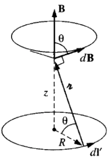
” is the vector from the current source to the point~r. The resulting magnetic field is given in Tesla.Figure 2.1: The elements of the Biot-Savart law in a sketch taken from Griffths’ ”Introduction to Electrodynamics”[5]
2.1.3
On-Axis Magnetic Field of Circular Coils in an
AH-Configuration
One of the easiest examples of the Biot-Savart law (equation 2.3) in use is the on-axis magnetic field of a round current loop.
Figure 2.2: The elements for calculating the on-axis magnetic field of a circular current loop
The cross product of d~l0 and ~
r
is in the direction of the d~B as shown in the figure. As we integrate d~l0 around the loop, d~B sweeps out a cone.Because of the circular symmetry, the horizontal components cancel and
the resulting ~B points only upward. This means we only have to look
at the vertical component of d~B which is cos(θ)d~B. The Biot-Savart law
becomes
B(z) = µ0
4πI
Z
d~l0
r
2cosθ = µ0I 4π cosθr
2Z
d~l0. (2.5)
The cosθand
r
are constants so we place these in front of the integral, sowe only have to integrate over d~l0. The path is over a circle so the path integral becomes the circumference 2πR. The field becomes:
B(z) = µ0I
4π
cosθ
r
2
2πR= µ0I
2
R2
(R2+z2)3/2. (2.6)
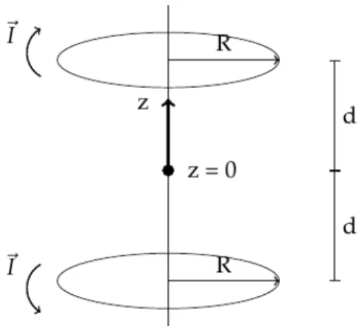
We now place two circular loops at distancez = d and z = −d as shown
Figure 2.3:An anti-Helmholtz configuration
This means that for the loop atz = −d the equation for the on-axis mag-netic field (equation 2.6) will be the same except now the variablezis sub-stituted forz+d. For the loop atz = dthe substitution will bez−dand the field will be negative because of the opposite current flow.
We can then add these two magnetic fields to get the total on-axis magnetic field at distancezof the origin:
B(z) = µ0IR
2
2
1
(R2+ (z+d)2)3/2 −
1
(R2+ (z−d)2)3/2
(2.7)
We can approximate the magnetic field of a coil by overlapping the loop n times on the same position of the loop, where n is the number of windings. The equation for two opposite placed coils with both the same number of windings will then be:
Bcoils(z) =n·
µ0IR2
2
1
(R2+ (z+d)2)3/2 −
1
(R2+ (z−d)2)3/2
(2.8)
2.1.4
Off-axis Magnetic Field of Circular Coils in an
AH-Configuration
Calculating the off-axis field of a circular loop at point~rbreaks some sym-metry and therefore requires more use of the elements of the Biot-Savart law (equation 2.3). We will look at the elliptical coil hereafter so it is better to calculate it in Cartesian coordinates instead of cylindrical.
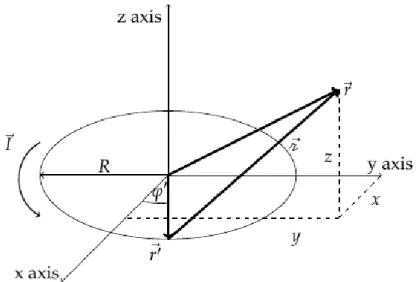
Figure 2.4:Off-axis magnetic field of a circular current loop
The point~ris where we want to calculate the magnetic field and the point
~r0 describes the path of the current flow. Both in Cartesian coordinates are
~r=
x y z and
~r0 =
Rcosϕ0
Rsinϕ0
0
. (2.9)
A segment d~l0 is basically the same as d~r0 and can be found by d~r
0
dϕ0dϕ
0.
The vector~
r
is equal to the vector difference~r−~r0, so we getd~l0 =
−Rsinϕ0
Rcosϕ0
0
dϕ
0
and ~
r
=
x−Rcosϕ0
y−Rsinϕ0
z
The integral of Biot-Savart law requires the cross product d~l0×~
r
:d~l0×~
r
=
zRcosϕ0
zRsinϕ0
R2−yRsinϕ0−xRcosϕ0
dϕ
0
(2.11)
and it requires
r
3:r
3 = (~r
·~r
)3/2 = (x2+y2+z2+R2−2xRcosϕ0−2yRsinϕ0)3/2
(2.12)
Combining 2.11 and 2.12 gives us the magnetic field
Bx(~r) = µ0IRz
4π
Z
2π0
cosϕ0
r
3 dϕ0
(2.13)
By(~r) = µ0IRz
4π
Z
2π0
sinϕ0
r
3 dϕ0
(2.14)
Bz(~r) = µ0IR
4π
Z
2π0
R−xcosϕ0−ysinϕ0
r
3 dϕ0
(2.15)
We have seen in section 2.1.3 that going from one loop to two opposite placed loops is just a matter of substituting z for z+d and z−d. The magnetic field at point~rfor an anti-Helmholtz configuration with coils of
nnumber of windings will be
Bx(~r) = µ0IRn
4π
Z
2π0
(z+d)
r
3 +−(z−d)
r
3−
cosϕ0dϕ0 (2.16)
By(~r) = µ0IRn
4π
Z
2π0
(z+d)
r
3 +−(z−d)
r
3−
sinϕ0dϕ0 (2.17)
Bz(~r) = µ0IRn
4π
Z
2π0 1
r
3 + − 1r
3 −(1−xRcosϕ0−yRsinϕ0)dϕ0 (2.18)
With
r
3+ = (x2+y2+ (z+d)2+R2−2xRcosϕ0−2yRsinϕ0)3/2 (2.19)
r
32.1.5
Off-axis Magnetic Field of Elliptical Coils in an
AH-Configuration
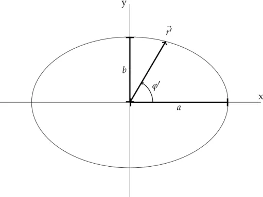
Elliptical current loops will have different field lines in the x and y direc-tion. In figure 2.5 we see that the radius constantRfor a circular loop has taken place for two constants: aandb. The constantais the distance from the centre to the ellipse along the x axis, the constantb the distance from the centre to the ellipse along the y axis.
x y
b
a ~r0
ϕ0
Figure 2.5:The elliptical loop in the z = 0 plane
The only difference in calculating the magnetic field of the elliptical loop is that the coordinates of~r0now become
~r0 =
acosϕ0
bsinϕ0
0
(2.21)
Bx(~r) = µ0Ibn
4π
Z
2π0
(
z+d)
r
3 +−(z−d)
r
3−
cosϕ0dϕ0 (2.22)
By(~r) = µ0Ian
4π
Z
2π0
(z+d)
r
3 +−(z−d)
r
3−
sinϕ0dϕ0 (2.23)
Bz(~r) = µ0In
4π
Z
2π0 1
r
3 + − 1r
3 −ab−bxcosϕ0−aysinϕ0
dϕ0 (2.24)
Where
r
3+ = (x2+y2+ (z+d)2+a2cos2ϕ0+b2sin2ϕ0−2axcosϕ0−2bysinϕ0)3/2
(2.25)
r
3− = (x2+y2+ (z−d)2+a2cos2ϕ0+b2sin2ϕ0−2axcosϕ0−2bysinϕ0)3/2
(2.26)
Note how substituting bothaand bforRgives the same equations as the circular magnetic fields.
2.2
Superconductivity
2.2.1
Characteristics of Superconductors
Superconductors are elements, inter-metallic alloys, or compounds that conduct electricity with zero resistance below a certain temperature and external magnetic field.[6]
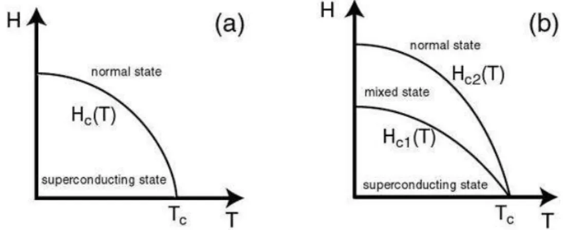
There are two types of superconductors: type I and type II. Type II usually have higher critical fields than type I superconductors.
Figure 2.6: Critical magnetic field as a function of temperature for (a) type I su-perconductors and (b) type II susu-perconductors. [7]
In this experiment two types of conducting wires are being used: a type II niobium and a type II niobium-titanium. Niobium has a critical tempera-ture of 9.2 Kelvin [8] and niobium-titanium at 10 Kelvin. [9]
The particle floating in the anti-Helmholtz configuration is made of pure lead which is a type I and has a critical temperature of 7.3 Kelvin. [10]
2.2.2
Superconductor in a Magnetic Field
The total force on a superconductor in a magnetic field is given by the equation 2.27 found in ”Local model for magnet-superconductor mechan-ical interaction: Experimental verification” by E. Diez-Jimenez et al. [11]
~F =
I
Where the surface integral encloses the surface of the superconducting particle. The vector~nis the normal on the surface and H~ is the magnetic field strength ~H = ~B/µ0−M~ , where ~B is the extern magnetic field. We
work in vacuum so we assume M~ = 0 which results in a magnetic field
~Bext =µ0H~ext.
Equation 2.27 can then be rewritten as:
~F =− 2
µ0
I
~n||~B||2−~
B(~n·~B)
dS. (2.28)
2.2.3
Resonance Frequencies of a Sphere
The force on a spherical particle in an anti-Helmholtz configuration with circular coils has been calculated in the thesis ”Beweging van een supergelei-dende bol in een anti-Helmholtz-configuratie by T. de Jong and D. Kok.[12]
~F(r,z) = −6πa3µ0n2I2R4d2
(R2+d2)5 (rrˆ+4zzˆ) (2.29)
This is equal to the equation of motion of an harmonic oscillator. The spring constants are:
kr = 6π
a3µ0n2I2R4d2
(R2+d2)5 andkz =
24πa3µ0n2I2R4d2
(R2+d2)5 (2.30)
And we get the omega out of the spring constant by:
ω =
r
k
m (2.31)
So the resulting omegas are:
ωr =nIR2d
s
6πr3µ0
m(R2+d2)5 andωz =2nIR 2d
s
6πr3µ0
m(R2+d2)5 (2.32)
We see that ωz = 2ωr. This means that the frequency peak for the
trans-lation z frequency is found at two times the frequencies in the x and y direction.
For the Lead Zeppelin with elliptical coils we can approximate the mag-netic field as:
~B(x,y,z) = axxˆ+byyˆ+czzˆ (2.33)
Where we need to compute a, b and c because the Taylor expansion is
analytically hard to do.
Using the same approximations as in the thesis gives us the following force:
~F(x,y,z) =−8πr3
3µ0 (a
2xxˆ+b2yyˆ+c2zzˆ) =
−2V µ0(a
2xxˆ+b2yyˆ+c2zzˆ)
(2.34)
And the following frequencies:
ωx =|a| ·
s
2V
µ0m =|a|
s
2
µ0ρ
ωy=|b| ·
s
2V
µ0m =|b|
s
2
µ0ρ
ωz =|c| ·
s
2V
µ0m =|c|
s
2
µ0ρ
(2.35)
Whereρis the density of lead.
2.2.4
Resonance Frequencies of a Cube
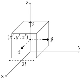
edges with a length of 2l and its center at (x0,y0,z0). The faces are in the same plane as the Cartesian planes.
z
y
x
2l
(x0,y0,z0)
ˆ z ˆ x ˆ y
Figure 2.7:A cube in Cartesian coordinates.
We start by splitting the integral 2.28 in two parts:
~F =− 2
µ0
I
~n||~B||2dS−
I
~B(~n·~B)dS
(2.36)
For the magnetic fields we use the approximation from equation 2.33 again. The front and the back plane (with normal vector ˆxand−xˆ) are calculated first.
The first part becomes:
I
~n||~B||2dS=
I
ˆ
x(a2x2+b2y2+c2y2)dS =
Z
y=l y=−lZ
z=l z=−l
a2(x0+l)2+b2y2+c2z2−a2(x0−l)2−b2y2−c2z2
ˆ
xdS=
Z
y=l y=−lZ
z=l z=−l4a2x0lxˆdS =4a2x0l·(2l)2xˆ =16a2l3x0xˆ =2Va2x0xˆ
The second integral:
I
~B(~n·~B)dS=· · · =
Z Z Z
Bx(~∇Bx)dV =
Z Z Z
a2xxˆdV = (2l)2
Z
x0+l x0−la2xxˆdx =
2a2l2xˆ·x2
x0+l x0−l
=8a2l3x0xˆ =Va2x0xˆ.
(2.38)
A more detailed derivation can be found in the thesis of T. De Jong and D. Kok [12]
Combining both integrals gives the solution of the force in x direction:
Fx(x0) =− 2 µ0(2Va
2x0−
Va2x0) = −2Va 2x0
µ0 (2.39)
The total force will be:
~F(x,y,z) =−2V
µ0(a
2xxˆ+b2yyˆ+c2zzˆ)
(2.40)
Which is exactly the same as equation 2.34, meaning that a superconduct-ing sphere and cube both have the same frequencies.
We can also see that this is the same force acting on a superconducting block with different lengs l1,l2,l3. The integrand in the first integral is
only a constant with a result depending only on the volume. In the second integral we can replace the limits withx0+l1 and x0−l1and see that the
result stays the same.
2.2.5
Mixing Frequencies
become important in the expansion. The complete expansion should look like:
Fx(x,y,z) =−axx−axxx2− · · · −ayy−ayyy2− · · · −azz−azzz2−. . .
−axyxy−axzxz−ayzyz−axxyx2y· · · =
− ∞
∑
nx=0∞
∑
ny=0∞
∑
nz=0a(nx,ny,nz)xnxynyznz
(2.41)
The solutions are not linear any more. This section and 2.2.6 are about these non-linearities.
In a Fourier spectrum we sometimes find the following frequencies as shown below:
Amplitude
Frequency 0
f1 f2
f2−f1 f2+ f1
Figure 2.8:Two frequencies with their corresponding mixing frequencies.
The frequencies at f2+f1and f2− f1are called mixed frequencies and are
caused by two signals multiplied together.
Let us assume two signalsx(t)andy(t)with the condition f2> f1:
x(t) = Acos(2πf1t) (2.42)
y(t) = Bcos(2πf2t). (2.43)
The product of the two signals become:
For the Fourier Transform we can use a little trick called the ”Convolution Theorem”. This theorem states that the Fourier transform of a product is equal to the convolution of the Fourier transform of each component:
F(x(t)·y(t)) = F(x(t))⊗ F(y(t)) (2.45) The convolution is an important tool in signal processing and is given by:
X(f)⊗Y(f) =
Z
∞−∞X( ˜
f)Y(f − f˜)d ˜f . (2.46)
Whereby the capital X is used from now on for the Fourier transform.
Anyhow, we still need to Fourier transform both signals apart, but this should be easy because the Fourier transform of a cosine is just two delta peaks.
Z
∞−∞
cos(2πf1t)e−2πi f tdt=
1 2
δ(f − f1) +δ(f + f1)
(2.47)
The Fourier Transform of both signals then become:
X(f) = A
Z
∞−∞cos(2πf1t)e
−2πi f tdt = A
2
δ(f −f1) +δ(f + f1)
(2.48)
Y(f) = B
Z
∞−∞
cos(2πf2t)e−2πi f tdt =
B
2
δ(f − f2) +δ(f + f2)
. (2.49)
Putting this in the convolution integral 2.46 gives:
X(f)⊗Y(f) =AB
4
Z
∞−∞
δ(f˜−f1) +δ(f˜+ f1)
δ(f − f2− f˜) +δ(f + f2− f˜)
d ˜f. (2.50)
AB
4
Z
∞−∞
δ(f˜− f1) +δ(f˜+ f1)
δ(f − f2−f˜)d ˜f (2.51)
+AB
4
Z
∞−∞
δ(f˜− f1) +δ(f˜+ f1)
δ(f + f2−f˜)d ˜f. (2.52)
Using the property of the Dirac-delta:
Z
∞−∞X( ˜
f)δ(f − f˜)d ˜f =X(f), (2.53)
the answer to the whole Fourier Transform becomes:
AB
4
δ(f − f1− f2) +δ(f + f1− f2) +δ(f − f1+ f2) +δ(f +f1+ f2)
.
(2.54)
We only want to look at the positive frequencies. We also stated that f2 >
f1, so the only interesting part then becomesδ(f−f1−f2) +δ(f +f1−f2).
This says that two peaks will be shown, one at f2+f1and one at f2− f1.
2.2.6
Double Frequencies
In the Fourier Spectrum of the spherical Lead Zeppelin with the circular coils we also find double frequencies. We think that these arise from the back action of the connected coils.
Amplitude
Frequency 0
f0
2f0
Double frequencies are caused by the signal squared. The procedure of getting the Fourier transform is almost the same as above so some parts will be shortened.
We start with one signal
x(t) = Acos(2πf0t) (2.55)
And multiply it with itself
x(t)2 = A2cos2(2πf0t) (2.56)
We will use the convolution theorem 2.45 again but now with the signal itself
F(x(t)2) = X(f)⊗X(f) (2.57)
By using the Fourier transform of a cosine, which was given in 2.47, we can find the answer to the convolution integral.
A2
4
Z
∞−∞
δ(f˜− f0) +δ(f˜+f0)
δ(f − f0− f˜) +δ(f + f0− f˜)
d ˜f =
A2
4
δ(f˜−2f0) +δ(f) +δ(f) +δ(f +2f0)
=
A2
4
2δ(f) +δ(f −2f0) +δ(f +2f0)
(2.58)
Chapter
3
Materials and Methods
3.1
The Circuit
3.1.1
The Scheme
The circuit being used for this experiment is shown in figure 3.1. Al-most all the wires are type II superconducting niobium-titanium, which are stronger wires than niobium so easier to work with. Only the shortcut running through the big coil is niobium.
The number correspond to the following sources and meters: 1 - Voltage meter.
2 - Current source.
3 - Voltage source for the big coil.
4 - An extra pair of wires which can be used for improvements later, there-fore not visible in the figure.
5 - Function generator.
between.
The part of the circuit which stays at room temperature is in the pink box. The part which goes in the barrel of helium at 4.2 Kelvin, is given in the blue box.
Figure 3.1:The circuit used in the project.
3.1.2
The Switch
of the coils with the source cut off. This loop can be seen in the blue part of figure 3.1 and consists of the elliptical coils and the blue wire through the big coil.
The switch consists of a big coil which can reach a magnetic field above the critical magnetic field of the niobium wire running through.
The shortcut and elliptical coils are parallel connected, so they both receive the same voltage.
V = IRR=−Ld IL
dt (3.1)
Where R is the resistance of the shortcut wire and L the inductance of both coils. This is a first order differential equation so the solution for the current through the coils, with condition IL(0) = 0, is:
IL = IT(1−e−
R
Lt) (3.2)
With IT as total currentIT = IR+IL.
When the switch is turned off, the resistance R through the shortcut is
zero. This means that IL = 0 and all the current will run through the
shortcut. When the switch is turned on, the shortcut will become a wire with a normal resistance and we can see a charge build-up in the elliptical coils.
We can first let the charge build up in the elliptical coils. When they are al-most loaded and have enough electrical energy, we can turn off the switch. Because the wires running back to the source have a higher resistance, the energy built up in the coils will release through the zero resistance short-cut. This results in an independent current through the RL-circuit, thus the current source can be turned off.
For this to happen, we have to be sure that the magnetic field created by the big coil is higher than the critical field of niobium. The critical field for niobium to become normal conducting is at 400 mT in vacuum. The on-axis magnetic field of a solenoid is calculated in Martin’s thesis ”The Lead Zeppelin Project” [4]:
B = nµ0I
For r the middle between the outer and inner radius of the coil can be
chosen. A quick estimation with constants: I = 0.5A, r = 8mm, B =
400mT givesn ≈104.
One may see that the coils are connected in series. This is because the moving lead particle induces an electromotive forces in the coils which changes the magnetic field. To keep the field constant, it is connected in series so every induced electromotive force in one coil is equally given to the other coil to keep the sum of the forces zero.
3.1.3
Twisting Wires
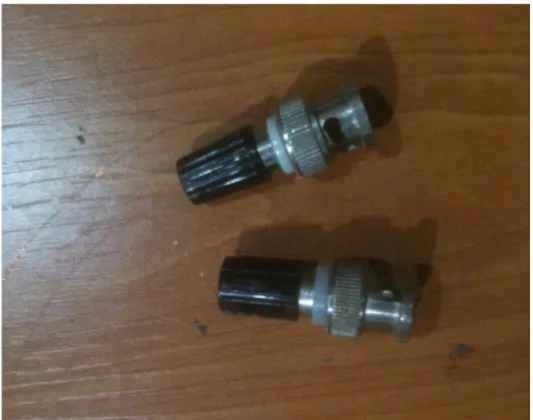
To keep the incoming flux as minimum as possible, the wires are twisted (see section 2.1.1). Some wires can only be twisted by hand but for long wires there is a little trick. Start by cutting off a wire twice as long. Put equal weights on both ends of the wire.
Figure 3.2:The weights used for the ends
weight should just be above the other. Twist the top part of the wire and the weights will start to follow in a circular motion. After some twists, the weights have gained a momentum and the wire will start twisting on its own. The reason for having the weights not on the same height is that they will keep spinning longer in the end.
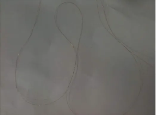
When the wires are done spinning, glue can be applied to the whole wire to make it stronger. Do not take the wire off immediately, try to keep it as straight as possible. When the tension on the wire releases, curls will sometimes occur like the figure below.
Figure 3.3:The telephone curl effect on a wire.
3.2
The Elliptical Coils
3.2.1
Winding the Coils
In the circuit we see two opposite placed coils which are connected in se-rie. The blueprint for one holder of the coils is shown below in figure 3.4. These holders are made of plastic.
Figure 3.4:A holder
The windings are made by placing the holder in a rotating device as seen in figure 3.5 which can be spun by a motor or by hand. Spinning by hand gives more control but requires more effort. Winding the coil becomes easier when a microscope is used.
Figure 3.5: The holder in the rotating device. One end of the wire is taped to the rotator and the other is held with tension from the wire coil.
The coil where the niobium-titanium wire comes from should be able to freely rotate without much resistance and should be mounted in a place where the wire to the holder does not become obstructed.
should be twisted together. The process for the second coil is exactly the same.
One coil has the pick-up loop while the other gets the excitation loop. Winding the excitation loop is just a case of fitting a niobium-titanium wire around the top and glueing, leaving ends of 10 cm. The pick-up loop requires more work: it is made of more fragile 50µm niobium wire
and winded around the smaller loop around the cave. The excitation loop wires needs to be twisted with itself and the pick-up loop wire also with itself.
Finally, a layer of phenol is applied to keep the coil really firm.
If a small mistake occurs, the glue can be dissolved using acetone. The remaining glue could be scraped off with the needle. If there is still too much glue, the holder can be placed in a beaker with acetone and shaken thoroughly.
3.2.2
Assembling the Coils
The two coils are assembled in a special case as seen below in figure 3.6. We can neglect the green part. It is necessary that the long side of the ellipses are placed along the same direction without any deviation. The grooves where the pick-up loop comes out can be seen from the outside. These grooves both run out at the long side of the coils and can therefore be used to calibrate the ellipses. The grooves should be on top of each other.
In figure 3.6 we can see a circular cut out part at the right side of the as-sembly. A similar cut can be seen on the other side on the right of the assembly. The niobium-titanium wires should run along one cut and the niobium pick-up wire along the other cut.
The whole assembly is placed in a niobium container with the wires run-ning out as seen in figure 3.7.
Figure 3.7:The metal container with the wires running out marked ”Boven” and ”Onder”.
3.3
The Big Coil
3.3.1
The Machine
A machine (figure 3.8) is used for winding the big coil. This is because the big coil requires a lot more windings: around 10.000. This was calculated with equation 3.3.
Figure 3.8
The machine consists of:
A wire coil
The big coil
The big coil is the coil in the middle of the figure where the light shines upon and is made of plastic.
The dimensions of the big coil are:
length = 18mm, inner radius = 4.5mm and the outer radius = 11mm. The big coil also has a hole for the shortcut to run through which has a radius of 1.5mm. The dimensions are chosen such that with wire of a diameter of 120µm,n=8125 can be reached.
A leading wheel
The wire from the wire coil runs through a leading wheel, which goes back and forth to spin the wire evenly over the big coil. The leading wheel can be seen just above the big coil. The back and forth motion of the leading wheel can be turned off on the machine. The velocity at which is goes is determined by setting the diameter of the wire. The boundaries at which it goes back and forth is limited by adjustable locks on each side.
A microscope
The microscope can be seen on the left side and is directed at the big coil.
A counter
The counter is on the left side of the green machine and gives the count in numbers. Be sure to set the counter to zero when you start with wiring. In this case, the counter gives one count every two windings so the value must be doubled to get the true number of windings.
A pedal
The pedal is on the ground and turns on the rotating device. The velocity depends on how far the pedal is pushed in. The maximum velocity is adjustable on the machine.
3.3.2
Making the Big Coil
Locking something in the rotating device works the same as locking a drill bit into a drill machine. So a drill bit has to be found which can fit in the hole of the big coil. To make it tight, we can use teflon tape around the drill bit.
cases.
Try to keep everything as tight as possible, especially the sides. After a while this becomes impossible but how tighter it is in the beginning, how easier the rest of the winding becomes.
Figure 3.9:A picture of the big coil taken to the microscope, hence the black circle on the bottom. Note how tightly the wire is stuck together.
A way to keep it tight is to let the leading wheel run a bit behind the posi-tion of the wire on the coil and have some tension on the wire. The tension causes the wire to fall tightly to the side of the winding before. Glue can applied every once in a while to keep it in place, but the downside in this case is that the wire becomes harder to use when everything needs to be done again.
Equation 3.3 rewritten gives:
I = 2Bcritr
µ0n ≈0.723A. (3.4)
This is quite a high current, and can result in the experiment heating up. Experiments have to be made to make sure that this does not happen.
A layer of Stycast is put over the wires to make it stable. The Stycast needs a day to dry at room temperature. This process can be accelerated using a blow-dryer.
The ending of both wires should also be twisted and put in a teflon sock. This sock should then be hold on one side of the big coil with a thread. Let the big coil stand on the other side and apply a layer of Stycast over the side with the teflon sock. Be careful that no Stycast comes into the hole where the niobium wire goes through, we can close this hole off with a cotton bud. The same procedure is done on the other side.
Put the coil back on the machine and let it run at a low velocity with a big layer of Stycast all around it. This amount of Stycast is necessary to make sure the coil does not explode when it reaches a temperature of 4 Kelvin.
The big coil now looks like a black barrel with a clear hole in the middle and a teflon sock with wires running out of it.
3.4
The Lead Particles
The lead particles are made by scraping off a little bit from a bigger block of lead. Gloves can be worn to protect against lead dust on the hands. The scraped off lead is put on a thick piece of metal. This metal will become really hot so it must be placed well. With the help of a Dremel burner we heated up the lead scrape until it starts to melt a bit. The burner should not heat the scrape too long, there must be small pauses between every heating.
Figure 3.11:The Dremel burner
The scrape melts faster when it is occasionally turned around. Eventually the scrape will turn into a round ball.
In this experiment five balls are made: 2 small sized and 3 large sized as can be seen in figure 3.12.
The wire running underneath the balls is a 50µm niobium wire. The
di-ameter, and therefore the mass can be approximated with the picture. We look at how many times the wire fit in the balls by zooming in the picture.
The volume is calculated byV = 43πr3= 16πd3.
The mass is calculated bym=ρV whereρ=11.34 g/cm3.
n times width wire d (cm) V (cm3) m (g)
small balls 4.5 2.25·10−2 5.96·10−6 6.76·10−5
large balls 6 3.00·10−2 1.41·10−5 1.60·10−4
The balls are given different shapes with the help of pliers until they look like the figure below.
0.7mm Figure 3.13:The balls after giving dents
From left to right they got the shape by:
3.5
Preparing the Dipstick
The dipstick is a long stick with a plate on the end where the experiment will be mounted. The stick goes in a barrel with helium-4 where it will reach a temperature of 4 Kelvin, therefore below the critical temperature of niobium-titanium, niobium and lead.
We begin by making two cables which send data back and forth through the stick. One cable is for the SQUID and connects to a 14 pins female LEMO on the top, the other cable ensures data flow from the coils and connects to a 24 pins Fischer.
Below we see the 24-pins Fischer with the corresponding data numbers. We want to solder 10 niobium-titanium wires to the numbers 1 to 10 but it becomes easier if we prepare the wires first.
One wire with a length a bit longer than double the dipstick is twisted with the method used in section 3.1.3. The wire is cut in the middle so it becomes two wires. Enter these two wires through a teflon sock. Any bends will make it harder for the wire to be entered through the sock. Another way to get them through is by soldering a stronger wire to the two wires and running this wire first through the sock. The two wires can then be pulled through when the stronger wire is starting to exit.
We end with five teflon pairs. The pairs are labeled 1 to 5 with the label close to one end.
Solder the wires with the label ’1’ to the pockets 1 and 2, label ’2’ to pockets 3 and 4 etc. The labels need to be close to the other end of the wires.
We make sure they conduct by measuring the resistance. The ten wires are run through a metal coating to ensure a Faraday cage. The coating has the same length as the tube of the dipstick, but because the wires are longer, the wires will stick out with the labels on this end. To ensure stability, we put a layer of Stycast around the coating where it makes contact with the Fischer. We put silver coating around this to close the Faraday cage.
The second cable can be bought to fit from the SQUID to a 14-pins LEMO.
Run these two cables first through the dipstick so they end at the plate. The labels need to be visible here.
We then mount the elliptical coils on the plate with a special design with screws the tube to the plate.
Figure 3.16: The wires are not in this picture because we did it the other way around and ended up taking apart everything because one cable did not fit through.
The wire which runs from the pickup coil in between the elliptical coils to the SQUID needs to be put in a teflon sock first, and then through a lead tube which fits tightly around the sock. To cut the lead tube, be sure to have a thicker wire running through so the pressure will not close the ends together.
We can put the squid on the plate to see where it fits.
The big coil is put on this plate next to the SQUID and held using teflon tape.
Everything is spot welded together using niobium as the connector be-tween the wires and Kapton tape around to ensure everything stays in place. The labels correspond to the numbers in the scheme (figure3.1).
The wire which goes through the big coil is spot welded as seen in the circuit (figure 3.1). This wire is bend in the middle and twisted. After this it is then put through the big coil. This way we can easily remove the wire if there occur any problems.
The SQUID cable is fit into the SQUID. Layers of teflon tape are wound up around the plate until everything stays tightly together.
Figure 3.18:The experiment taped together with teflon tape. This way everything stays tight together.
Figure 3.19:The final product of the dipstick.
Chapter
4
Numerical Calculations and
Predictions
4.1
The Magnetic Field
The codes are written in Mathematica. They are meant for the elliptical coils, but can be used for the circular coils when a and bare made equal. The equations for the magnetic field are exactly the same as 2.22, 2.23 and 2.24.
The constants we use are close to the correct constants of the experiment.
mu0 = 4*Pi*10^(-7) (*The magnetic permeability of air*); i = 0.25 (*The current in Ampere*);
a = 2 (*Distance between origin and ellipse along x in mm*); b = 1 (*Distance between origin and ellipse along y in mm*);
d = 1 (*Distance between the origin of the ellipse and z=0 in mm*); n = 255 (*Number of windings*);
The reason why millimeters are used instead of the SI-Unit ”meter” is be-cause Mathematica gives much better streamplots when higher numbers are used.
calculates everything numerically, and is therefore quicker.
bx[x_?NumericQ, y_?NumericQ, z_?NumericQ] := mu0*i*b*n/(4*Pi)*
NIntegrate[((z +
d)/(x^2 + y^2 + (z + d)^2 + a^2*Cos[t]^2 + b^2*Sin[t]^2 -2*a*x*Cos[t] - 2*b*y*Sin[t])^(3/2) (z
-d)/(x^2 + y^2 + (z - d)^2 + a^2*Cos[t]^2 + b^2*Sin[t]^2 -2*a*x*Cos[t] - 2*b*y*Sin[t])^(3/2)) Cos[t], {t, 0, 2 Pi}]
(*The x component of the magnetic field*)
by[x_?NumericQ, y_?NumericQ, z_?NumericQ] := mu0*i*b*n/(4*Pi)*
NIntegrate[((z +
d)/(x^2 + y^2 + (z + d)^2 + a^2*Cos[t]^2 + b^2*Sin[t]^2 -2*a*x*Cos[t] - 2*b*y*Sin[t])^(3/2) (z
-d)/(x^2 + y^2 + (z - d)^2 + a^2*Cos[t]^2 + b^2*Sin[t]^2 -2*a*x*Cos[t] - 2*b*y*Sin[t])^(3/2)) Sin[t], {t, 0, 2 Pi}]
(*The y component of the magnetic field*)
bz[x_?NumericQ, y_?NumericQ, z_?NumericQ] := mu0*i*n/(4*Pi)*
NIntegrate[(1/(x^2 + y^2 + (z + d)^2 + a^2*Cos[t]^2 +
b^2*Sin[t]^2
-2*a*x*Cos[t] - 2*b*y*Sin[t])^(3/2)
-1/(x^2 + y^2 + (z - d)^2 + a^2*Cos[t]^2 + b^2*Sin[t]^2 -2*a*x*Cos[t] - 2*b*y*Sin[t])^(3/2)) (a*b - a*y*Sin[t] -b*x*Cos[t]), {t, 0, 2 Pi}] (*The z component of the magnetic
It would be nice to look at the symmetric properties of the elliptical fields. We can therefore plot the field in a y=0 and x=0 plane.
StreamPlot[{bx[x, 0, z], bz[x, 0, z]}, {x, -3, 3}, {z, -3, 3}, StreamColorFunction -> "Rainbow",
PlotLabel -> "Magnetic Field Lines",
FrameLabel -> {"x(mm),", "z(mm)"},
PlotLegends ->
BarLegend[Automatic,
LegendLabel -> "Magnetic Field Intensity (kT)"]] (*Streamplot in y=0 plane*)
StreamPlot[{by[0, y, z], bz[0, y, z]}, {y, -3, 3}, {z, -3, 3}, StreamColorFunction -> "Rainbow",
PlotLabel -> "Magnetic Field Lines",
FrameLabel -> {"y(mm)", "z(mm)"},
PlotLegends ->
BarLegend[Automatic,
LegendLabel -> "Magnetic Field Intensity (kT)"]] (*Streamplot in x=0 plane*)
This code gives the figures 4.1(a) and 4.1(b).
(a)Magnetic field lines in the y=0 plane
(b)Magnetic field lines in the x=0 plane
We can clearly see the radii1of the current loop. In the y=0 plane the upper current loop shows a radius of 2 and in the x=0 plane a radius of 1. Because we work in millimeters, the unit of the magnetic field is in kT.
The graphs show some problems: anti-symmetry around (0,0) in both fig-ures 4.1(a) and 4.1(b). This is probably because of the way how Mathemat-ica calculates the streams. The way the upper half of the function interacts with the lower half around (0,0) can force Mathematica to take arbitrary values. We can look if this is true by plotting with different limits.
Figure 4.2:The limits are changed: x ={-1, 1}and z ={-2,0}
We see that the function is now symmetric and the anti-symmetry is caused by Mathematica.
1The meaning of the radius of an ellipse can differ. In this case we mean the distance
To see the elliptical field in the z=0 plane clearly, we can make a vectorplot.
VectorPlot[{bx[x, y, 0], by[x, y, 0]}, {x, -3, 3}, {y, -3, 3}, VectorColorFunction -> "Rainbow",
PlotLabel -> "Magnetic Field Vectors",
FrameLabel -> {"x(mm)", "y(mm)"},
PlotLegends ->
BarLegend[Automatic, LegendLabel -> "Field Intensity (kT)"]
(*Vector plot in the z=0 plane*)]
With its corresponding figure:
Figure 4.3:The largest vectors are close to the shape of the elliptical coils
We see that in the middle it has no magnetic field. This is a property of the anti-Helmholtz configuration. The potential is lowest at this point so the particles tend to stay as close as possible to this point.
and small vectors on the side of the graph. The big difference between values of the vectors causes the 3D plot to act chaotically.
Also, the experiment takes place around the origin. So for the 3D plot it is better to take values limits close to the origin.
VectorPlot3D[{bx[x, y, z], by[x, y, z], bz[x, y, z]}, {x, -0.8, 0.8}, {y, -0.8, 0.8}, {z, -0.8, 0.8},
VectorColorFunction -> "BlueGreenYellow",
PlotLabel -> "Magnetic Field Vectors",
AxesLabel -> {"x(mm)", "y(mm)", "z(mm)"},
PlotLegends ->
BarLegend[Automatic, LegendLabel -> "Field Intensity (kT)"]] (*3D Vector plot*)
Figure 4.4:A three dimensional plot of the field close to its zero potential.
4.2
Approximating the Magnetic Field
The constants are converted to SI-units so the magnetic field is calculated in Tesla. This is convenient because the magnetic field is going to be nu-merically approximated.
mu0 = 4*Pi*10^(-7) (*The magnetic permeability of air*); i = 0.25 (*The current in Ampere*);
a = 2*10^-3 (*Distance between origin and ellipse along x in m*); b = 10^-3 (*Distance between origin and ellipse along y in m*); d = 10^-3 (*Distance between the origin of the ellipse and z=0 in
m*);
n = 255 (*Number of windings*);
ds = 10^-5 (*The infinitesimal length for the derivatives*);
The code for the plots of the magnetic fields is shown below.
Plot[bx[x, 0, 0], {x, -10^-3, 10^-3},
PlotLabel -> "Value Magnetic Field", AxesLabel -> {"x(m)",
"Bx(T)"}] (*The x-component of the magnetic field*)
Plot[by[0, y, 0], {y, -10^-3, 10^-3},
PlotLabel -> "Value Magnetic Field", AxesLabel -> {"y(m)",
"By(T)"}] (*The y-component of the magnetic field*)
Plot[bz[0, 0, z], {z, -10^-3, 10^-3},
PlotLabel -> "Value Magnetic Field", AxesLabel -> {"z(m)",
"Bz(T)"}] (*The z-component of the magnetic field*)
(a) (b)
(c)
Figure 4.5: The magnetic fields with the same limits as the sphere in which the Zeppelin can move.
At the edges we can see the slope decreasing which indicates a third de-gree polynomial. However, for the following calculations we assume that the particle stays close to the origin and can therefore be approximated with a first degree polynomial as shown in equation 2.33).
These constants are found by taking the derivative of the function at their origins. The derivative is calculated by:
a1 := (bx[ds, 0, 0] - bx[-ds, 0, 0])/(2* ds) (*The derivative of bx to x*)
b1 := (by[0, ds, 0] - by[0, -ds, 0])/(2* ds) (*The derivative of by to y*)
c1 := (bz[0, 0, ds] - bz[0, 0, -ds])/(2* ds) (*The derivative of bz to z*)
And gives the following slopes:
In[228]:= {a1, b1, c1}
Out[228]= {7.90315, 24.6639, -32.567}
The resulting magnetic field will then be:
~B(x,y,z) =7.90xxˆ+24.66yyˆ−32.567zzˆ. (4.1)
Remarkable is how the absolute of the slope in the z direction is the sum of the other two slopes. This is explained by one of the Maxwell’s equations, namely:
~
∇ ·~B =0 (4.2)
Which gives:
∂
∂xa1x+ ∂
∂yb1y+ ∂
4.3
Resonance Frequencies
4.3.1
Translational Frequencies
The force components of a superconducting sphere is given by the code below. The forces are calculated and given by equation 2.34.
forcex[x_] := -(8*Pi r^3)/(3*mu0)*a1^2* x (*Force in the x direction*)
forcey[y_] := -(8*Pi r^3)/(3*mu0)*b1^2* y (*Force in the y direction*)
forcez[z_] := -(8*Pi r^3)/(3*mu0)*c1^2* z (*Force in the z direction*)
The spring constants are given by:
kx := (8*Pi*r^3)/(3*mu0)*a1^2
(*Spring constant in the x direction*)
ky := (8*Pi*r^3)/(3*mu0)*b1^2
(*Spring constant in the y direction*)
kz := (8*Pi*r^3)/(3*mu0)*c1^2
(*Spring constant in the z direction*)
The constants given above will give the following spring constants:
In[156]:= {kx, ky, kz}
Out[156]= {0.00124919, 0.0121662, 0.0212122}
As expected, the spring constants become higher in the orderkx <ky <kz.
We get the frequency out of the spring constant by:
f = 1
2π
r
k
m (4.4)
With the corresponding code:
fx := 1/(2*Pi)*Sqrt[kx/m] (*frequency in the x direction*)
fy := 1/(2*Pi)*Sqrt[ky/m] (*frequency in the y direction*)
fz := 1/(2*Pi)*Sqrt[kz/m] (*frequency in the z direction*)
And at last, the resulting frequencies are:
In[203]:= {fx, fy, fz}
Out[203]= {10.2701, 32.0506, 42.3206}
We also see here that the frequency in the z direction is the sum of the other two frequencies. This is explained by the fact that the slope of the magnetic field in the z direction is the sum of the other two slopes as seen in 4.3.
We take the z frequency from equation 2.35 and rewrite it:
fz =
|c| 2π
s
2
µ0ρ =
|a+b| 2π
s
2
µ0ρ =
|a| 2π
s
2
µ0ρ +
|b| 2π
s
2
µ0ρ = fx+fy (4.5)
4.3.2
Rotational Frequencies
Unfortunately, we have not been able to find the rotational frequencies. Nonetheless we can make assumptions on how to find these.
We can calculate the magnetic dipole moment by using the equation:
~F =∇(~B·m~). (4.6)
The magnetic dipole moment was also calculated this way in the thesis of T. De Jong and D. Kok [12], however there will only be a magnetic dipole moment when it is off-axis. Further calculations with these off-axis results will be difficult.
The next step is to calculate the torque exerted on the particle:
~τ =~m×~B. (4.7)
The work the torque does is given by the integral:
W =
Z
θ2θ1
τdθ, (4.8)
which is equal to the energy:
ER = 1
2Iω
2
. (4.9)
Chapter
5
Results and Discussion
5.1
The Lead Zeppelin Experiment
The whole dipstick for the new asymmetrical Lead Zeppelin is now fin-ished. All the components are made to fit in the dipstick. The dipstick is airtight and gives no problems when sucking vacuum.
A lot of time was put in the big coil. The wire kept breaking and glue was accumulating on the wire which made it harder to wind. Optimal would be to have around 10.000 windings, but 6828 should in theory be enough.
Furthermore, five lead balls have been made for following experiments. These should be enough because they all have different properties.
The wires running through the big coil and elliptical coils have been mea-sured and show a resistance in the right range. The resistance of the other wires have also been tested and they are all conducting with sensible re-sistances.
An effort has been made to make the components as invulnerable as pos-sible. All the wires are put in teflon socks. The wires are then bounded together so no wire gets hooked behind something.
The Lead Zeppelin has three Faraday cages to reduce the EM noise.
The dipstick was carefully placed in a barrel of helium-4. The
manome-ter showed a pressure of 10−3 millibar. The SQUID and voltage meter
millibar. This did not make any difference.
The results on the computer showed that the voltage meter measures a charge build-up when the switch was still turned off. This means that the current flows through the elliptical coils instead of the shortcut. We have replaced the shortcut with a new niobium wire but the results stay the same. It could be the case that the shortcut is not cold enough to super-conduct, but the reason has not been found.
5.2
Numerical Results
The magnetic field of the elliptical coils with I = 0.25A is approximated by:
~B(x,y,z) =7.90xxˆ+24.66yyˆ−32.567zzˆ. (5.1)
With resulting frequencies: fx = 10.2701 Hz, fy = 32.0506 Hz and fz =
42.3206 Hz.
When we calculate the field for circular coils with a radius of√ab, so the areas stay the same, we get:
~B(x,y,z) =15.42xxˆ+15.42yyˆ−30.83zzˆ. (5.2)
With resulting frequencies: fx= 20.035 Hz, fy= 20.035 Hz, fz= 40.0686 Hz.
For the ellipse, the field lines get squeezed in the y direction, and therefore loosened up in the x direction when we assume that the fluxes are the same. This explains the lower slope in the x direction, and higher slope in the y direction. This can also be mathematically verified by replacinga
andbwith√abin equations 2.22, 2.23 and 2.24.
We see that we can distinguish the x and y frequencies even better by making the shape more elliptical, or in other words: increase the ratio ab, whereaandbare the elliptical properties.
By doubling the current to 0.5 Amp`ere, we get the following frequencies for elliptical coils: fx = 20.5402 Hz, fy = 64.1012 Hz and fz = 84.6413 Hz.
We see that the frequencies get doubled, so the difference between fxand
fy should also be twice as much. This property can be used for better
5.3
Fourier Spectrum of the Spherical Lead
Zep-pelin with Circular Coils
The Lead Zeppelin with elliptical coils has no results yet. Nonetheless, we could still look at the results of the circular Lead Zeppelin with a asym-metrical lead particle.
The Fourier Spectrum of the Lead Zeppelin with circular coils is given below.
Figure 5.1: Frequency spectrum of an aspherical Zeppelin in between circular coils at 0.35 A right after a kick to the Dewar. We see many non-linearities from mixing and doubling frequencies.
With the 6 frequencies marked:
We find the 6 frequencies by choosing sets. We choose fundamental fre-quencies as seen in the ”calculated” row in figure 5.3. These frefre-quencies show many similarities but other sets can always be chosen as fundamen-tal frequencies.
Figure 5.3:Part of the Excel file which includes data of the peaks
The yellow boxes are the frequencies which are in their error margins. The orange boxes show those outside their error margins. The red boxes are nowhere to be found. We can apply these peaks to the frequency spectrum and get figure 5.2 as result.
The translation frequencies in the x and y direction should be close to-gether, in theory they should be at the same frequency. Therefore, it is logical to assume B and C are the translational x and y frequencies.
therefore we assume D is the translational z frequency. However, this as-sumption is not mathematically verified.
Since we do not have a mathematical model for the rotational frequencies, we can only find these frequencies by reasoning. The only way to have a translational frequency around the z-axis, is to have inhomogeneities in the field. This creates a low frequency since these inhomogeneities are far lower than the change in magnetic field in other directions. Therefore, we assume that A is the rotational frequency around the z-axis.
This leaves us only with E and F for the other two rotational frequencies. The Zeppelin has a long and a short side, and wants to stay in one posi-tion since the potential must be the lowest in this posiposi-tion. Let us assume the longer side lies along the x direction. The rotation of the longer side, around the y-axis, has a bigger moment of inertia. This frequency must be therefore lower than the rotation frequency over the shorter side, around the x-axis. Peak E should be the rotation frequency of the longer side and F of the shorter side.
Chapter
6
Conclusions
All the components are built, only the switch needs to be made to work. If this is done, one could most likely start to measure immediately. After this, we can look if the theoretical and numerical predictions are correct. The peak of the rotational frequency around the z-axis must shift to a higher frequency, the other rotational frequencies are now more defined by the elliptical properties and the translational frequencies should be better dis-tinguishable.
Chapter
7
Follow up Experiments and
Improvements
Since this experiment has just been built, it has a lot of room for follow up experiments and improvements. The most important follow up exper-iments are:
• Getting the Lead Zeppelin to work properly.
It is not clear if there are more problems with this new Lead Zeppelin project because it has not yet been put to the test. Maybe also other parts need replacement or optimization.
• Calculating the rotational frequencies.
The rotational frequencies have not yet been calculated and require a bit more work than the translational frequencies.
• Comparing the results to the symmetrical Lead Zeppelin.
In theory only differences between the frequencies should be shown. In reality there could be more differences and set backs.
• Finding the corresponding frequencies.
Some improvements could be made like:
• Finding equations for the distributed loops.
The magnetic field of the coils has been calculated by assuming that the loops overlap at the same position. A better calculation takes care of this by distributing the loops over the length of the coil.
• Finding the Taylor expansion of~B of the elliptical coils.
The slopes of the magnetic fields should be a function of the vari-ables used. The numerical approach is taken in this project, but a mathematical approach can also be done.
• Distinguish the x and y frequencies better.
This can theoretically be done by increasing the current or making more asymmetrical coils.
• Finding the Q factor.
The symmetrical Lead Zeppelin uses different material for the as-sembly of the coils and different Faraday cages. This can result in a different Q factor.
• Putting the coils in a vibration-reducing cage.
Chapter
8
Acknowledgements
I would like to thank Tjerk Oosterkamp for granting me the opportunity to do this experiment. I think this was one of the few experiments this year which really sounded interesting to me. It has a good balance between the mathematics, hand crafting and computation. Every day had another goal (except the long period when I had to wind the big coil and it kept breaking) which really gave this experiment an adventurous feeling.
Also I would like to thank Bob for helping me out a lot in the beginning. The instructions for the experiment were always on point and you steered me every time in the right direction. That became clear when I tried to do the experiment alone and immediately cooked a barrel of helium.
Next, I want to thank everyone who provided me with information about this experiment. Including Martin de Wit, Tobias de Jong and David Kok. You did a great job writing all the necessary parts down.
I am grateful for everyone in the Interface Physics group for everything: from getting good coffee beans to helping me find stuff in the lab.
Outside the group I am indebted to the people of the FMD, especially Gert Koning, who literally made the whole experiment. There was al-ways someone in the FMD who could help me with the material of the experiment.
Netherlands for granting people the opportunity to get such good educa-tion. Tesla for the steady current flow through the lab. Bruch, Dvoˇr´ak, Ray Charles and The Benny Goodman Orchestra for getting me through the long computation times. You have all been very lovely.
I am closing another chapter of my life and I am grateful that I am still motivated to learn more, even after all these years of school. I have learnt that good motivation comes from the small things like seeing your friends each day or listening to a great piece of music on the way home. I had a great time here at Leiden and hopefully see you all again.
[1] C. L. Degenet al., “Nanoscale magnetic resonance imaging,” PNAS, 2009.
[2] O. Romero-Isartet al., “Quantum magnetomechanics with levitating superconducting microsphere,”Phys. Rev. Lett. 109, 147205 (2012). [3] “Meissner effect.” [Online]. Available: https://en.wikipedia.org/
wiki/Meissner effect
[4] M. de Wit, “The lead zeppelin project,” 2012.
[5] D. J. Griffiths,Introduction to electrodynamics, 4th ed. Pearson, 2013.
[6] “Superconductors.” [Online]. Available: http://www.
superconductors.org/INdex.htm
[7] “High-temperature superconductivity,” Helsinki University of Tech-nology, Tech. Rep., November 2008.
[8] M. Peiniger and H. Piel, “A superconducting nb3sn coated multicell accelerating cavity,”IEEE Transactions on Nuclear Science, vol. 32, no. 5, 1985.
[9] R. Fl ¨ukiger et al., Nb-Ti. 21b2: Nb-H - Nb-Zr, Nd - Np (The Landolt-B¨ornstein Database ed.). SpringerMaterials, 1994.
[11] E. Diez-Jimenez, J.-L. Perez-Diaz, and J. C. Garcia-Prada, “Local model for magnet–superconductor mechanical interaction: Experi-mental verification,”Journal of Applied Physics, 2011.