Sharif University of Technology
Scientia IranicaTransactions B: Mechanical Engineering http://scientiairanica.sharif.edu
Research Note
A comparison of some methods for structural damage
detection
K. Rezvani
a, N.M.M. Maia
b, and M.H. Sabour
a;a. Department of Aerospce Engineering, Faculty of New Sciences & Technologies, University of Tehran, North Kargar, Tehran, Iran. Zip Code: 1439957131.
b. Department of Instituto Superior Tecnico, Universidade de Lisboa, Av. Rovisco Pais Lisboa, Portugal. Zip Code: 1049-001. Received 15 November 2016; received in revised form 14 February 2017; accepted 20 May 2017
KEYWORDS Structural health monitoring; Damage detection; FRF curvatures; Modal testing; Damage indicator.
Abstract. In principal, a proper analysis of the dynamic response of a structure can provide general indicators of its operational conditions. When the dynamic response changes due to variations of the physical properties of a structure, then one may conclude that some kind of damage has occurred. This paper presents an investigation of the robustness and comparison of four simple methodologies to both identify and quantify the damages in structures, based on the use of Frequency Response Functions (FRF) signals, Principal Component Analysis technique (PCA), and transmissibility. A steel beam with constant rectangular cross-section is used to compare the proposed approaches. At rst, nine damaged scenarios are created, for each of which numerical examples are discussed; a database of FRFs is measured using modal testing. Then, PCA theory is applied to the FRF matrix, and global damage detection and quantication indices are dened using the rst three principal components; Hotelling's T-squared distribution is also applied, and two other indicators, transmissibility damage indicator and weighted damage indicator, are computed for the assessment of damage using transmissibility. The reported examples show that all proposed methods are able to detect and quantify damages at the initial stage. © 2018 Sharif University of Technology. All rights reserved.
1. Introduction
Nowadays, the interest in the ability to monitor a struc-ture and identify damages at the earliest possible stage is pervasive throughout aerospace structures, bridges, civil infrastructures, and mechanical engineering sys-tems. Detection and localization of damage allows one to reduce maintenance costs and ensure safety [1-3]. Several non-destructive inspection methods (NDE) for the evaluation of the health condition of a structure
*. Corresponding author:
E-mail addresses: [email protected], and [email protected] (K. Rezvani);
[email protected] (N.M.M. Maia); and [email protected] (M.H. Sabour).
doi: 10.24200/sci.2017.4494
are currently available such as acoustic or ultrasonic methods, magnet eld methods, radiographs, eddy-current methods or thermal eld methods, etc. Un-fortunately, these experimental techniques may be dif-cult, costly and unreliable, because damage location must be known in advance, or it is often necessary to expose the structural elements and the equipment to the inspector for detecting damage, with relevant accessibility problems. This is the reason for which alternative approaches in recent decades are mainly based on the changes of the vibration characteristics or the responses of the structures caused by a structural damage; consequently, such approaches have received considerable attention in the literature [4-7]. For example, some authors have localized some damages by comparing identied mode shapes or their second-order derivatives [8] in varying levels of damage. Sampaio
et al. [9] extended the method proposed in [8] with measured FRFs. Failing to consider just the FRFs in the low-frequency range, Friswell [10] presented an overview of the usage of inverse methods in damage detection and location by measured vibration data. Liu et al. [11] used the imaginary part of FRF shapes and normalized FRF shapes to achieve damage local-ization. Their method was illustrated by a numerical example of a cantilever beam. Natural frequency sensitivity was also used extensively for the purposes of damage localization. Ray and Tian [12] discussed the sensitivity of natural frequencies with respect to the location of local damage. In that study, damage localization has involved the consideration of changes in the mode shapes. Zhou et al. [13] and Zhou and Perera [14] used power spectral density transmissibility to detect damages using modal assurance criterion and articial neural networks, respectively; Zhao et al. [15] discussed damage detection and localization using the transmissibility-based nonlinear feature analytically.
The fundamental idea of the vibration methods for damage detection is that modal parameters (natural frequencies, mode shapes, and modal damping) are functions of the physical properties of the structure (mass, damping, and stiness). Therefore, changes in the physical properties will cause detectable changes in the modal properties. Therefore, this process involves the observation of a structure/system along the time using periodical measurements. In other words, most vibration-based damage detection methods can be con-sidered as a form of the pattern recognition problem. As they look for the discrimination between two or more signal categories, e.g. before and after a structure is damaged or for dierences in the damage levels or locations. In this situation, it is common to deal with a large variety of complex systems in which the number of variables to be measured can be unwieldy and even sometimes deceptive, because the implicit relationships can often be quite simple.
The main problem in applying this approach is the very small magnitude variation of dynamic response due to structural damage related to the local variation of stiness, mass, and damping. Aiming to overcome these drawbacks, more explicit and capable methods are needed to detect the presence of damage even in the case of small variation of the dynamic response, in addition to the need for a method to reduce the requested amount of data. Several data reduction techniques are available for this purpose. The potential advantages of this kind of approaches can be summa-rized as follows:
- They represent indirect diagnostic methodologies for damage detection based on the recognition that changes in the dynamic characteristics of the struc-ture are related to various damage states;
- They do not require direct exposure of structural elements;
- They inspect the whole structure in one dynamic test;
- They favor a reduction in schedule and cost. In this paper, damage detection in a steel beam is carried out using four new dierent methods by the vibration response data directly measured along a structure during modal testing. Those methods are able to identify and quantify the damage us-ing transmissibility techniques, Hotellus-ing's T-squared distribution, and the principal components of FRF matrices.
The paper is organized in six sections. Section 2 gives a brief description of damage identication meth-ods. Section 3 introduces the beam structure used for the validation of damaged scenarios investigated during modal testing. Section 4 describes the FE model of the considered beam and includes the application of adopted damage detection methods to the simulated damage scenarios. Section 5 presents experimental modal testing and related results. Finally, Section 6 concludes the paper.
2. Brief theoretical description of the developed methods
2.1. Principal component analysis
Principal Components Analysis (PCA) is a standard tool to identify patterns in data and represent the data in a manner that highlights their similarities and dissimilarities. In other words, PCA is an attractive numerical procedure for analyzing the basis of the variation present in a multi-dimensional dataset and identifying the most meaningful basis to re-express a dataset. PCA is called one of the most valuable results derived from applying linear algebra developed by Jollie [16] and Bishop [17]. It can be viewed as a statistical technique capable of realizing a dimension-ality reduction, based on a transformation from the original set of variables into a new set of uncorrelated variables, i.e. the Principal Components (PC). Using an orthogonal projection, the original set of variables in an N-dimensional space is transformed into a new set of uncorrelated variables, the Principal Components, in a P -dimensional space, such that P < N. It is assumed that all FRF data are equally important in describing the underlying features of the baseline signals, and the standard \auto scaling" procedure is performed for pre-preprocessing. By \auto scaling", each column of the FRF matrix is arranged to have a zero mean (by subtracting the mean value of each column) and to have a unit variance (by dividing each column by its standard deviation). The procedure is described below. Using all available FRF data of the intact structure,
FRF matrix H has N rows of FRFs (N observations from dierent sensors), each with M frequency points. Each element is denoted by Hij(!). The mean response
( Hi) and standard deviation (Si) of the ith row can be
dened as follows:
Hi= M1 M
X
j=1
Hij(!); (1)
Si2=M1 M
X
j=1
(Hij(!) Hi)2: (2)
It is possible now to calculate response variation ma-trix, ~H(!)NM, where a typical element of the Hij(!)
FRF matrix can be replaced by: ~
Hij(!) = Hij(!)
Hi
SipM : (3)
Sample covariance matrix, C, can be dened as fol-lows [18,19]:
C = ~H(!)NMH(!)~ TMN; (4) where ~H(!)T is the matrix transpose measurement, C
is a NN matrix whose diagonal terms are the variance of N variables, and non-diagonal terms represent the covariance between variables.
By denition, the Principal Components (PCs) are the eigenvalues and associated eigenvectors (prin-cipal loadings) of the covariance matrix:
C i= i i: (5)
The rst principal component, i.e. the highest eigen-value and its associated eigenvector, represents the amount and direction of the maximum variability in the original data. The next one, which is orthogonal to the rst component, represents the next most signicant contribution from the original data, and so on. Finally, to perform PCA is simple in practice through the basic steps [20]:
1 Organize the dataset as a M N matrix, where M is the observations from dierent sensors and N is the number of frequency lines;
2 Normalize the data to have zero mean and unity variance;
3 Calculate the eigenvectors and eigenvalues of the correlation (covariance) matrix;
4 Select the rst eigenvectors as the principal compo-nents;
5 Transform the original data by means of the princi-pal components (projection).
Concerning the damage detection, rstly, Global Dam-age Index (GDI) can be introduced as a function of the rst principal components (often the rst three ones) as follows [20]:
GDI3P C =
v u u tX3
i=1
(P Ci)2; (6)
where P Ci represents the relative variation between
the ith principal component related to the damaged situation and the actual or undamaged one. In general, due to the compression property strictly related to PCA, such a limited number of principal components are enough to guarantee good results [21].
2.2. Hotelling's T2 statistic
Hotelling developed a control procedure based on a concept referred to as statistical distance, a generaliza-tion of the T statistic. The statistic was later named Hotellings T2 in his honor. Hotelling's T2 takes into
account the correlation between the variables based on analyzing the score matrix to check the variability of the projected data in the new space of the principal components [20].
Hotelling's T2 statistic is obtained for each data
point from the concept of Euclidean distance, normal-ized with the covariance of the FRF Matrix [22]:
T2(!
j) = HjT( 1 T)Hj; (7)
where Hj is an N-column vector that represents the
measurements from all sensors at the jth frequency point, is the eigenvector matrix related to the PCs, and is the principal component matrix.
The proposed damage indicator using Hotelling's T2statistic can be expressed as a function of each data
point as follows [20]: DIT2= 1
M
M
X
j=1
T2(!
j); (8)
where T2(!j) represents the relative variation of the
Hotelling's T2statistic for each frequency between the
damaged and undamaged models. 2.3. The transmissibility concept
The transmissibility concept [23] is briey summarized in the following. Given a number of harmonic forces, FA, that can be applied at coordinates A, the
ampli-tudes at coordinates U, XU and at coordinates, K, XK
are related to those forces through HUA and HKA:
XU = HUAFA; (9)
Eliminating FA between Eqs. (9) and (10) gives:
XU = HUAHKA1XK = TUKXK; (11)
where TUK is the transmissibility matrix. The
inver-sion in Eq. (11) is only possible if the number of co-ordinates K is equal to or greater than the number of coordinates A. In the latter case, the pseudo-inverse must be used. Thus, from the measurement of XK,
one can calculate XU, and vice versa; since FA has
been eliminated from Eqs. (9) and (10), TUK does not
depend on the magnitude of the forces. On the other hand, the division between two responses is also called transmissibility. However, this will be dependent on the magnitudes and location of the forces and is called \Direct Transmissibility". For example, by dividing Eq. (11) by one of amplitudes XK, say XS, one
has:
XU=XS = TUKXK=XS; or
US = TUKKS: (12)
If only a single force is applied at coordinate j and only two coordinates are related, say, r and s, both types of transmissibility coincide and everything simplies to:
rs Trs = Xr=Xs= Hrj=Hsj: (13)
It should be noted that the applied forces do not have to be harmonic. The expressions for the trans-missibility remain valid for other types of excitation, including those of an impulsive or random nature [24].
2.3.1. Damage detection and quantication using transmissibility
The motivation for using the transmissibility to detect damage relies on the fact that they are local quantities and correspond to the zeros of the FRFs, not with their poles; this \local characteristic" suggests a higher ability (or sensitivity) to detect changes in the dynamic behavior due to some kind of damages.
The Transmissibility Damage Indicator (TDI) is presented in [25]. It compares a set of direct trans-missibilities along the structure: undamaged (rs) and
damaged (d
rs) at each frequency (!). In a systematic
way, one progresses along the structure calculating successive pairs of coordinates, i.e. those with s = r+1. The correlation between the undamaged and damaged transmissibilities is calculated; in principle, the smaller the degree of correlation, the larger the damage. The degree of correlation is evaluated with the Response Vector Assurance Criterion (RVAC) [26]:
RVAC(!) =
N 1r=1P d
rs(!)rs(!) 2 N 1P
r=1
d
rs(!)rsd(!)
N 1P
r=1
rs(!)rs(!)
;
s = r + 1; (14)
where \{" means the complex conjugate, and N is the number of measured coordinates.
One can also take various measurements here, vary position j of the applied force (M positions), and sum up the results leading to the MRVAC (Multiple Response Vector Assurance Criterion) [25] which is obtained by Eq. (15) as shown in Box I.
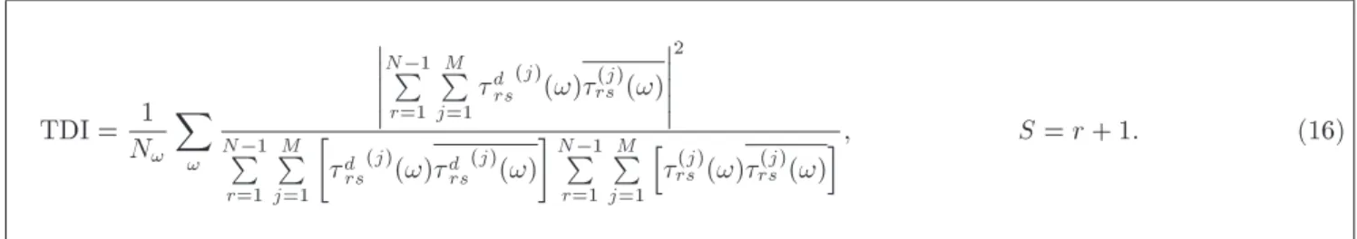
The Transmissibility Damage Indicator is dened by Eq. (16), as shown in Box II, where Nw is the
number of frequencies. TDI varies from 0 to 1, from total damage to no damage, respectively.
2.4. Damage detection and quantication using weighted damage indicator
The Weighted Damage Indicator (WDI) is an improve-ment to the TDI, where the values of the MRVAC along the frequency range are taken into consideration together with the number of times that those results happen. The values of the MRVAC are classied in 10 intervals of 0.1 (MRVAC values from 1 to 0.9, 0.9 to 0.8,..., 0.1 to 0). For each interval i, the contribution of the MRVAC value is given by:
P
ni
j=1MRVACj
i
N ; (17)
where ni is the number of recorded observations, and
the incidence of the number of occurrences in each
MRVAC(!) =
N 1P r=1
M
P
j=1 d
rs(j)(!)rs(j)(!)
2
N 1P r=1
M
P
j=1
d
rs(j)(!)drs(j)(!)
N 1P
r=1 M
P
j=1
h
rs(j)(!)rs(j)(!)
i; S = r + 1: (15)
TDI = N1
!
X
!
N 1P r=1
M
P
j=1 d
rs(j)(!)rs(j)(!)
2
N 1P r=1
M
P
j=1
d
rs(j)(!)drs(j)(!)
N 1P
r=1 M
P
j=1
h
rs(j)(!)rs(j)(!)
i; S = r + 1: (16)
Box II interval is ni=N. Therefore, a possible indicator of
damage in each interval i is: Ai=
P
ni
j=1MRVACji
N
ni
N; (18)
which is 1 when there is no damage and 0 when there is total damage. To give more expression to the small values and less expression to the big ones, Eq. (18) is modied as follows:
Ai=(P ni
j=1MRVACj)i
N
m
nNi; (19) where m > 1. Adding ten intervals, the weighted damage indicator is dened as follows:
WDI =X10
i=1
Ai= Nm+11 10
X
i=1
(ni (Sumi)m); (20)
where: Sumi= (
ni
X
j=1
MRVACj)i: (21)
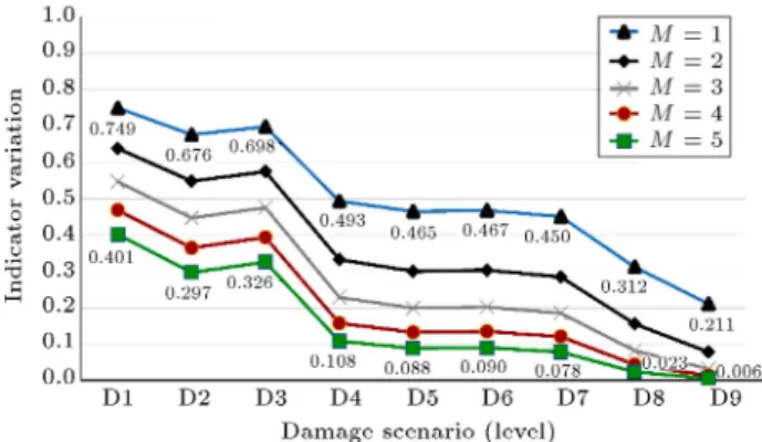
In Section 4, one can verify that an increase in exponent m allows an earlier detection of small damages. Five dierent values for exponent m, 1 to 5, have been tested.
3. Application example
A steel beam with a constant rectangular cross-section was considered. Figure 1 shows the structure used in this study. The dimensions of the beam are 1.002 m in length, 0.035 m in width, and 0.006 m in thickness.
Nine levels of damage, D1 to D9, were considered. To simulate an actual damage condition, a saw cut was made between coordinates 15 and 16 at L1 =
728:5 mm, as shown in Figure 1. The width of the crack was kept constant and equal to 1.5 mm. Cut depth d varied from 0.5 mm to 5 mm. The damaged scenarios are dened as scenarios D1-D9 in Table 1. Three damages are shown in Figure 2.
Firstly, a numerical study based on the Finite-Element Method was carried out. Then, the experi-mental modal testing was completed.
Figure 1. Beam test specimen.
Table 1. The nine damage scenarios. Scenario
Saw cut (width) (mm)
Saw cut (depth) (mm)
D1 1.5 0.5
D2 1.5 1
D3 1.5 1.25
D4 1.5 1.6
D5 1.5 3
D6 1.5 3.5
D7 1.5 4
D8 1.5 4.5
D9 1.5 5
4. Numerical analysis
To verify the eectiveness of the damage detection algo-rithms, introduced in Section 2, from a numerical point of view, the numerical modal analysis based on the nite-element package FEMAP-MSC/NASTRAN was used to simulate the procedure corresponding to the experimental operation. Figure 3 shows the 3D Finite-Element Model used to simulate a beam, considered as the reference structure. The geometry of the beam was assumed as a plate with 0.035 m width, 1.002 m length, and 0.006 m thickness. The meshes consist of 32064 CHEXA elements. The elastic modulus and the density of all parts are E = 1:8905 109 Pa and = 7:860
Figure 2. Examples of the induced damages: (a) D1 (saw cut depth = 0.5 mm), (b) D5 (saw cut depth = 3 mm), and (c) D8 (saw cut depth = 4.5 mm).
Figure 3. Original mesh and location of accelerometers: (a) Original mesh, and (b) accelerometer locations. simulated by FEM analysis using MSC/NASTRAN, applying a unitary impulse load on point No. 3 of the panel; 23 FRFs were computed in the range of 1{800 Hz, with a frequency resolution of 0.25 Hz for 23 selected grids (red color nodes), representing the locations of accelerometers (corresponding to the same point on experimental testing) on the mentioned structure. In this study, to validate and correct the initial FE beam model, a correlation analysis between numerical and experimental beam data is considered for the healthy beam. Generally, correlation analysis is a technique to examine quantitatively and qualitatively the correspondence and dierence between analytically and experimentally obtained modal parameters [20]. Dynamic responses, namely natural frequencies and mode shapes, were used as the indices for the objective function (that must be minimized) of the correlation analysis. In this case, rst, for the mode shape vectors, the Modal Assurance Criterion (MAC) was adopted to make a comparison between numerical and experimental mode shapes. The initial ErrF revalues of
the natural frequencies of the rst seven exural modes are reported in Table 2. Besides the ErrF re values,
also displayed are the absolute dierences between
numerically and experimentally obtained frequencies prior to the optimization procedure [20].
Finally, Table 3 shows a comparison between the initial (before updating) and nal (after updating) design variables. According to the result of the opti-mization in Table 4, it was inferred that the numerical model simulates the experimental model quite well, and they are matched very well. Therefore, the optimized model of the beam can be used in the next two sections as a representation of the experimental beam structures for application of the proposed damage identications techniques.
The nine damaged scenarios (D1-D9 according to Table 1) were simulated by removing the necessary elements of the beam. For each scenario, the FRF input matrix was generated. In order to simulate an actual measurement, the responses were polluted with a level of 3% random noise. The responses at all frequencies, for each damage scenario, were used to calculate, GDI3P C, DIT2, TDI, and WDI
indicators. Figure 4 shows the results obtained with the application of GDI3P Cdamage indicator for all damage
cases, without noise and with 3% added random noise. Figure 5 shows the results obtained with the application of DIT2 damage indicator for all damage
cases, without noise and with 3% added random noise. Figure 6 shows the results obtained with the Table 3. Optimization analysis results of beam. Design
variable
Initial value
Final value
Dierence (%) E beam 2:10 1011 1:89 1011 10.00
Table 2. Comparison of the natural frequencies between numerical and experimental beam data before updating. Mode
(#)
Experimental beam
(Hz)
Numerical beam
(Hz)
Absolute dierence
(Hz)
ErrF re
(%)
1 30.06 31.75 1.68 5.60
2 81.52 87.51 5.99 7.34
3 160.53 171.55 11.02 6.86
4 265.72 283.56 17.83 6.71
5 395.10 423.56 28.46 7.20
6 551.63 591.54 39.91 7.23
Table 4. Comparison of the natural frequencies between numerical and experimental beam data after updating. Mode
(#)
Experimental beam (Hz)
Numerical beam (Hz)
Absolute dierence (Hz)
ErrF re
(%)
1 30.06 29.80 0.26 0.87
2 81.52 82.14 0.61 0.75
3 160.53 161.00 0.47 0.30
4 265.72 266.11 0.38 0.14
5 395.10 397.45 2.35 0.59
6 551.63 554.98 3.35 0.61
7 732.53 738.66 6.41 0.88
Figure 4. Result obtained with the 3PC GDI indicator for all damage levels using simulation data: (a) Without noise, and (b) 3% added noise.
Figure 5. Result obtained with the DIT2indicator for all damage levels using simulation data: (a) Without noise, and
(b) 3% noise.
Figure 6. Result obtained with the TDI indicator for all damage levels using simulation data: (a) Without noise, and (b) 3% noise.
Figure 7. Result obtained with the WDI indicator for all damage levels using simulation data: (a) Without noise, and (b) 3% noise.
application of TDI damage indicator for all damage cases, without noise and with 3% added random noise. Figure 7 shows the results obtained with the application of WDI damage indicator for all damage cases, without noise and with 3% added random noise. The results observed in Figures 4-7 show that all the proposed methods, with the exception of GDI3P C,
can detect all damages very well. As seen in Figures 5 and 6, a small level of the damages is not so easily detectable with TDI and (DIT2) indicators, while the
other two indicators improve the early detection of damage, as they seem able to detect low levels of damage, which is of signicance in critical situations. In the case of W DI indicator, this improvement is more evident when higher values of m exponent are used. The choice of the value of this exponent is directly related to the eect that the damage may have on the structure under study, being especially important for critical structures where the damages should be detected as early as possible. In addition, it is possible to see that all the damage indicators remain stable even in the presence of noise, thanks to the ltering capability of these methods.
5. Experimental testing
The experimental testing was carried out on free-free boundary conditions by suspending the beam using elastic bungees. Twenty-three equally spaced points for translation response measurements were considered, and the test item was excited pseudo-randomly by a Bruel & Kjaer 4809 shaker, powered by a Bruel & Kjaer 2706 power amplier at several locations. In each test session, four excitation forces were applied at points 3, 7, 12, and 19, one at a time. The force was transmitted through a stinger and measured by a Bruel & Kjaer 8200 force transducer. The responses were measured by 23 CCLD accelerometers. The signals were fed into the Multi-Channel Data Acquisition Unit Bruel & Kjaer 2816 (PULSE) and analyzed directly with the Labshop 6.1 Pulse software from the attached laptop
Figure 8. Result obtained with the 3PC GDI indicator for all damage levels using experimental data.
(Dell series 400). The frequency analysis of the beam was 0-800 Hz containing a frequency resolution equal to 0.25 (3200 lines), Hanning windows for force and responses, and 15 averages to obtain the accelerations. Figure 1 shows the location of the shaker as well as the 23 xed accelerometers. Again, nine various damage scenarios have been analyzed, and the FRF input matrix was measured for each scenario. The responses at all frequencies, for each damage scenario, were used to calculate GDI3PC, DIT2, TDI, and WDI
indicators. Figure 8 shows the results obtained with the application of GDI3PCdamage indicator for all damage
levels using experimental testing data.
Figure 9 shows the results obtained with the application of (DIT2) damage indicator for all damage
levels using experimental testing data.
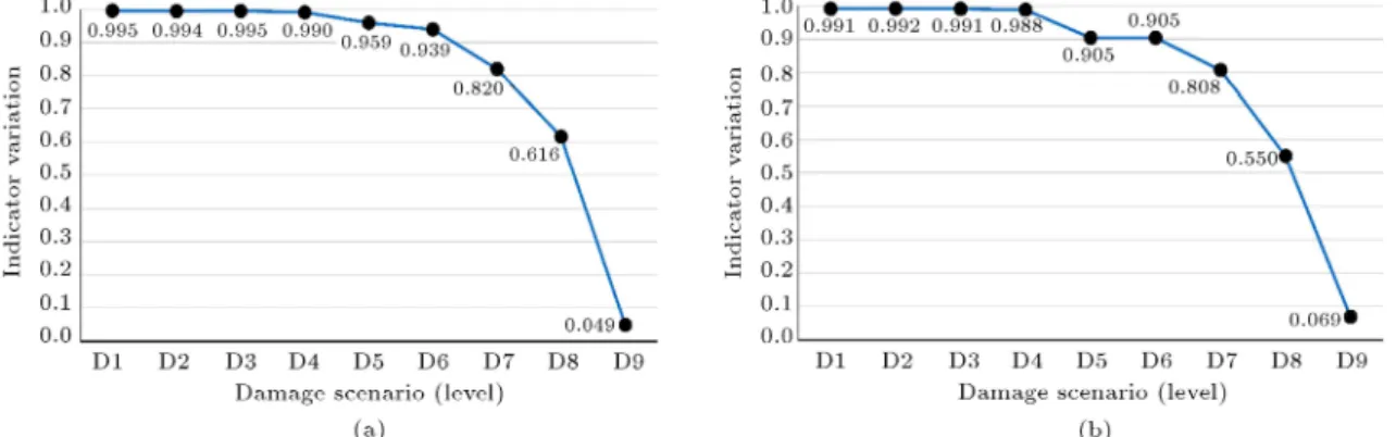
Figure 10 shows the results obtained with the application of TDI damage indicator for all damage levels using experimental testing data.
Figure 11 shows the results obtained with the application of WDI damage indicator for all damage levels using experimental testing data.
The results observed in Figures 8-11 show that all the proposed methods can detect and dierentiate all damages reasonably well. As one can see in Figure 8, GDI3PC is the method that is more inconsistent. In
Figure 9. Result obtained with the DIT2 indicator for all
damage levels using experimental data.
Figure 10. Result obtained with the TDI indicator for all damage levels using experimental data.
Figure 11. Result obtained with the WDI indicator for all damage levels using experimental data.
general, the experimental results are coherent with the numerical ones.
6. Conclusions
The present study focuses on the detection and relative quantication of damage using the frequency response functions obtained from experimental modal testing. The tested item is a simple beam under freely sup-ported conditions. A numerical Finite-Element (FE) analysis was performed to complement the study and demonstrate the validity of the damage identication
algorithms. Two new damage indicators, GDI3PC and
DIT2, were developed, and the results compared with
TDI, and WDI are presented in [24]. The following major conclusions can be highlighted:
- All the mentioned damage indicators (GDI3PC,
DIT2) based on PCA and TDI, WDI based on the
RVAC correlation factor) are readily available from the measurements. This is very useful because it means that they need neither any modal identi-cation nor any analytic or numerical model of the structure; all of them use directly the frequency response functions without any further treatment or analysis;
- The WDI indicator takes into consideration the correlation values along the frequency range, as well as the number of times they occur, leading to results that are more sensitive as compared to the others for the detection and relative quantication of damage, especially in an early detection stage;
- All the damage indicators are robust enough with respect to noise, thanks to the ltering capability of these methods;
- From all the tested indicators, GDI3PC indicator
is the one that provides the weakest results when applied to the experimental case;
- Developed methods are robust and ecient and are able to predict structural conditions by analyzing dynamic data changes. The introduced methods require only minimal measurement information to detect damages in structures precisely;
- Several damage detection algorithms are employed to extract the data from the beam specimens testing, and all of them require both healthy and damaged data information to detect the damage.
References
1. Doebling, S.W., Farrar, C.R., Prime, M.B., and She-vitz, D.W. \Damage identication and health monitor-ing of structural and mechanical systems from changes in their vibration characteristics: a literature review", Los Alamos National Laboratory Report LA-13070-MS, (1996).
2. Doebling, S.W., Farrar, C.R. and Prime, M.B. \A sum-mary review of vibration-based damage identication methods". The Shock and Vibration Digest, 30(2), pp. 91-105 (1998).
3. Alvandi, A. and Cremona, C. \Assessment of vibration-based damage identication techniques", Journal of Sound and Vibration, 292, pp. 179-202 (2006).
4. Bandara, R.P., Chan, T.H.T., and Thambiratnam, D.P. \Frequency response function based damage iden-tication using principal component analysis and pat-tern recognition technique", Engineering Structures, 66, pp. 116-128 (2014).
5. Farrar, C.R., Doebling, S.W., and Nix, D.
\Vibration-based structural damage identication. The royal society-philosophical transactions", Mathe-matical, Physical and Engineering Sciences, 359, pp. 131-149 (2001).
6. Montalvao, D., Maia, N.M.M., and Ribeiro, A.M.R. \A summary review of vibration-based damage identi-cation methods". Shock and Vibration Digest, 38(4), pp. 295-324 (2006).
7. Santos, J.V.A., Maia, N.M.M., Soares, C.M.M. and Soares, C.A.M. \Structural damage identica-tion: a Survey", Chapter 1 of Trends in Com-putational Structures Technology, B.H.V. Topping and M. Papadrakakis, Editors, Saxe-Coburg Publica-tions, Stirlingshire, Scotland, 19(1), pp. 1-24, (2008). DOI:10.4203/csets
8. Pandey, A.K., Biswas, M., Samman, M.M. \Damage detection from changes in curvature mode shape", Journal of Sound and Vibration, 142, pp. 321-332 (1991).
9. Sampaio, R.P.C., Maia, N.M.M., and Silva, J.M.M. \Damage detection using the frequency-response-function curvature method", Journal of Sound and Vibration, 226(5), pp. 1029-1042 (1999).
10. Friswell, M.I. \Damage identication using inverse methods", Philosophical Transactions of the Royal Society, A 365, pp. 393-410 (2007).
11. Liu, X., Lieven, N.A.J., and Escamilla-Ambrosio, P.J. \Frequency response function shape-based methods for structural damage localization", Mechanical Systems and Signal Processing, 23, pp. 1243-1259 (2009).
12. Ray, L.R., Tian, L. \Damage detection in smart struc-tures through sensitivity enhancing feedback control," Journal of Sound and Vibration, 227(5), pp. 987-1002 (1999).
13. Zhou, Y-L, Perera, R., and Sevillano, E. \Damage identication from power spectrum density transmissi-bility", Proceedings of the 6th European Workshop on Structural Health Monitoring, Dresden, Germany (July 2012)
14. Zhou, Y-L. and Perera, R. \Transmissibility based damage assessment by intelligent algorithm", Proceed-ings of the 9th European Conference on Structural Dynamics, (EURODYN), Oporto, Portugal (2014).
15. Zhao, X.Y., Lang, Z.-Q., Park, G., Farrar, C.R., Todd, M.D., Mao, Z., and Worden, K. \A new transmissi-bility analysis method for detection and location of Prediction of fatigue life in cold expanded fastener
holes subjected to bolt tightening in Al alloy 7075-T6 plat", IEEE/ASME Transactions on Mechatronics, 20(4), pp. 1933-1947 (2015).
16. Jollie, I.T., Principal Component Analysis, Springer-Verlag, New York (2002).
17. Bishop, C.M., Neural Networks for Pattern Recogni-tion, Oxford University Press, Oxford (1995)
18. Jackson, J.E., A User's Guide to Principal Compo-nents, John Wiley, New York (1991).
19. Wise, B.M., Gallagher, N.B., Butler, S.W., White, D.D., and Barna, G.G. \Development and benchmark-ing of multivariate statistical process control tools for a semiconductor etch process: Impact of measurement selection and data treatment of sensitivity", IFAC Safe Process, pp. 35-42 (1997).
20. Rezvani, K. \Vibration-based damage identication techniques", PHD Thesis. Italy: Politecnico di Milano (2015).
21. Rezvani, K. and Ricci, S. \Using principal component analysis for damage detection of aerospace structures", Italian Association of Aeronautics and Astronautics XXII Conference, Napoli, pp. 9-12 (Sep. 2013).
22. Qin, S.J. \Statistical process monitoring: basics and beyond", J. Chemometrics, 17, pp. 480-502 (2003).
23. Ribeiro, A.M.R., Maia, N.M.M., and Silva, J.M.M. \On the generalisation of the transmissibility concept", Mechanical Systems and Signal Processing, 14(1), pp. 29-35 (2000)
24. Fontul, M., Ribeiro, A.M.R., Silva, J.M.M., and Maia, N.M.M. \Transmissibility matrix in harmonic and random processes", Shock and Vibration, 11, pp. 563-571 (2004).
25. Maia, N.M.M., Almeida, R.A.B., Urgueira, A.P.V., Sampaio, R.P.C. \Damage detection and quantica-tion using transmissibility", Mechanical Systems and Signal Processing, 25, pp. 2475-2483 (2011).
26. Heylen, W., Lammens, S., and Sas, P. Modal Analysis Theory and Testing, Katholieke Universiteite Leu-ven, Faculty of Engineering, Department of Mechan-ical Engineering, Division of Production Engineering, Machine Design and Automation, Leuven, Belgium (1998).
Biographies
Kamal Rezvani was a PhD student graduated from Politecnico di Milano, the Department of Science and Technology of Aerospace, Italy. He is working on Vibration-Based Damage Identication Techniques. He obtained his rst undergraduate degree in Me-chanical Engineering from Islamic Azad University in 2007. During his undergraduate studies, he learned the fundamental mechanical principles. After that, he continued his education at the same university to re-ceive his MS degree in the eld of Engineering-Applied Design with specialty in modeling the metal forming.
Dr. Rezvani not only did a lot of research on modelling and simulation of dynamic processing with dierent methods (like FEM and Experimental), but also did some research on damage and fracture phenomenon. It should be noted that he was a successful student during his Bachelor and Master programs, known to be a distinguished student. Now, Dr. Rezvani is a Postdoctoral Fellow in Aerospace Engineering in the Faculty of New Sciences & Technologies, University of Tehran.
Nuno Manuel Mendes Maia obtained his BS and MS degrees (1978 and 1985, respectively) in Mechanical Engineering from Instituto Superior Tecnico (IST), Technical University of Lisbon (TU Lisbon). He re-ceived his PhD degree in Mechanical Vibrations (1989) from Imperial College, University of London, UK. He had his habilitation in Mechanical Engineering (2001) from Instituto Superior Tecnico, Technical University of Lisbon, TU Lisbon. Dr. Maia has authored around 80 international conferences on the subject of modal analysis and structural dynamics since 1998. He is an Associate Editor of the Shock and Vibration Journal,
a member of the Society for Experimental Mechanics (SEM), a member of the International Institute of Acoustics and Vibration (IIAV), and of the Portuguese Society of Acoustics (SPA), where he is responsible for the area of vibrations. Currently, he supervises 5 PhD students; he has participated and coordinated various national and international research projects in the area of modal analysis and structural vibrations. As the chairman of the International Conference on Structural Engineering Dynamics (ICEDyn), he is responsible for organizing the conference. His current research inter-ests are modal analysis and modal testing, updating of nite-element models, coupling and structural mod-ication, damage detection in structures, modeling of damping transmissibility in multiple degree-of-freedom systems, and force identication.
Mohammad Hossein Sabour obtained his BS de-gree (1990) in Mechanical Engineering from University of Tehran. Also, he obtained his MS degree (1993) in the same eld from Tarbiat Modares University, and his PhD degree in Aerospace Engineering (2005) from Concordia University, Canada.