Numerical Simulations of the Ram Pressure-Driven Rayleigh-Taylor
Instability
Maggie Hilderbran
April 2, 2019
Abstract
Star formation in the Galactic disk is fueled by continuous accretion of gas from the Galactic halo. This infalling gas is usually identified in the form of high-velocity clouds (HVCs), so named because their velocities do not match a standard Galactic rotation pattern. As they pass through the halo, HVCs are disrupted by a series of fluid instabilities. The Rayleigh-Taylor instability (RTI), driven by ram pressure, occurs at the interface between the cold, dense cloud and the hot, diffuse halo. I perform a systematic investigation of the RTI under conditions relevant to HVCs in the halo, exploring how the instability contributes to the breakup of these clouds. I use the grid-based fluid dynamics code Athena (Stone et al. 2008) to solve the equations of ideal magnetohydrodynamics, simulating the instability at the halo-cloud interface. Step-by-step addition of radiative processes and magnetic fields provides an understanding of their effects on the evolution of the RTI. Cooling causes rapid fragmentation of the interface and dampens the instability, in line with Vietri et al. (1997). The addition of a uniform magnetic field suppresses the instability in two dimensions but not in three dimensions, consistent with Stone & Gardiner (2007). In contrast, tangled magnetic fields, which may be a more realistic model, produce results more like the hydrodynamical case. Because the plane-parallel geometry I assume does not take into account mass flow around (and away from) the interface, the instability growth found in my models is likely an upper limit compared to more realistic situations.
1
Introduction
Star formation in the Galactic disk is fueled by continuous accretion of gas from the Galactic halo. This infalling gas is usually identified in the form of high-velocity clouds (HVCs), so named because their velocities are inconsistent with a standard Galactic rotation pattern. HVCs are typically defined as having speeds differing from the local standard of rest by at least 90 km s−1(Wakker & van Woerden 1997).
Yet despite their significance for Galactic evolution, the origin of HVCs remains uncertain. Wakker & van Woerden (1997) argued that given the observed diversity of these clouds, multiple origin hypotheses should be considered: one for the Magellanic Stream, another for clouds in the “Outer Arm Extension,” and one or more for other HVCs. The fountain model and accretion from dwarf galaxies and/or the intergalactic medium are among the central theories. In the fountain model, Shapiro & Field (1976) proposed that hot (T ∼ 106K) gas in the interstellar medium (ISM) rises into the Galactic halo, where it cools through
radiation and condenses into clouds that fall back to the disk at high velocities (see also Bregman 1980). Alternatively, HVCs may be the result of accretion of intergalactic gas, either remaining from the formation of our galaxy (Oort 1966, 1970) or pulled from satellite galaxies (e.g., the Magellanic Clouds) via tidal forces or ram pressure stripping (Wakker & van Woerden 1997). These hypotheses are not mutually exclusive: in a more recent numerical investigation of the HVC complex C, Fraternali et al. (2015) brought together the fountain and accretion models, demonstrating that both ejection of hot gas from the galactic disk and accretion of external gas could explain the formation of the cloud.
scenarios; however, mixing with and accretion of ambient halo material present challenges for interpreting the measurements.
Related to the question of cloud origin is that of cloud survival. During their passage through the Galactic halo, HVCs interact with the ambient gas through a series of fluid instabilities. Simulation results have consistently suggested that under conditions typical for HVCs, the clouds should be disrupted quickly enough to raise the question of why we actually observe so many of them. For example, Quilis & Moore (2001) and Heitsch & Putman (2009) both show that typical HVCs would not survive passage through the halo to make it to the Galactic disk. While Forbes & Lin (2018) implicitly suggest that the usual numerical experiments are over-idealized by omitting a warm envelope around the cold cloud, here, I take a closer look at one of the fluid instabilities supposed to drive the disruption of HVCs.
The Rayleigh-Taylor instability (RTI), driven by ram pressure, occurs at the interface between the cold, dense cloud and the hot, diffuse Galactic halo. I perform a systematic investigation of this instability, beginning with minimal assumptions about the physical processes, then adding step-by-step the physics relevant to the regime in which HVCs are found. I use the grid-based fluid dynamics code Athena (Stone et al. 2008) to solve the equations of ideal magnetohydrodydnamics (MHD), simulating the instability and its growth at the halo-cloud interface.
1.1
The Rayleigh-Taylor Instability
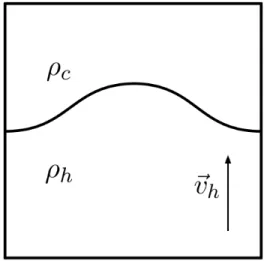
The RTI occurs when a denser fluid is accelerated against a less dense fluid (Figure 1). Perturbation of the interface between the two fluids results in growth of the instability and mixing of the fluids.
The physical processes underlying the instability are best understood through the gravity-driven RTI. Figure 1a shows the initial conditions for the gravity-driven RTI, where ρ2 is the density of the heavier
fluid andρ1 is the density of the lighter fluid, and F~G is the gravitational force given by the gravitational
acceleration~g, which acts downwards. The interface between the two fluids is unstable, since it is energetically less favorable to have the heavier fluid at a higher gravitational potential energy than the lighter fluid. Thus, when the interface is perturbed, the instability will grow and the fluids will begin to mix, eventually switching places as the denser fluid falls down below the less dense fluid.
Alternatively, ram pressure, rather than gravity, can drive the RTI. Figure 1b shows the ram pressure-driven instability in the context of high-velocity clouds, where a dense cloud of gas moves through the diffuse Galactic halo. The densitiesρc andρhdenote the cloud and halo gas, respectively, and~vhis the velocity of
the halo gas relative to the interface. The ram pressure from the inflow of halo gas drives the instability.
(a) The classical, gravity-driven instability. (b) The ram pressure-driven instability.
Figure 1: Two models for the RTI.
below the interface andρ2above, perturbations to the densityρ, pressureP, and velocityv at the interface
can result in instability. For the RTI,P andρdepend only uponz.
The hydrodynamical evolution of a fluid in an Eulerian reference frame can be written in the form of conservation laws. Mass conservation is described by
∂tρ+∇(ρv) = 0, (1)
where ρis the density andv is the vector-valued velocity of the fluid, and momentum conservation can be expressed as
∂t(ρv) +∇(ρvv) =−∇P−ρgz (2)
where P is the pressure of the fluid. Here, the fluid is assumed to be inviscid. Linear perturbations are introduced into the quantitiesρ,P, and v:
ρ=ρ0+δρ (3)
P=P0+δP (4)
v=δv, (5)
where the perturbation of v is simply δv because v0 is defined to be zero (the interface is at rest). For
discontinuities in density at some positionszs(fors= 1, 2, 3, etc.), the interface position is then
zs+δzs(x, y, t). (6)
Applying Equations 1 and 2 to the perturbations, the condition for mass conservation (along the z -direction) becomes
∂tδρ+vz∂zρ0= 0. (7)
Momentum conservation yields
ρ0∂tvx=−∂xδP (8)
ρ0∂tvy=−∂yδP (9)
ρ0∂tvz=−∂zδP−gδρ+
X
s
Ts
∂2
∂x2 +
∂2
∂y2
δzs
δ(z−zs), (10)
where Ts is the surface tension. The last term in Equation 10 comes from the discontinuity in the normal
stresses as required for equilibrium,
Ts
∂2
∂x2 +
∂2
∂y2
δzs. (11)
The fluid is taken to be incompressible (such that∇ ·v= 0):
∂xvx+∂yvy+∂zvz= 0. (12)
We look for solutions for δP,δρ, andv dependent uponx, y, and tin the form exp (ikxx+ikyy+nt),
where kx and ky are the wavenumbers for modes in the x- and y-directions, respectively, and n is the
frequency or growth rate. IfP,ρ, andvare dependent uponx,y, andtin this manner, then Equations 7- 10 and 12 become
nδρ=−vz∂zρ0, (13)
nρ0vx=−ikxδP (14)
nρ0vy =−ikyδP (15)
nρ0vz=−∂zδP−gδρ−k2
X
s
(Tsδzs)δ(z−zs) (16)
ikxvx+ikyvy=−∂zvz (17)
wherek=qk2
Equations 14, 15, and 17 can be solved together to obtain
k2δP =−nρ0
d
dzvz
, (18)
while combination of Equations 13 and 16 yields
d
dzδP =−nρ0vz+
g n
d
dzρ0
vz−
k2
n
X
s
(Tsvz,s)δ(z−zs), (19)
whereδzs has been replaced byvz,s/n.
By eliminatingδP from Equations 18 and 19, the following governing equation is obtained:
d dz
ρ0
d
dzvz
=k2
" − g
n2
d
dzρ0
+k
2
n2
X
s
Tsδ(z−zs)
!
vz+ρ0vz
#
. (20)
Forz 6=zs, the surface tension terms in these equations disappear. However, at the interface between the
two fluids, integration of Equation 18 over a infinitesimal length aroundzs gives
k2∆s(δP) = ∆s
−nρ0
d
dzvz
, (21)
where ∆s(f) = f(zs+ 0)−f(zs−0) represents the jump in a quantity f across the interface at zs. For
Equation 19, integration across the surface yields
∆s(δP) =
g
nvz,s∆s(ρ0)−
k2
nTsvz,s. (22)
Combining Equations 21 and 22 results in the following jump condition for the interface between the fluids:
∆s
ρ0
d
dzvz
=−k
2
n2
g∆s(ρ0)−k2Ts
vz,s. (23)
Equation 20 is true for all positions except z=zs, where Equation 23 is the governing equation. Setting
vz = 0 on the boundaries, the conditions from Equations 20 and 23 can be applied to obtain a dispersion
relation forn.
For two fluids of uniform densities separated by a horizontal boundary at z= 0, nis given by
n2=gk
ρ
2−ρ1
ρ2+ρ1
− k
2T
g(ρ2+ρ1)
, (24)
where T is the surface tension (Chandrasekhar 1961). Instability occurs when n is real (that is, when
ρ2> ρ1). For configurations withρ1> ρ2, nis imaginary and stability is achieved.
If there is no surface tension (T = 0), the system is unconditionally unstable, and the growth of the perturbation amplitude due to the growth ratenis
exp (nt) = exptpgkA, (25)
with the Atwood numberA
ρ2−ρ1
ρ2+ρ1
. (26)
The above reasoning applies to not only the gravity-driven RTI but also the ram pressure-driven insta-bility, in which the acceleration of the heavier fluid against the lighter one is caused by ram pressure rather than by gravity. As dense gas moves in a diffuse medium, the relative velocityvof the diffuse gas results in ram pressure
In the case of a dense cloud (ρc) moving through diffuse gas (ρh), as shown in Figure 1b, this ram pressure
corresponds to a drag forceFD, which causes an accelerationaD:
aD=
FD
Mcloud
=1 2cw
Pram
Σcloud
, (28)
whereMcloudis the cloud mass,cwis the drag coefficient, and Σcloudis the mean column density of the cloud
(Roediger & Hensler 2008). In the ram pressure-driven instability, this acceleration from the drag force acts like the gravitational acceleration in the gravity-driven RTI.
In my idealized simulation setup, the expression for the acceleration due to ram pressure simplifies further due to the assumption of a plane-parallel geometry—instead of exploring the whole cloud, I focus on the leading surface interacting with the ambient gas. For this specific case,
aD=
ρv2
Σ , (29)
where Σ is the surface density of the denser gas andρv2 is the ram pressure exerted on the dense gas by the
diffuse gas.
1.2
The Effects of Heating and Cooling
To accurately model the evolution of the RTI at the edge of a high-velocity cloud in the Galactic halo, I include the effects of heating and radiative cooling processes that occur in interstellar gas.
For the RTI, the reasoning behind the effects of radiative losses parallels that given by Vietri et al. (1997) for the Kelvin-Helmholtz instability. When the cooling timescale in a region is shorter than the dynamical (sound crossing) time, the instability cannot propagate and therefore should remain relatively contained near the interface. Their numerical simulations indeed show confinement of the instability, as well as that turbulence at the cloud’s edges generally does not easily reach the rest of the cloud (Vietri et al. 1997).
I anticipate similar conditions for the RTI: radiative losses due to cooling should create a damping effect, reducing the instability’s growth and resulting in a more compressed, fragmented interface between the halo and cloud gas. The cooling gas may act as a mass sink as well, causing accretion.
Interstellar gas is heated and cooled through a wide array of physical processes (e.g., Dalgarno & McCray 1972), effectively leading to two or three coexisting regimes of density-temperature pairs, or “phases,” that are in approximate pressure equilibrium (McKee & Ostriker 1977). Calculations by Wolfire et al. (1995) of the ISM thermal equilibrium temperature show this two-phase structure: the warm neutral medium (WNM) and the cold neutral medium (CNM) exist in pressure equilibrium, both with thermal pressures P/kB '
103-104K cm−3 (Wolfire et al. 1995).
Koyama & Inutsuka (2000) provided more accurate calculations of the equilibrium temperature by ad-ditionally accounting for the effects of the formation and cooling of H2 and CO. The following heating
processes are included in their calculations: photoelectric heating from small grains and polycyclic aromatic hydrocarbons, ionization heating by cosmic rays and x-rays, and heating from the formation and dissociation of H2. For cooling, they account for atomic lines (Lyα, C II, O I, Fe II, and Si II), H2and CO ro-vibrational
lines, and collisions of atoms and molecules with grains.
Koyama & Inutsuka (2002) provide a compact fit expression to the energy change rate
˙
E=nΓ−n2Λ, (30)
wherenis the gas number density. I use their heating and cooling functions in my model. The cooling rate Λ, with typographical corrections given by V´azquez-Semadeni et al. (2007), is
Λ(T) Γ = 10
7exp
−1.184×10⁵
T+ 1000
+ 1.4×10⁻² √
Texp
−92
T
cm3, (31)
where T is given in Kelvin. The two cooling processes dominating the radiative losses are Lyαand [C II] emission.
The heating rate Γ is
The model of heating and cooling given by Wolfire et al. (1995) reflects a stable, two-phase interstellar medium. I set the initial density conditions of my model (Sec. 2.2.1) to be consistent with these phases, such that the halo and cloud gas are in thermal equilibrium and the pressure is constant across the simulation domain.
1.3
The Effects of Magnetic Fields
Chandrasekhar (1961) also analyzed the RTI in the case of magnetic fields both perpendicular to and parallel to the interface between the fluids.
A fieldB~ parallel to the interface produces an effective surface tension
Teff=
B2
2πkcos
2θ, (33)
where θis the angle between the wavevector~k= (kx, ky) and the magnetic fieldB~ (Chandrasekhar 1961).
Modes perpendicular to B~ have an effective surface tensionTeff = 0. The magnetic field, therefore, has no
impact on the growth of these modes.
For modes parallel to B~ (having a non-zeroTeff), the condition for realngiven by Equation 24 is
ρ2−ρ1
ρ2+ρ1
> k
2T eff
g(ρ2+ρ1)
, (34)
yielding a critical wavenumber
k2c =
2πgk(ρ2−ρ1)
B2 . (35)
Above this critical wavenumber, the instability will be suppressed for modes parallel toB~. This wavenumber corresponds to a critical wavelength
λc=
2π kc
= B
2
g(ρ2−ρ1)
. (36)
Forλ < λc,nis imaginary, yielding oscillatory but stable solutions. Forλ > λc, the instability will grow.
The critical field strength for an interface of lengthL is therefore
Bc=
p
Lg(ρ2−ρ1). (37)
At field strengthsB > Bc, the instability will be suppressed; B must be be smaller than Bc for growth to
occur.
2
Method
To study the RTI evolution in the context of high-velocity clouds, I simulate a ram pressure-driven instability. I focus on the interface at which the instability occurs, rather than modeling the HVC in its entirety. The HVC is represented by the dense gas, and the galactic halo is represented by an inflow of diffuse gas, creating ram pressure that accelerates the dense cloud gas. I apply a perturbation to the halo-cloud interface and study the evolution of the resulting RTI.
2.1
Athena
2.1.1 Equations Solved
As given by Stone et al. (2008), Athena solves the following equations of ideal MHD:
∂ρ
∂t +∇ ·(ρv) = 0, (38)
∂ρv
∂t +∇ ·(ρvv−BB+ P
∗) = 0, (39)
∂E
∂t +∇ ·[(E+P
∗)v−B(B·v)] = 0, (40)
∂B
∂t − ∇ ×(v×B) = 0, (41)
where the diagonal tensorP∗ has componentsP∗=P+B2/2 and the total energy densityE is
E= P
γ−1 +
1 2ρv
2+B
2
2 , (42)
with B2 = B·B (Stone et al. 2008). The magnetic permeability µ is equal to 1 in the units of these
equations. To obtain Equation 42, Athena uses an equation of state for an ideal gas, given by
P = (γ−1)e, (43)
where γ is the specific heat ratio and e is the internal energy density (Stone et al. 2008). I use γ = 5/3, corresponding to a monatomic gas.
2.1.2 Units
Athena performs calculations in its own system of computational units, which defines the following constants:
• G= 1, [G] = cm3g−1 s−2
• kb= 1, [kb] = erg K−1
Quantities in Athena’s computational unit system can be converted to physical units:
qphys=q0·qcu, (44)
whereqphysis the quantity measured in physical units,q0is the conversion factor, andqcuis the quantity in
computational units.
The conversion factors used for conversion from computational to CGS units are given in Table 1. When applicable, the conversion factors are also provided in more relevant units.
2.1.3 Comoving Frame
To keep the interface between the dense and diffuse gas within the simulation domain, I use a comoving frame of reference that shifts to follow the interface, which is pushed in the +y (three dimensions: +z) direction by ram pressure from the inflow of diffuse halo gas.
I track the interface via a scalar fieldS0. The interface velocityvint is then the center-of-mass upwards
velocity:
vint =
P
i,jvy[i, j]·S0[i, j]
P
i,jS0[i, j]
. (45)
From the interface velocity vint I determine a velocity correction ∆v, which increases with the distance
between the interface and its intended central position:
∆v=vint
|yCOM|
0.3ly
quantity conversion factor CGS value equivalent value
density n0 1 cm−3
temperature T0 1 K
time t0 3×10¹⁵s 95 Myr
length/position l0 2.724×1019 cm 8.83 pc
velocity v0 9094 cm s−1 0.091 km s−1
pressure P0 1.381×10⁻¹⁶g cm−1 s−2 [Ba] 1 K cm−3(P0/kB)
energy E0 2.79×1042g cm2 s−2 [erg] 2.79×1035J
magnetic field B0 1.17×10⁻⁸ G 0.0117µG
Table 1: Factors for conversion from computational to physical units.
whereyCOM is the center-of-massy-position
yCOM=
P
i,jy[i, j]·S0[i, j]
P
i,jS0[i, j]
. (47)
In three dimensions, ∆v is determined fromvzandzCOM.
The velocity correction ∆v is then subtracted from the whole simulation grid, while simultaneously updating the vertical grid position. Thus, the grid moves with the interface, keeping the interface centered. Corrections are made accordingly to other variables (position, energy, etc.) to account for the velocity change. The upper and lower boundaries are updated with the velocity correction ∆v for the comoving frame as well.
2.2
Simulation Parameters
The simulation domain is of sizeL×2L(three dimensions: L×L×2L), withL= 1.0 = 8.8 pc.
2.2.1 Initial Conditions
In two dimensions, the interface between the dense gas (representing the cloud) and the diffuse gas (representing the halo) is parallel to the x-axis. In the case of a standard sinusoidal perturbation at the halo-cloud interface, the perturbation shape is given by
y(x) = cos 2πx
lx
, (48)
where lx is the length of the simulation domain along the x-axis. To model a random interface, the
per-turbation of the interface is determined by a sum of sinusoidal functions with random phase shifts, such that
y(x) =
kmax X
k=1
k−acos
2π
lx
(kx+φ)
, (49)
wherekmax= 5,a= 1.5, andφis a random number chosen from the uniform distribution U(0,1).
The three-dimensional random interface is given by
z(x, y) = X
kx,ky
r−acos
2π
lx
(kxx+φx)
cos
2π
ly
(kyy+φy)
, (50)
where r =qk2
x+k2y, a = 1.5, and φx,y are k2max random numbers chosen from the uniform distribution
The amplitude of the perturbation is then scaled such that the maximum initial amplitude ya(x) above
y= 0 isA0= 0.1 (= 0.88 pc). To keep the interface shape constant across test runs, I always use the same
seed for random number generation.
The initial density profile is set to ρ=ρc above the interface (for the cloud gas) and ρ=ρh below the
interface (the halo gas). In two dimensions, the density is given by:
ρ(x, y) =ρh+
1
2(ρc−ρh)
1 + tanh y−y
a(x)
ly/Ny
, (51)
whereya(x) is the initial amplitude of the perturbation given by Equation 48 or Equation 49,lyis the length
of the domain along they-axis, andNy is the number of grid cells along they-axis.
The halo and cloud gas are also in ram pressure equilibrium. The initial conditions for velocity establish this equilibrium and set up the inflow of diffuse halo gas, which creates the ram pressure that drives the instability. The velocity in thex-direction is initially set to be zero (three dimensions: x- andy-directions). The vertical velocity vy around the interface is given by the velocity eigenfunction corresponding to the
interface perturbations (Eq. 48 and 49):
vy(x, y) =vh+
1
2(vc−vh)
1 + tanh
y−ya(x)
4ly/N y
+A0exp (−k|x|) exp (−k|y| −ya(x)), (52)
where vh is the velocity of the halo gas, vc is the velocity of the cloud gas, and k is the wavenumber for
sinusoidal waves with spanning the simulation domain in thex-direction:
k= 2π
lx
. (53)
The last term in Equation 52 represents perturbation of the velocity, which drives the instability. In three dimensions, the density profile is similar:
ρ(x, y, z) =ρh+
1
2(ρc−ρh)
1 + tanh z−z
a(x, y)
lz/Nz
, (54)
where the the initial amplitudeza(x, y) comes from Equation 50,lz is the length of the simulation domain
along thez-axis, andNz is the number of grid cells in thez-direction. The vertical velocityvzis the velocity
eigenfunction corresponding to the three-dimensional interface perturbation (Eq. 50):
vz(x, y, z) =vh+
1
2(vc−vh)
1 + tanh z−z
a(x, y)
4lz/N z
+A0exp (−k|x|) exp (−k|y|) exp (−k|z| −za(x, y)), (55)
To prevent an initial “kick” to the interface, the halo and cloud gas are set up in ram pressure equilibrium:
ρhvh2=ρcvc2, (56)
i.e., in the rest frame of the interface. The interface is already in thermal pressure equilibrium. Together with the condition on the shock strength for a Mach 2 shock,
vh−vc= 2cs,h, (57)
the ram pressure equilibrium condition results in the diffuse and dense gas inflow velocities
vh =
2cs,h
1 +pρh/ρc
(58)
vc =
ρ
h
ρc
1/2 2c
s,h
1 +pρh/ρc
Figure 2: Plot of logP vs. lognfor thermal equilibrium. The red and green dots denote the two densities I use for the halo and cloud gas, and the dotted line marks the uniform initial pressure. At these densities and this pressure, the two phases are in thermal equilibrium.
with the sound speed in the hot, diffuse gas
cs,h=
s
P
ρh
. (60)
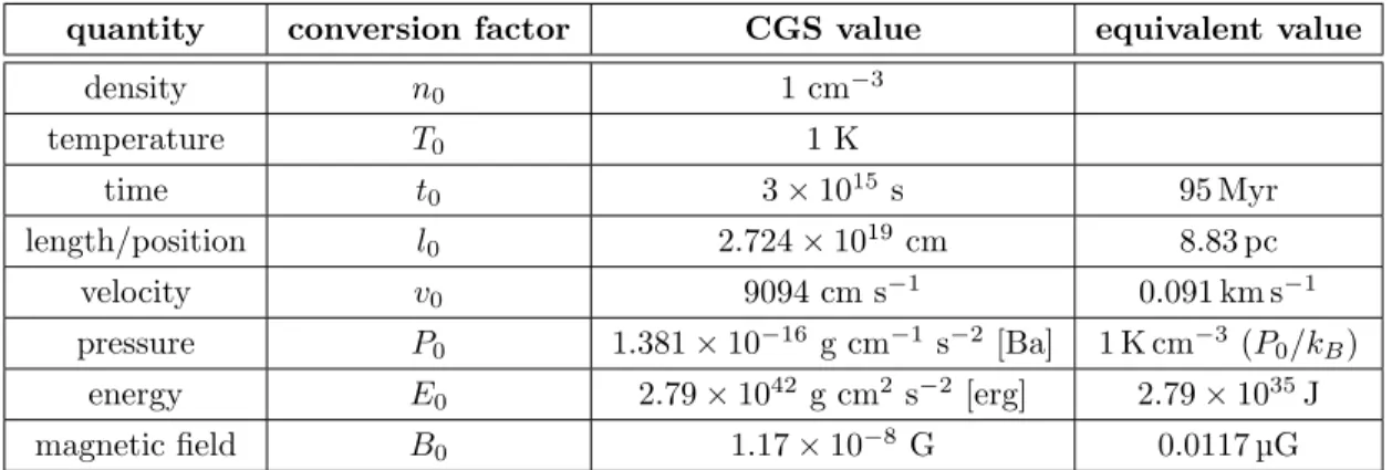
I determine the initial densities and pressure from Figure 2, which shows pressure as a function of density at thermal equilibrium, as given by the heating and cooling model functions (Sec. 1.2). Based on this plot, I select initial densities that can coexist at the same equilibrium pressure. I select a halo densityρh= 0.316
and a cloud density ρc = 28.265, with a uniform pressureP = 2113.65 throughout the simulation domain,
as required for thermal equilibrium.
2.2.2 Boundary Conditions
I use periodic boundary conditions at the x-boundaries (three dimensions: x- and y-) of the simulation domain. Inflow of hot, diffuse gas occurs at the lowery-boundary (three dimensions: z-), with an upwards inflow velocity ofvh, as given in Sec. 2.2.1. The upper boundary allows for inflow of cold, dense gas, with a
downwards velocity ofvc.
The boundary cells are subject to the same corrections of velocity and other quantities, as required for the comoving reference frame (Sec. 2.1.3).
2.2.3 Scalar Fields
Each simulation contains three passive scalar fields, which I use as tracers. At any given point in the domain, the value of a scalar fieldS can be calculated from the densityρand the colorcof the field:
S0marks the interface between the cloud and the halo. It is initialized as a Gaussian distribution around
the interface, with a standard deviation of 0.05 (= 0.44 pc) and a peak color value c0= 1 at the calculated
interface position.
S1 is used to trace the cloud gas. It is initialized withc1= 1 in the dense cloud gas and c1 = 0 in the
diffuse halo gas.
S2traces the inflow of gas that enters the simulation domain at the lower boundary iny(three dimensions:
z) and flows upward toward the halo-cloud interface. All gas initially within the simulation domain, as well as gas in the ghost cells at the upper boundary, receives a color c2= 0. Only gas flowing in from the lower
boundary is givenc2= 1.
2.2.4 Magnetic Fields
For the RTI driven by ram pressure, the critical field strength (Eq. 37) can be written as
Bc =
Lρv
2
Σ (ρ2−ρ1) 1/2
=
LM
2P 1
Σ (ρ2−ρ1) 1/2
, (62)
whereP1is the thermal pressure in the diffuse gas andMis the Mach number of the inflow. Alternatively,
Bc can be expressed as the critical ratio between thermal and magnetic pressure, or the plasmaβ,
βc =
8πPtherm
B2
c
= 25 κ
M2 (63)
for the specific simulation parameters used. Here,κis the number of wave modes in the interface.
For the 2D models, I explore a sequence of plasma β, from βc/2 to 32βc, to highlight the difference
between the ram pressure- and gravity-driven magnetized RTI. The domain is initialized with a constant magnetic field in thex-direction.
2.3
Heating and Cooling
I use Athena’s third-order Runge-Kutta (RK3) method to integrate Equations 38-41. Within the RK3 integrator, safeguards are established to prevent non-physical results: if the internal energy or the density becomes negative, the RK3 algorithm will retry the integration up to five times, halving the timestep for each attempt.
Heating and cooling are implemented as a source term in the total energy equation (Eq. 40) through subcycling: the radiative losses are applied via an embedded Runge-Kutta-Fehlberg (RK45) algorithm within the RK3 substeps. The RK45 integrator uses an adaptive step size and contains safeguards to guarantee a positive temperature and limit the temperature change of each RK45 step. Subcycling is necessary since the cooling timescale is usually at least one order of magnitude shorter than the timestep imposed by the Courant-Friedrichs-Lewy stability condition.
2.4
Definitions
Here, I briefly discuss two measures used to quantify and analyze the simulation results: the interface amplitude as a measure for the instability growth (Sec. 2.4.1), and the mixing length as a measure for mixing between the cloud and halo gas (Sec. 2.4.2).
2.4.1 Amplitude
The amplitude Ais given by
A=
P
i,j(y[i, j]− hyi)
2
·S0[i, j]
P
i,jS0[i, j]
!1/2
, (64)
where the scalar-weighted meany-positionhyiis
hyi= P
i,jy[i, j]·S0[i, j]
P
i,jS0[i, j]
. (65)
2.4.2 Mixing Length
The measurement of mixing length is based on the work of Cook et al. (2004) and Cabot & Cook (2006), as summarized by Zhou (2017). I modify their approach to use the color of the passive scalar field S1,
initialized with color c1 = 1 in the cloud gas and c1 = 0 in the halo gas, accounting for the case of
non-reacting and incompressible gases in my simulations. The mole fractionX of the dense (cloud) gas at any point within the simulation domain is given by
X = c−ch
cc+ch
, (66)
wherecc andchare the respective colors of the cloud and halo gas, andcis the color of the scalar fieldS1at
that point. The mole fractionXP of perfectly mixed gas (consisting of halo and cloud gas in equal parts) is
XP(X) =
(
2X ifX≤1/2
2(1−X) ifX >1/2
= 2 min(X,1−X). (67)
The mixing lengthhis then calculated as follows:
h=
Z y2
y1
XP(hXi)dy, (68)
wherey1andy2 are the lower and upper boundaries of the simulation domain in the two-dimensional case.
(In three dimensions,his determined by taking this integral fromz1to z2with respect to z.)
If the halo and cloud gas were perfectly mixed in x(three dimensions: inxand y), this mixing length would be the height of the corresponding layer of mixed gas (Cook et al. 2004; Cabot & Cook 2006).
3
Results
I will start by assessing the impact of numerical resolution on the simulation results (Sec. 3.1), using the two-dimensional simulations. The three-dimensional RTI is explored in Sec. 3.2, and I discuss the effects of magnetic fields in Sec. 3.3.
3.1
Resolution Study in Two Dimensions
0.50 0.25 0.00 0.25 0.50 x
1.00 0.75 0.50 0.25 0.00 0.25 0.50 0.75 1.00
y
0.50 0.25 0.00 0.25 0.50 0.75 1.00 1.25
log d
0
1
log d
1.00
0.75
0.50
0.25
0.00
0.25
0.50
0.75
1.00
y
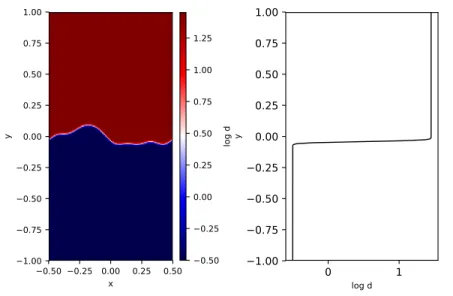
Figure 3: Logarithm of the gas density att= 0 for the two-dimensional RTI. Map is shown on the left, and a profile taken along they-direction atx= 0 is shown on the right.
3.1.1 Adiabatic Models
Figure 3 shows the initial density profile for the two-dimensional RTI. This same perturbation shape and strength is used for the initialization of each run.
Figure 4 contains snapshots of the density (d) for each of the four test resolutions: N128, N256, N512, and N1024. In the adiabatic case, the initial shock from the halo gas quickly affects the cloud gas. The transition region between the fluids expands toward the upper boundary. Att= 0.05, the interface remains within the grid, but byt= 0.1 it has reached the y-boundaries, leaving only halo gas and the mixing region behind. Byt= 0.4, the grid is filled with turbulent mixing of the halo and cloud gas. Since the perturbations are now limited by the imposed boundary values, the results cannot be used for physical interpretation at this time. The effect of the boundaries can be seen for N128 in Fig. 4 (bottom left) as a thin blue region at the bottom.
Additionally, careful inspection of the plots in Figure 4 reveals the effects of resolution. Higher resolutions provide finer detail and show evolution on smaller scales. Moreover, although they are generally similar, the density profiles appear slightly different at each resolution. To evaluate the impact of these small discrepancies, I compare the amplitude A (Eq. 64) and the mixing length h(Eq. 68) of the instability in each run. Figure 5a shows the amplitude plotted against time, and Figure 5b shows the mixing length. The linear growth phase untilt= 0.05 is nearly independent of resolution, yet, once secondary instabilities and eventually turbulence develop, the models start to differ. Figure 5a shows that N128 diverges slightly from the others, but N256, N512, and N1024 are in close agreement until t ∼0.1, by which point the interface has reached the upper and lower boundaries. Similarly, the time evolution of the mixing lengths is roughly the same at each resolution untilt∼0.1.
3.1.2 Radiative Models
For runs including radiative losses (heating and cooling), the interface perturbation has the same shape as in the adiabatic case, as shown in Figure 3.
0.50 0.25 0.00 0.25 0.50 x 1.00 0.75 0.50 0.25 0.00 0.25 0.50 0.75 y 0.00 0.25 0.50 0.75 1.00 1.25 1.50 1.75 log d
0 1 2
log d 1.00 0.75 0.50 0.25 0.00 0.25 0.50 0.75 y
0.50 0.25 0.00 0.25 0.50 x 1.00 0.75 0.50 0.25 0.00 0.25 0.50 0.75 y 0.00 0.25 0.50 0.75 1.00 1.25 1.50 1.75 log d
0 1 2
log d 1.00 0.75 0.50 0.25 0.00 0.25 0.50 0.75 y
0.50 0.25 0.00 0.25 0.50 x 1.00 0.75 0.50 0.25 0.00 0.25 0.50 0.75 y 0.00 0.25 0.50 0.75 1.00 1.25 1.50 1.75 log d
0 1 2
log d 1.00 0.75 0.50 0.25 0.00 0.25 0.50 0.75 y
0.50 0.25 0.00 0.25 0.50 x 1.00 0.75 0.50 0.25 0.00 0.25 0.50 0.75 y 0.00 0.25 0.50 0.75 1.00 1.25 1.50 1.75 log d
0 1 2
log d 1.00 0.75 0.50 0.25 0.00 0.25 0.50 0.75 y
0.50 0.25 0.00 0.25 0.50 x 1.00 0.75 0.50 0.25 0.00 0.25 0.50 0.75 y 0.00 0.25 0.50 0.75 1.00 1.25 1.50 1.75 log d 0 1 log d 1.00 0.75 0.50 0.25 0.00 0.25 0.50 0.75 y
0.50 0.25 0.00 0.25 0.50 x 1.00 0.75 0.50 0.25 0.00 0.25 0.50 0.75 y 0.00 0.25 0.50 0.75 1.00 1.25 1.50 1.75 log d
0 1 2 log d 1.00 0.75 0.50 0.25 0.00 0.25 0.50 0.75 y
0.50 0.25 0.00 0.25 0.50 x 1.25 1.00 0.75 0.50 0.25 0.00 0.25 0.50 y 0.00 0.25 0.50 0.75 1.00 1.25 1.50 1.75 log d
0 1 2
log d 1.25 1.00 0.75 0.50 0.25 0.00 0.25 0.50 y
0.50 0.25 0.00 0.25 0.50 x 1.25 1.00 0.75 0.50 0.25 0.00 0.25 0.50 y 0.00 0.25 0.50 0.75 1.00 1.25 1.50 1.75 log d
0 1 2
log d 1.25 1.00 0.75 0.50 0.25 0.00 0.25 0.50 y
0.50 0.25 0.00 0.25 0.50 x 1.25 1.00 0.75 0.50 0.25 0.00 0.25 0.50 y 0.00 0.25 0.50 0.75 1.00 1.25 1.50 1.75 log d 0 1 log d 1.25 1.00 0.75 0.50 0.25 0.00 0.25 0.50 y
0.50 0.25 0.00 0.25 0.50 x 1.50 1.25 1.00 0.75 0.50 0.25 0.00 0.25 y 0.00 0.25 0.50 0.75 1.00 1.25 1.50 1.75 log d 0 1 log d 1.50 1.25 1.00 0.75 0.50 0.25 0.00 0.25 y
0.50 0.25 0.00 0.25 0.50 x 1.75 1.50 1.25 1.00 0.75 0.50 0.25 0.00 y 0.00 0.25 0.50 0.75 1.00 1.25 1.50 1.75 log d 0 1 log d 1.75 1.50 1.25 1.00 0.75 0.50 0.25 0.00 y
0.50 0.25 0.00 0.25 0.50 x 1.75 1.50 1.25 1.00 0.75 0.50 0.25 0.00 y 0.00 0.25 0.50 0.75 1.00 1.25 1.50 1.75 log d 0 1 log d 1.75 1.50 1.25 1.00 0.75 0.50 0.25 0.00 y
0.0 0.1 0.2 0.3 0.4 0.5 time
0.1 0.2 0.3 0.4 0.5 0.6
amp
n128 n256 n512 n1024
(a) Amplitude vs. time.
0.0 0.1 0.2 0.3 0.4 0.5 time
0.2 0.4 0.6 0.8 1.0 1.2 1.4
mix-len
n128 n256 n512 n1024
(b) Mixing length vs. time.
Figure 5: Amplitude and mixing length vs. time for the adiabatic instability in 2D (N128, N256, N512, and N1024). The linear growth phase until t ∼ 0.05 is nearly independent of resolution. The results slightly diverge once turbulence develops.
the simulation domain, allowing for a longer time span to follow the evolution of the instability.
The effects of resolution can be observed in Figure 6 as well. As in the adiabatic case, higher resolution yields finer detail and shows the small-scale evolution of the instability. Additionally, the density profiles at each resolution show small differences despite their general similarity in shape and size.
Figure 7 shows the amplitude and mixing length plotted against time for each of the four test resolutions. The amplitudes (Fig. 7a) are similar untilt∼0.1, at which point the runs diverge. For the mixing lengths (Fig. 7b), the similarity lasts untilt∼0.15. The mixing lengths then begin to decrease, suggesting that the instability reaches saturation around that time. Amplitude and mixing length generally appear to increase with higher resolution; however, N512 shows fluctuations not observed at other resolutions—a noticeable decrease in amplitude while that quantity increased in other runs, as well as a sharper decline in mixing length.
3.2
The Three-Dimensional RTI
In three dimensions, the simulation domain is of sizeL×L×2L, with L= 1.0 = 8.8 pc, corresponding with a computational grid of sizeN ×N×2N cells for a given resolutionN. I explore both the adiabatic and radiative versions of the instability at resolutions N128 and N256.
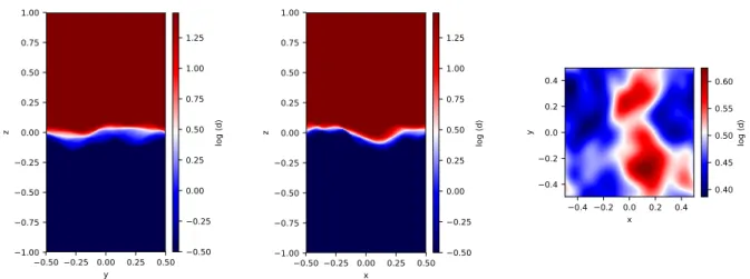
The initial density profile for the three-dimensional RTI is shown in Figure 8. This perturbation shape and strength is used for all 3D runs.
Figure 9 shows the evolution of the instability for the adiabatic and radiative cases. Snapshots of the mean density along thex-direction are shown fort= 0.05, 0.1, and 0.4. As in the two-dimensional runs, the interface quickly reaches the lower and upper boundaries in the adiabatic version. When heating and cooling are included, the interface remains within the grid, providing a more meaningful look at the instability and its evolution. The two resolutions N128 and N256 produce generally similar results.
0.50 0.25 0.00 0.25 0.50 x 0.75 0.50 0.25 0.00 0.25 0.50 0.75 1.00 y 0.5 0.0 0.5 1.0 1.5 2.0 2.5 log d
0 1 2 3 log d 0.75 0.50 0.25 0.00 0.25 0.50 0.75 1.00 y
0.50 0.25 0.00 0.25 0.50 x 1.00 0.75 0.50 0.25 0.00 0.25 0.50 0.75 y 0.5 0.0 0.5 1.0 1.5 2.0 2.5 log d
0 1 2 3 log d 1.00 0.75 0.50 0.25 0.00 0.25 0.50 0.75 y
0.50 0.25 0.00 0.25 0.50 x 1.00 0.75 0.50 0.25 0.00 0.25 0.50 0.75 y 0.5 0.0 0.5 1.0 1.5 2.0 2.5 3.0 log d
0 1 2 3 log d 1.00 0.75 0.50 0.25 0.00 0.25 0.50 0.75 y
0.50 0.25 0.00 0.25 0.50 x 1.00 0.75 0.50 0.25 0.00 0.25 0.50 0.75 y 0.5 0.0 0.5 1.0 1.5 2.0 2.5 3.0 log d 0 2 log d 1.00 0.75 0.50 0.25 0.00 0.25 0.50 0.75 y
0.50 0.25 0.00 0.25 0.50 x 0.75 0.50 0.25 0.00 0.25 0.50 0.75 1.00 y 0.0 0.5 1.0 1.5 2.0 2.5 3.0 log d
0 1 2 3
log d 0.75 0.50 0.25 0.00 0.25 0.50 0.75 1.00 y
0.50 0.25 0.00 0.25 0.50 x 0.75 0.50 0.25 0.00 0.25 0.50 0.75 1.00 y 0.5 0.0 0.5 1.0 1.5 2.0 2.5 3.0 log d
0 1 2 3 log d 0.75 0.50 0.25 0.00 0.25 0.50 0.75 1.00 y
0.50 0.25 0.00 0.25 0.50 x 1.00 0.75 0.50 0.25 0.00 0.25 0.50 0.75 y 0.5 0.0 0.5 1.0 1.5 2.0 2.5 3.0 log d
0 1 2 3 log d 1.00 0.75 0.50 0.25 0.00 0.25 0.50 0.75 y
0.50 0.25 0.00 0.25 0.50 x 1.00 0.75 0.50 0.25 0.00 0.25 0.50 0.75 y 0.5 0.0 0.5 1.0 1.5 2.0 2.5 3.0 log d 0 2 log d 1.00 0.75 0.50 0.25 0.00 0.25 0.50 0.75 y
0.50 0.25 0.00 0.25 0.50 x 0.75 0.50 0.25 0.00 0.25 0.50 0.75 1.00 y 0.0 0.5 1.0 1.5 2.0 2.5 log d
0 1 2 3
log d 0.75 0.50 0.25 0.00 0.25 0.50 0.75 1.00 y
0.50 0.25 0.00 0.25 0.50 x 1.00 0.75 0.50 0.25 0.00 0.25 0.50 0.75 y 0.0 0.5 1.0 1.5 2.0 2.5 log d
0 1 2 3
log d 1.00 0.75 0.50 0.25 0.00 0.25 0.50 0.75 y
0.50 0.25 0.00 0.25 0.50 x 1.00 0.75 0.50 0.25 0.00 0.25 0.50 0.75 y 0.0 0.5 1.0 1.5 2.0 2.5 3.0 log d
0 1 2 3
log d 1.00 0.75 0.50 0.25 0.00 0.25 0.50 0.75 y
0.50 0.25 0.00 0.25 0.50 x 0.75 0.50 0.25 0.00 0.25 0.50 0.75 1.00 y 0.0 0.5 1.0 1.5 2.0 2.5 3.0 log d
0 1 2 3
log d 0.75 0.50 0.25 0.00 0.25 0.50 0.75 1.00 y
0.0 0.1 0.2 0.3 0.4 0.5 time
0.05 0.10 0.15 0.20 0.25 0.30 0.35 0.40
amp
n128 n256 n512 n1024
(a) Amplitude vs. time.
0.0 0.1 0.2 0.3 0.4 0.5 time
0.10 0.15 0.20 0.25 0.30 0.35 0.40 0.45
mix-len
n128 n256 n512 n1024
(b) Mixing length vs. time.
Figure 7: Amplitude and mixing length vs. time for the instability in 2D with radiative losses (N128, N256, N512, and N1024). Growth is relatively independent of resolution until t∼0.1 for amplitude andt∼0.15 for mixing length.
0.50 0.25 0.00 0.25 0.50 y
1.00 0.75 0.50 0.25 0.00 0.25 0.50 0.75 1.00
z
0.50 0.25 0.00 0.25 0.50 0.75 1.00 1.25
log
d
0 1
log d
1.00 0.75 0.50 0.25 0.00 0.25 0.50 0.75 1.00
z
0.50 0.25 0.00 0.25 0.50 x
1.00 0.75 0.50 0.25 0.00 0.25 0.50 0.75 1.00
z
0.50 0.25 0.00 0.25 0.50 0.75 1.00 1.25
log
d
0 1
log d 1.00
0.75 0.50 0.25 0.00 0.25 0.50 0.75 1.00
z
0.4 0.2 0.0 0.2 0.4 x
0.4 0.2 0.0 0.2 0.4
y
0.40 0.45 0.50 0.55 0.60
log
d
0.4 0.5 0.6
log d
0.4 0.2 0.0 0.2 0.4
y
Figure 8: Initial density profile for the three-dimensional RTI. Left to right: views along the x-, y-, and
0.50 0.25 0.00 0.25 0.50 y 1.00 0.75 0.50 0.25 0.00 0.25 0.50 0.75 z 0.00 0.25 0.50 0.75 1.00 1.25 1.50 1.75 log d 0 1
log d 1.00 0.75 0.50 0.25 0.00 0.25 0.50 0.75 z
0.50 0.25 0.00 0.25 0.50 y 1.00 0.75 0.50 0.25 0.00 0.25 0.50 0.75 z 0.00 0.25 0.50 0.75 1.00 1.25 1.50 1.75 log d 0 1
log d 1.00 0.75 0.50 0.25 0.00 0.25 0.50 0.75 z
0.50 0.25 0.00 0.25 0.50 y 0.75 0.50 0.25 0.00 0.25 0.50 0.75 1.00 z 0.5 0.0 0.5 1.0 1.5 2.0 log d
0 1 2 log d 0.75 0.50 0.25 0.00 0.25 0.50 0.75 1.00 z
0.50 0.25 0.00 0.25 0.50 y 1.00 0.75 0.50 0.25 0.00 0.25 0.50 0.75 z 0.5 0.0 0.5 1.0 1.5 2.0 log d
0 1 2
log d 1.00 0.75 0.50 0.25 0.00 0.25 0.50 0.75 z
0.50 0.25 0.00 0.25 0.50 y 1.00 0.75 0.50 0.25 0.00 0.25 0.50 0.75 z 0.00 0.25 0.50 0.75 1.00 1.25 1.50 1.75 log d 0 1
log d 1.00 0.75 0.50 0.25 0.00 0.25 0.50 0.75 z
0.50 0.25 0.00 0.25 0.50 y 1.25 1.00 0.75 0.50 0.25 0.00 0.25 0.50 z 0.00 0.25 0.50 0.75 1.00 1.25 1.50 1.75 log d 0 1
log d 1.25 1.00 0.75 0.50 0.25 0.00 0.25 0.50 z
0.50 0.25 0.00 0.25 0.50 y 0.75 0.50 0.25 0.00 0.25 0.50 0.75 1.00 z 0.5 0.0 0.5 1.0 1.5 2.0 log d
0 1 2
log d 0.75 0.50 0.25 0.00 0.25 0.50 0.75 1.00 z
0.50 0.25 0.00 0.25 0.50 y 1.00 0.75 0.50 0.25 0.00 0.25 0.50 0.75 z 0.5 0.0 0.5 1.0 1.5 2.0 log d
0 1 2
log d 1.00 0.75 0.50 0.25 0.00 0.25 0.50 0.75 z
0.50 0.25 0.00 0.25 0.50 y 1.25 1.00 0.75 0.50 0.25 0.00 0.25 0.50 z 0.00 0.25 0.50 0.75 1.00 1.25 1.50 1.75 log d 0 1
log d 1.25 1.00 0.75 0.50 0.25 0.00 0.25 0.50 z
0.50 0.25 0.00 0.25 0.50 y 1.50 1.25 1.00 0.75 0.50 0.25 0.00 0.25 z 0.00 0.25 0.50 0.75 1.00 1.25 1.50 1.75 log d 0 1
log d 1.50 1.25 1.00 0.75 0.50 0.25 0.00 0.25 z
0.50 0.25 0.00 0.25 0.50 y 1.00 0.75 0.50 0.25 0.00 0.25 0.50 0.75 z 0.0 0.5 1.0 1.5 2.0 2.5 log d
0 1 2
log d 1.00 0.75 0.50 0.25 0.00 0.25 0.50 0.75 z
0.50 0.25 0.00 0.25 0.50 y 1.00 0.75 0.50 0.25 0.00 0.25 0.50 0.75 z 0.0 0.5 1.0 1.5 2.0 log d
0 1 2
log d 1.00 0.75 0.50 0.25 0.00 0.25 0.50 0.75 z
0.00 0.05 0.10 0.15 0.20 0.25 0.30 0.35 0.40 time
0.1 0.2 0.3 0.4 0.5
amp
n128ad n256ad n128 n256
(a) Amplitude vs. time.
0.00 0.05 0.10 0.15 0.20 0.25 0.30 0.35 0.40 time
0.2 0.4 0.6 0.8 1.0 1.2
mix-len
n128ad n256ad n128 n256
(b) Mixing length vs. time.
Figure 10: Amplitude and mixing length vs. time for the instability in 3D. Both adiabatic (“ad”) and radiative runs are shown. Cooling keeps the interface more compressed, slowing the instability growth.
3.3
Magnetic Fields
I assess the effects of magnetic fields on the RTI in two and three dimensions. I also test both adiabatic and radiative models to evaluate the combined impact of cooling and magnetic fields.
3.3.1 Magnetic Fields in Two Dimensions
Magnetic fields aligned with the interface can suppress the RTI in two dimensions by providing an effective surface tension (Sec. 2.2.4). Since the gravitational acceleration is replaced by an acceleration term proportional to the ram pressure, the resulting critical field strength will scale with the Mach number of the inflow,M(Eq. 37).
Yet Figure 11a suggests that the estimate for the critical field strength is not correct. Starting at half the critical plasmaβc and running up all the way to 32βc, the instability progressively develops, but never
reaches the hydrodynamical (B= 0) amplitude. Figure 12 provides a more detailed view. The top row shows snapshots of the density field att= 0.05 for the adiabatic runs, with the plasmaβincreasing from left to right (i.e., the magnetic field gets weaker from left to right). At the highest field strength (lowestβ), the interface develops a sinusoidal shape facing the low-density gas. The magnetic tension component of the Lorentz force counterbalances the ram pressure imbalance, and the perturbation amplitudes eventually decrease with time (see also Fig. 11a). With decreasing field strength, two effects occur. The perturbations become more pronounced, consistent with the critical field strength argument, and perturbations at higher wavenumbers start to grow, which is expected from the scale-dependency of the critical field strength (Eq. 37).
The situation is more extreme for the cooling runs (Fig. 11b and bottom row of Fig. 12). Even a small magnetic field suppresses instability growth, yet the same tendency as for the adiabatic sequence can be observed: with decreasing field strength, the amplitudes tend to grow. The main difference from the adiabatic models is the radiative losses, increasing the density in the cloud gas. The density (and thus the magnetic field) increase can be roughly estimated by balancing the pressures, assuming that the cloud gas is initially at rest, and that the magnetic pressure is negligible compared to the thermal and ram pressure:
ρc=
1
c2
c
P+ρhv2h
, (69)
0.00 0.05 0.10 0.15 0.20 0.25 0.30 0.35 0.40 time
0.0 0.1 0.2 0.3 0.4 0.5
amp
2DH 2DM32 2DM16 2DM8 2DM4 2DM2 2DM0.5
(a) Adiabatic MHD models.
0.00 0.05 0.10 0.15 0.20 0.25 0.30 0.35 0.40 time
0.00 0.05 0.10 0.15 0.20
amp
2DH 2DM32 2DM16 2DM8 2DM4 2DM2 2DM0.5
(b) MHD models with cooling.
Figure 11: Amplitude of the interface layer (Eq. 64) against time. For the adiabatic case, the instability should grow forβ > βc, but it only fully develops for β >16βc. No instability growth is observed for the
cooling case.
3.3.2 Magnetic Fields in Three Dimensions
As shown by Chandrasekhar (Sec. 1.3), a magnetic field parallel to the interface between the halo and cloud gas should have no impact on modes perpendicular to B~, while modes parallel to B~ are suppressed for fieldsB > Bc, whereBc is the critical field strength given by Eq. 62. Therefore, while growth along the
x-direction was suppressed in 2D runs, for 3D runs some growth along they-direction can be expected. Figure 13 compares the evolution of the instability (including radiative losses) with and without a mag-netic field in two and three dimensions. The magmag-netic field does suppress the growth of the instability in two dimensions (as shown also in Sec. 3.3.1). In three dimensions, however, the instability grows in the presence of magnetic fields. Applying a magnetic field results in a more clearly defined interface, as well as the growth of large “fingers” downwards. The top of the interface remains relatively flat and reaches the upper boundary of the grid byt= 0.2.
Figure 14 contains snapshots of the density att= 0.0, 0.05, and 0.1. The views along thez-axis show that variations in thex-direction are smoothed away as time passes, leaving perturbations along they-direction. This development matches the theoretical expectations for the magnetic field in thex-direction.
4
Discussion
Not only magnetic fields, but also radiative losses, can strongly affect the evolution of the RTI. While magnetic fields give rise to an effective surface tension and thus introduce anisotropy in three dimensions, leading eventually to super-hydrodynamical growth rates, radiative losses result in rapid mass accumulation and eventually fragmentation of the initial (large-scale) instability modes. Combining magnetic fields and radiative losses in three dimensions recovers the instability.
4.1
Heating and Cooling Effects
0.50 0.25 0.00 0.25 0.50 x 0.75 0.50 0.25 0.00 0.25 0.50 0.75 1.00 y 0.00 0.25 0.50 0.75 1.00 1.25 1.50 1.75 log d
0 1 2
log d 0.75 0.50 0.25 0.00 0.25 0.50 0.75 1.00 y
0.50 0.25 0.00 0.25 0.50 x 0.75 0.50 0.25 0.00 0.25 0.50 0.75 1.00 y 0.00 0.25 0.50 0.75 1.00 1.25 1.50 1.75 log d
0 1 2
log d 0.75 0.50 0.25 0.00 0.25 0.50 0.75 1.00 y
0.50 0.25 0.00 0.25 0.50 x 0.75 0.50 0.25 0.00 0.25 0.50 0.75 1.00 y 0.00 0.25 0.50 0.75 1.00 1.25 1.50 1.75 log d
0 1 2
log d 0.75 0.50 0.25 0.00 0.25 0.50 0.75 1.00 y
0.50 0.25 0.00 0.25 0.50 x 0.75 0.50 0.25 0.00 0.25 0.50 0.75 1.00 y 0.00 0.25 0.50 0.75 1.00 1.25 1.50 1.75 log d
0 1 2
log d 0.75 0.50 0.25 0.00 0.25 0.50 0.75 1.00 y
0.50 0.25 0.00 0.25 0.50 x 0.75 0.50 0.25 0.00 0.25 0.50 0.75 1.00 y 0.00 0.25 0.50 0.75 1.00 1.25 1.50 1.75 log d
0 1 2
log d 0.75 0.50 0.25 0.00 0.25 0.50 0.75 1.00 y
0.50 0.25 0.00 0.25 0.50 x 0.75 0.50 0.25 0.00 0.25 0.50 0.75 1.00 y 0.00 0.25 0.50 0.75 1.00 1.25 1.50 1.75 2.00 log d
0 1 2
log d 0.75 0.50 0.25 0.00 0.25 0.50 0.75 1.00 y
0.50 0.25 0.00 0.25 0.50 x 0.75 0.50 0.25 0.00 0.25 0.50 0.75 1.00 y 0.0 0.5 1.0 1.5 2.0 2.5 log d
0 1 2
log d 0.75 0.50 0.25 0.00 0.25 0.50 0.75 1.00 y
0.50 0.25 0.00 0.25 0.50 x 0.75 0.50 0.25 0.00 0.25 0.50 0.75 1.00 y 0.0 0.5 1.0 1.5 2.0 2.5 log d
0 1 2 3
log d 0.75 0.50 0.25 0.00 0.25 0.50 0.75 1.00 y
0.50 0.25 0.00 0.25 0.50 x 0.75 0.50 0.25 0.00 0.25 0.50 0.75 1.00 y 0.0 0.5 1.0 1.5 2.0 2.5 log d
0 1 2 3
log d 0.75 0.50 0.25 0.00 0.25 0.50 0.75 1.00 y
0.50 0.25 0.00 0.25 0.50 x 0.75 0.50 0.25 0.00 0.25 0.50 0.75 1.00 y 0.0 0.5 1.0 1.5 2.0 2.5 log d
0 1 2 3
log d 0.75 0.50 0.25 0.00 0.25 0.50 0.75 1.00 y
0.50 0.25 0.00 0.25 0.50 x 0.75 0.50 0.25 0.00 0.25 0.50 0.75 1.00 y 0.5 0.0 0.5 1.0 1.5 2.0 2.5 3.0 log d
0 1 2 3
log d 0.75 0.50 0.25 0.00 0.25 0.50 0.75 1.00 y
0.50 0.25 0.00 0.25 0.50 x 0.75 0.50 0.25 0.00 0.25 0.50 0.75 1.00 y 0.5 0.0 0.5 1.0 1.5 2.0 2.5 3.0 log d
0 1 2 3
log d 0.75 0.50 0.25 0.00 0.25 0.50 0.75 1.00 y
0.50 0.25 0.00 0.25 0.50 x 0.50 0.25 0.00 0.25 0.50 0.75 1.00 1.25 y 0.00 0.25 0.50 0.75 1.00 1.25 1.50 1.75 log d
0 1 2
log d 0.50 0.25 0.00 0.25 0.50 0.75 1.00 1.25 y
0.50 0.25 0.00 0.25 0.50 x 0.50 0.25 0.00 0.25 0.50 0.75 1.00 1.25 y 0.00 0.25 0.50 0.75 1.00 1.25 1.50 1.75 log d
0 1 2
log d 0.50 0.25 0.00 0.25 0.50 0.75 1.00 1.25 y
0.50 0.25 0.00 0.25 0.50 x 0.50 0.25 0.00 0.25 0.50 0.75 1.00 1.25 y 0.00 0.25 0.50 0.75 1.00 1.25 1.50 1.75 log d
0 1 2
log d 0.50 0.25 0.00 0.25 0.50 0.75 1.00 1.25 y
0.50 0.25 0.00 0.25 0.50 x 0.75 0.50 0.25 0.00 0.25 0.50 0.75 1.00 y 0.00 0.25 0.50 0.75 1.00 1.25 1.50 1.75 log d
0 1 2
log d 0.75 0.50 0.25 0.00 0.25 0.50 0.75 1.00 y
0.50 0.25 0.00 0.25 0.50 x 0.75 0.50 0.25 0.00 0.25 0.50 0.75 1.00 y 0.00 0.25 0.50 0.75 1.00 1.25 1.50 1.75 log d
0 1 2
log d 0.75 0.50 0.25 0.00 0.25 0.50 0.75 1.00 y
0.50 0.25 0.00 0.25 0.50 x 0.75 0.50 0.25 0.00 0.25 0.50 0.75 1.00 y 0.00 0.25 0.50 0.75 1.00 1.25 1.50 1.75 log d
0 1 2
log d 0.75 0.50 0.25 0.00 0.25 0.50 0.75 1.00 y
0.50 0.25 0.00 0.25 0.50 x 0.75 0.50 0.25 0.00 0.25 0.50 0.75 1.00 y 0.0 0.5 1.0 1.5 2.0 log d
0 1 2
log d 0.75 0.50 0.25 0.00 0.25 0.50 0.75 1.00 y
0.50 0.25 0.00 0.25 0.50 x 0.75 0.50 0.25 0.00 0.25 0.50 0.75 1.00 y 0.0 0.5 1.0 1.5 2.0 2.5 log d
0 1 2
log d 0.75 0.50 0.25 0.00 0.25 0.50 0.75 1.00 y
0.50 0.25 0.00 0.25 0.50 x 0.75 0.50 0.25 0.00 0.25 0.50 0.75 1.00 y 0.0 0.5 1.0 1.5 2.0 2.5 log d
0 1 2
log d 0.75 0.50 0.25 0.00 0.25 0.50 0.75 1.00 y
0.50 0.25 0.00 0.25 0.50 x 0.75 0.50 0.25 0.00 0.25 0.50 0.75 1.00 y 0.0 0.5 1.0 1.5 2.0 2.5 log d
0 1 2
log d 0.75 0.50 0.25 0.00 0.25 0.50 0.75 1.00 y
0.50 0.25 0.00 0.25 0.50 x 0.75 0.50 0.25 0.00 0.25 0.50 0.75 1.00 y 0.0 0.5 1.0 1.5 2.0 2.5 log d
0 1 2
log d 0.75 0.50 0.25 0.00 0.25 0.50 0.75 1.00 y
0.50 0.25 0.00 0.25 0.50 x 0.75 0.50 0.25 0.00 0.25 0.50 0.75 1.00 y 0.0 0.5 1.0 1.5 2.0 2.5 log d
0 1 2
log d 0.75 0.50 0.25 0.00 0.25 0.50 0.75 1.00 y
0.50 0.25 0.00 0.25 0.50 x 0.75 0.50 0.25 0.00 0.25 0.50 0.75 1.00 y 0.5 0.0 0.5 1.0 1.5 2.0 2.5 log d
0 1 2 3 log d 0.75 0.50 0.25 0.00 0.25 0.50 0.75 1.00 y
0.50 0.25 0.00 0.25 0.50 x 0.75 0.50 0.25 0.00 0.25 0.50 0.75 1.00 y 0.0 0.5 1.0 1.5 2.0 2.5 log d
0 1 2
log d 0.75 0.50 0.25 0.00 0.25 0.50 0.75 1.00 y
0.50 0.25 0.00 0.25 0.50 y 0.75 0.50 0.25 0.00 0.25 0.50 0.75 1.00 z 0.5 0.0 0.5 1.0 1.5 2.0 log d
0 1 2 log d 0.75 0.50 0.25 0.00 0.25 0.50 0.75 1.00 z
0.50 0.25 0.00 0.25 0.50 y 0.75 0.50 0.25 0.00 0.25 0.50 0.75 1.00 z 0.0 0.5 1.0 1.5 2.0 log d
0 1 2
log d 0.75 0.50 0.25 0.00 0.25 0.50 0.75 1.00 z
0.50 0.25 0.00 0.25 0.50 x 0.75 0.50 0.25 0.00 0.25 0.50 0.75 1.00 y 0.0 0.5 1.0 1.5 2.0 2.5 3.0 log d
0 1 2 3
log d 0.75 0.50 0.25 0.00 0.25 0.50 0.75 1.00 y
0.50 0.25 0.00 0.25 0.50 x 0.75 0.50 0.25 0.00 0.25 0.50 0.75 1.00 y 0.0 0.5 1.0 1.5 2.0 log d
0 1 2
log d 0.75 0.50 0.25 0.00 0.25 0.50 0.75 1.00 y
0.50 0.25 0.00 0.25 0.50 y 0.75 0.50 0.25 0.00 0.25 0.50 0.75 1.00 z 0.5 0.0 0.5 1.0 1.5 2.0 log d
0 1 2
log d 0.75 0.50 0.25 0.00 0.25 0.50 0.75 1.00 z
0.50 0.25 0.00 0.25 0.50 y 0.75 0.50 0.25 0.00 0.25 0.50 0.75 1.00 z 0.0 0.5 1.0 1.5 2.0 log d
0 1 2
log d 0.75 0.50 0.25 0.00 0.25 0.50 0.75 1.00 z
0.50 0.25 0.00 0.25 0.50 x 0.75 0.50 0.25 0.00 0.25 0.50 0.75 1.00 y 0.0 0.5 1.0 1.5 2.0 2.5 3.0 log d
0 1 2 3
log d 0.75 0.50 0.25 0.00 0.25 0.50 0.75 1.00 y
0.50 0.25 0.00 0.25 0.50 x 0.25 0.00 0.25 0.50 0.75 1.00 1.25 1.50 y 0.5 0.0 0.5 1.0 1.5 2.0 log d
0 1 2
log d 0.25 0.00 0.25 0.50 0.75 1.00 1.25 1.50 y
0.50 0.25 0.00 0.25 0.50 y 0.75 0.50 0.25 0.00 0.25 0.50 0.75 1.00 z 0.0 0.5 1.0 1.5 2.0 log d
0 1 2
log d 0.75 0.50 0.25 0.00 0.25 0.50 0.75 1.00 z
0.50 0.25 0.00 0.25 0.50 y 0.75 0.50 0.25 0.00 0.25 0.50 0.75 1.00 z 0.0 0.5 1.0 1.5 2.0 log d
0 1 2
log d 0.75 0.50 0.25 0.00 0.25 0.50 0.75 1.00 z
0.50 0.25 0.00 0.25 0.50 y
1.00 0.75 0.50 0.25 0.00 0.25 0.50 0.75 1.00
z
0.50 0.25 0.00 0.25 0.50 0.75 1.00 1.25
log
d
0
1
log d
1.00
0.75
0.50
0.25
0.00
0.25
0.50
0.75
1.00
z
0.50 0.25 0.00 0.25 0.50 y
0.75 0.50 0.25 0.00 0.25 0.50 0.75 1.00
z
0.0 0.5 1.0 1.5 2.0
log
d
0
1
2
log d
0.75
0.50
0.25
0.00
0.25
0.50
0.75
1.00
z
0.50 0.25 0.00 0.25 0.50 y
0.75 0.50 0.25 0.00 0.25 0.50 0.75 1.00
z
0.0 0.5 1.0 1.5 2.0
log
d
0
1
2
log d
0.75
0.50
0.25
0.00
0.25
0.50
0.75
1.00
z
0.4 0.2 0.0 0.2 0.4 x
0.4 0.2 0.0 0.2 0.4
y
0.40 0.45 0.50 0.55 0.60
log
d
0.4
0.5
0.6
log d
0.4
0.2
0.0
0.2
0.4
y
0.4 0.2 0.0 0.2 0.4 x
0.4 0.2 0.0 0.2 0.4
y
0.80 0.85 0.90 0.95 1.00 1.05 1.10
log
d
0.8
0.9
1.0
1.1
log d
0.4
0.2
0.0
0.2
0.4
y
0.4 0.2 0.0 0.2 0.4 x
0.4 0.2 0.0 0.2 0.4
y
0.8 0.9 1.0 1.1 1.2 1.3
log
d
0.8
1.0
1.2
1.4
log d
0.4
0.2
0.0
0.2
0.4
y
simulations (Sec. 3.2) show that the inclusion of radiative cooling results in slower growth of the amplitude and mixing length (Fig. 10).
A closer look at the interface evolution suggests that most of the dense gas accumulating comes from the cloud: i.e., the cloud “self-shields” against disruption. Cooling times in the dense gas are substantially shorter than in the diffuse gas. Therefore, while the diffuse halo gas develops a shock (see top right panel in Fig. 13), the dense cloud gas just accumulates. For a realistic (not plane-parallel) cloud geometry, the shock in the diffuse gas would be the bow shock.
4.2
Magnetic Field Effects
The magnetic instability criterion for the gravity-driven RTI needs to be modified (see Eq. 37) to account for the ram pressure as the source of acceleration. Yet, even with this modification, the simulation results suggest that another effect needs to be taken into account: instability for weak magnetic fields does initially grow, but magnetic tension forces eventually dominate. The reason for the difference in evolution compared to the gravity-driven RTI lies in the compressibility of the fluid. Considering the conservation laws in magnetohydrodynamical shocks (e.g., Shu 1992), the post-shock field scales as the post-shock density, whose contrast is limited for an adiabatic shock by the ratio (γ−1)/(γ+ 1) = 4 forγ= 5/3. Therefore, the critical field strength criterion should be modified by the expected magnetic field increase, as long as the fields are aligned with the interface.
Because of the higher density contrasts, the critical field is even smaller for interfaces with radiative losses, dramatically increasing the ability of magnetic fields to suppress the instability.
The assumption of a completely uniform magnetic field in the inflows is probably highly idealized, even under the assumption of magnetic draping around the cloud (Dursi & Pfrommer 2008). Tangled fields around radio bubbles can stabilize the bubbles if the coherence length of the field is larger than the bubble size scale (Ruszkowski et al. 2007). Figure 15 provides a related view point. It shows snapshots of four 3D runs, taken att = 0.1. The hydrodynamical run (left) and the tangled field model are nearly indistinguishable, while the uniform field model shows strong instability growth. The reason for this behavior can be inferred from Figure 16. The amplitude for the uniform field case (3DM1) increases strongly due to compression and leads to an interface growth above the hydrodynamical rate. Both tangled field cases show slower growth. The right-hand plot of the same figure shows the magnetic energy evolution. When the tangled field gets compressed, the field reversals lead to magnetic energy dissipation, thus lowering the effective magnetic energy in the interface available for resisting compression and bending. Thus, the structures overall resemble more the hydrodynamical results.
4.3
Effects of MPI Parallelization on Results
0.50 0.25 0.00 0.25 0.50 y
0.75 0.50 0.25 0.00 0.25 0.50 0.75 1.00
z
0.5 0.0 0.5 1.0 1.5 2.0
log
d
0.50 0.25 0.00 0.25 0.50 y
0.75 0.50 0.25 0.00 0.25 0.50 0.75 1.00
z
0.5 0.0 0.5 1.0 1.5 2.0
log
d
0.50 0.25 0.00 0.25 0.50 y
0.75 0.50 0.25 0.00 0.25 0.50 0.75 1.00
z
0.5 0.0 0.5 1.0 1.5 2.0
log
d
0.50 0.25 0.00 0.25 0.50 y
0.75 0.50 0.25 0.00 0.25 0.50 0.75 1.00
z
0.5 0.0 0.5 1.0 1.5 2.0
log
d
0.50 0.25 0.00 0.25 0.50 x 0.4 0.2 0.0 0.2 0.4
y
0.55 0.60 0.65 0.70 0.75 0.80 0.85
log
d
0.50 0.25 0.00 0.25 0.50 x 0.4 0.2 0.0 0.2 0.4
y
0.75 0.80 0.85 0.90 0.95
log
d
0.50 0.25 0.00 0.25 0.50 x 0.4 0.2 0.0 0.2 0.4
y
0.55 0.60 0.65 0.70 0.75 0.80 0.85
log
d
0.50 0.25 0.00 0.25 0.50 x 0.4 0.2 0.0 0.2 0.4
y
0.60 0.65 0.70 0.75 0.80 0.85 0.90
log
d
Figure 15: Density snapshots of radiative 3D runs at t = 0.1. From left to right: no field, uniform field, tangled field, tangled field limited to large-scale perturbations. Top row: view along x-direction. Bottom row: view alongz-direction. Results for the tangled field more closely resemble the hydrodynamical results than in the case of a uniform field.
0.00 0.05 0.10 0.15 0.20 0.25 0.30 0.35 0.40 time
1.4 1.2 1.0 0.8 0.6 0.4
log amp
3DH 3DM1 3DM1t 3DM1tk2
0.00 0.05 0.10 0.15 0.20
time 2.50
2.75 3.00 3.25 3.50 3.75 4.00
log ME
3DH 3DM1 3DM1t 3DM1tk2
5
Conclusions & Outlook
I have presented numerical simulations of the ram pressure-driven Rayleigh-Taylor instability (RTI) in the context of high velocity clouds (HVCs) traveling through the Galactic halo. The RTI is thought to be one of the dominant instabilities leading to the eventual disruption of HVCs. My models address an idealized scenario of RTI evolution at the leading surface of a HVC interacting with the ambient halo gas. Solving the equations of ideal magnetohydrodynamics with the grid-based fluid dynamics code Athena (Stone et al. 2008), I have simulated the instability and its growth at the interface between the hot, diffuse halo gas and the cold, dense cloud. I have performed a systematic investigation of the instability through step-by-step addition of physics relevant to HVCs—radiative losses and magnetic fields.
References
Bregman, J. N. 1980, ApJ, 236, 577, doi:10.1086/157776
Cabot, W. H., & Cook, A. W. 2006, NatPh, 2, 562, doi:10.1038/nphys361
Chandrasekhar, S. 1961, Hydrodynamic and Hydromagnetic Stability (Dover Publications)
Cook, A. W., Cabot, W., & Miller, P. L. 2004, JFM, 511, 333, doi:10.1017/S0022112004009681
Dalgarno, A., & McCray, R. A. 1972, ARA&A, 10, 375, doi:10.1146/annurev.aa.10.090172.002111
Dursi, L. J., & Pfrommer, C. 2008, ApJ, 677, 993, doi:10.1086/529371
Forbes, J. C., & Lin, D. N. C. 2018, arXiv, arXiv:1810.12925. https://arxiv.org/abs/1810.12925
Fraternali, F., Marasco, A., Armillotta, L., & Marinacci, F. 2015, MNRAS, 447, L70, doi:10.1093/mnrasl/ slu182
Heitsch, F., & Putman, M. E. 2009, ApJ, 698, 1485, doi:10.1088/0004-637X/698/2/1485
Koyama, H., & Inutsuka, S.-I. 2000, ApJ, 532, 980, doi:10.1086/308594
—. 2002, ApJ, 564, L97, doi:10.1086/338978
McKee, C. F., & Ostriker, J. P. 1977, ApJ, 218, 148, doi:10.1086/155667
Oort, J. H. 1966, BAN, 18, 421
—. 1970, A&A, 7, 381
Quilis, V., & Moore, B. 2001, ApJ, 555, L95, doi:10.1086/322866
Richter, P., de Boer, K. S., Werner, K., & Rauch, T. 2015, A&A, 584, L6, doi: 10.1051/0004-6361/ 201527451
Roediger, E., & Hensler, G. 2008, A&A, 483, 121, doi:10.1051/0004-6361:200809438
Ruszkowski, M., Enßlin, T. A., Br¨uggen, M., Heinz, S., & Pfrommer, C. 2007, MNRAS, 378, 662, doi:10. 1111/j.1365-2966.2007.11801.x
Saul, D. R., Peek, J. E. G., Grcevich, J., et al. 2012, ApJ, 758, 44, doi:10.1088/0004-637X/758/1/44
Shapiro, P. R., & Field, G. B. 1976, ApJ, 205, 762, doi:10.1086/154332
Shu, F. H. 1992, Physics of Astrophysics, Vol. II (University Science Books)
Stone, J. M., & Gardiner, T. 2007, ApJ, 671, 1726, doi:10.1086/523099
Stone, J. M., Gardiner, T. A., Teuben, P., Hawley, J. F., & Simon, J. B. 2008, ApJS, 178, 137, doi:10. 1086/588755
Thom, C., Peek, J. E. G., Putman, M. E., et al. 2008, ApJ, 684, 364, doi:10.1086/589960
Thom, C., Putman, M. E., Gibson, B. K., et al. 2006, ApJ, 638, L97, doi:10.1086/501005
V´azquez-Semadeni, E., G´omez, G. C., Jappsen, A. K., et al. 2007, ApJ, 657, 870, doi:10.1086/510771
V´azquez-Semadeni, E., Ryu, D., Passot, T., Gonz´alez, R. F., & Gazol, A. 2006, ApJ, 643, 245, doi:10. 1086/502710
Vietri, M., Ferrara, A., & Miniati, F. 1997, ApJ, 483, 262, doi:10.1086/304202
Wakker, B. P., & van Woerden, H. 1997, ARA&A, 35, 217, doi:10.1146/annurev.astro.35.1.217
Wakker, B. P., York, D. G., Wilhelm, R., et al. 2008, ApJ, 672, 298, doi:10.1086/523845
Wakker, B. P., York, D. G., Howk, J. C., et al. 2007, ApJ, 670, L113, doi:10.1086/524222
Wolfire, M. G., Hollenbach, D., McKee, C. F., Tielens, A. G. G. M., & Bakes, E. L. O. 1995, ApJ, 443, 152, doi:10.1086/175510