1264.pdf

ABSTRACT

ELAINE SYfvlANSKI. Time Series Behavior of Occupational Exposures (under the direction of

Professor Stephen M. Rappaport).

Prior studies have observed that exposure variability increased as a function of sampling

duration and attributed this phenomenon to autocorrelation. This study confirmed such behavior in

occupational exposure data after controlling for factors likely to contribute to variability and assessed

the impact of non-stationarity, as well as autocorrelation, on the results. Consecutive shift-long

exposure measurements for 54 workers from five different data sets in 149 time series were analyzed to

evaluate the variance as the interval between measurements increased. When the data were

combined a clear increasing trend in the variance was observed with lag. However, a breakdown by

data set revealed that the trend was present in only one of the five data sets. The effect was further

isolated to 42% of the workers who contributed data and to less than 1 /3 of the total number of time

series analyzed. Autocorrelation and non-stationary behavior explained the increase in 60% of the time

series where the trend was evident. Analysis of the entire database revealed that a small percentage

of time series produced significant first-order autocorrelation coefficients or were non-stationary over

the interval in which sampling was conducted. If these results are typical of other workplaces,

sampling strategies may not need to address problems associated with autocorrelation or

TABLE OF CONTENTS

Introduction

Time Series Analysis

Properties of Time Series 5

Stationarity 6

The Autocorrelation Function 6

Estimation of the Autocorrelation Function 7

Transforming Non-stationary Series 8

Time-Series Models 9

Applications of Time Series Analysis to Occupational Exposures 10

Short-Term Exposures 10

Long-Term Exposures 11

Analysis of the Study of Buringh and Lanting 12

Methods 15

Results 18

Variance versus Lag 18

Analysis of Stationarity and Autocorrelation 26

Conclusions 34

Appendix A

Breakdown of the Interval Between Pairs of Measurements

Appendix B

'--"JViJUXK^SSI^i

ACKNOWLEDGMENTS

I would like to thanl< my research advisor, Professor Stephen Rappaport, for the wisdom

and insight that he has provided during my studies and for his support throughout the duration of

this project. I am grateful for the enthusiasm and critical comments received from my readers,

Professors Michael Flynn and Deborah Amaral.

I owe particular thanks to my sister, Jane Yamashita and dear friend, Jane Tzudiker for

their friendship and support in making the move to North Carolina and in keeping close despite the

distance that separates us. Nearer by have been Kristin Jacobson and Laurie Cone. I am also

indebted to my parents for their unfailing confidence. Lastly, I am especially grateful to Basil

Browne whose support and encouragement made a difficult endeavor easier.

INTRODUCTION

Exposures to airborne contaminants in the workplace vary over time and between workers.

The variability in exposure can be attributed to characteristics related to the work environment such as

process changes, different production schedules, or varying ventilation rates. Differences in tasks or

work practices and the mobility of the worker can also influence exposure. To capture the inherent

variability in exposure, air concentration can be viewed as a continuous random variable whose

distribution is described by a theoretical model using a probability density function. The density

function, which is typically summarized by its first and second moments, i.e., the mean, and variance,

respectively, provides information about the relative likelihood of values the random variable can

assume.

Historically, the lognormal distribution has been used to characterize occupational exposures.

The distribution can be constructed based on information contained in a sample and used to make

inferences about the underlying population of exposures. However, adequate characterization of

exposures using statistical distributions relies heavily on the methods employed in the collection and

analysis of the data. A campaign in which one or more measurements is collected from a few workers

over a brief interval may be biased or otherwise inadequate to permit statistical inference because it

might not represent the full range of exposures. Rather, a random sampling design, where a sufficient

number of workers is sampled repeatedly over an adequate period of time to account for job rotation

and the full range of operations giving rise to exposures, is central to the collection of unbiased data.

Since such a random sample is representative of the underlying population, it should allow the

distribution of exposures received by workers to be defined. Sampling strategies relying on statistical

methods enhance our ability to conduct health effect studies, to evaluate appropriate control

measures, and to determine compliance with exposure limits.

An often overlooked, but potentially important, aspect of exposure assessment concerns the

autocorrelated. If exposures are positively autocorrelated, an observation above the mean is likely to

be followed by another value above the mean and vice versa, whereas negative autocorrelation arises

when consecutive values alternate above and below the mean. Autocorrelated observations are no

longer independent as is often required in statistical testing.

The classical model of occupational exposure views air levels as realizations of mutually

independent random variables in which the serial order of the data is unimportant. In contrast, a

time-series model takes the sequence of the observations into account and recognizes non-random as well

as random components. Both models employ statistical techniques to evaluate the properties of the

exposure distribution and allow for inferences to be made. While application of classical statistical

methods to autocorrelated data might lead to erroneous conclusions, time series analysis enhances

our ability to assess exposures accurately.

Three statistical properties underlie time series analysis, namely, autocovariance,

autocorrelation, and stationarity. The autocovariance function describes the covariance between

values in a time series and provides additional information about the second moment of the

distribution. The closely related autocorrelation function measures the extent to which present values

of a series are predictable from past values. Workplace scenarios depicting autocorrelation are not

difficult to construct. For example, previous exposures may contribute to present levels, particularly

over short sampling periods, or workplace and environmental factors may operate systematically to

dominate variation in exposures day-to-day.

The concept of stationarity refers to the stability of the underlying process over time.

Statistically, stationarity assumptions require unchanging mean, variance, and autocovariance

functions over the period sampled, i.e., the probability laws governing the process are assumed to be

constant over the interval in which data are collected or inferences are drawn. Process, production or

workforce changes may influence the underlying exposure distribution and result in a non-stationary

process. Non-stationary time series exhibiting changes in the mean or variance, seasonal patterns or

Questions about autocorrelation and stationarity are important as they have implications for

sampling and the assessment of dose-response relationships. Strategies to adequately assess

exposures may be compromised if they are autocorrelated over time scales which exceed the period

of sampling (Francis etal., 1989; Buringh and Lanting, 1991). Likewise, non-stationary behavior can

undermine the process of estimating parameters of the exposure distribution (Roach, 1990). Finally,

more variability in exposures is likely to be transmitted to the body burden when air concentrations are

autocorrelated than when levels are purely random. Such an increase in the variance of the series of

burdens may be important if damage is induced by some non-linear process (Rappaport and Spear,

1988).

Autocorrelation and stationarity are difficult to assess because they require relatively long

strings of consecutive measurements. This has led to a paucity of studies which have addressed the

issues directly (Francis etal.; 1989, Roach, 1990). Given the lack of suitable data, investigators have

developed indirect methods to approach the problem. For example, a recent study advanced such

techniques by looking at exposure variability as a function of sampling duration (Buringh and Lanting,

1991). That investigation suggested that the variance of occupational exposures, in a variety of

industries, was greater when based upon intra-week as opposed to inter-week measurements. The

purpose of this study is to determine whether such variance increases can be confirmed in

occupational exposure data after controlling for a number of factors (data set, worker, and number of

measurements) which were not considered in the study of Buringh and Lanting (1991). If such

behavior is revealed, then assumptions related to stationarity and autocorrelation will be examined to

TIME SERIES ANALYSIS

Historically, the 2-parameter log-normal density function (hereafter referred to simply as a

'log-normal' distribution) has been used to describe occupational exposures and is given by:

f(x) =---i5=exp

_xcrvv27r

^(ln(x)-//y)

where x >0, -oo < (Xy < oo, and ay > 0.

y

The parameters of the log-normal distribution refer to the mean (ny) and variance (a^) of the

transformed random variable, Y=ln(X).

Application of the log-normal distribution to workplace exposures was reviewed by Rappaport

(1991) who provided empirical and theoretical evidence supporting such use when data are properly

collected. However, the mean and variance provide an inadequate summary of the distribution if

exposures are correlated. A third parameter, the autocovariance function, is necessary to define the

covariance between any two observations in time. When the autocovariance function is standardized

by the variance, the autocorrelation function is produced. The autocorrelation function describes the

proportion of variability that can be attributed to the covariance between sequential observations.

Estimates of the autocovariance and autocorrelation functions are the primary tools to evaluate the

serial correlation of exposure data and can be used to identify the appropriate time series models for

further analyses.

Trends, cycles, and seasonal variations, along with random fluctuations, are typical sources of

but reflect deterministic factors. Irregular fluctuations, which follow no recognizable pattern, are also

observed in exposure data. Thus, time series analysis involves decomposing the sources of variation

into its deterministic and random components and modeling the stochastic element.

Properties of Time Series

Time series models are built upon stochastic processes. A stochastic process is a collection

of time-ordered random variables and can be specified by the joint distribution of

ͣ

p<t}=Xt.|,Xt2...Xt^ for any set of times ti through t^. Each random variable at any time t is defined

by a probability density function describing the relative likelihood of all possible values. Thus the

behavior of a sequence of random variables defining the stochastic process will be determined from a

multivariate joint distribution. Although explicit characterization of the multivariate distribution is

difficult, it is straightforward to describe its parameters. For a stochastic process, the mean, variance,

and autocovariance functions are defined as follows (Chatfield, 1989):

^(t) = E(Xt)

o2(t)=Var(Xt) = E(Xt-^(t))2

r{t^,t2)=Cov[^Xt^,XtJ=E|xt^ -Mti)Jxt^ -Mt2)

An observed time series is only one realization of the process from an infinite number of time

series (called the ensemble) which could have arisen. In time series analysis, inferences are made

from a realization of the stochastic process in much the same manner that inferences in classical

statistics are made from random samples. In order to make inferences, the underlying process must

be ergodic and stationary. Ergodic theorems state that for stationary processes (to be defined

n

is an unbiased and consistent estimate of the population mean, i.e., E(Xn) = n and the variance of the

estimate, Var(Xn), goes to zero as n goes to infinity. Ergodic theorems also apply to the variance and

the autocorrelation functions.

Stationarity

A time series {X^} is said to be strictly stationary if the joint distribution of ^tv^t2'"'^Vi }'s

the same as the joint distribution of ^ttfk'^ta+k'•

ͣ

^Wk ^'°'^ ^" ^^'^^^ of t and time lag k. If a time

series is strictly stationary, the distribution function is the same at every point in time and depends only

on the interval between observations (i.e., the lag) and not on the actual values. This implies that

shifting the time origin by k has no effect on the joint distribution and that the covariance function

depends only on the lag.

Strict stationarity can not be confirmed in practice since knowledge of the complete

distribution function is impossible. A less formal and mathematically weaker definition deals with the

first two moments of the time series. Specifically, a time series is weakly or second-order stationary If

|x(t) is equal to a constant, |i, for all t, i.e., there is no trend, and the covariance matrix of

^tv^ta...^tn }'s the same as the covariance matrix of -P^ti+k'^ta+k'-^tn+k ^- ^^^^' ^°'^ ^ ^'"^^ series

which is second-order stationary, the covariance between two random variables is a function only of

the lag. The autocovariance function, Y(t, t + k), is therefore expressed by:

7(l<) = Cov(x^,X^^J = E{(x^-4Xt^k-/.)}

The Autocorrelation Function

If the joint distribution of -pCtv^ta...^tp }'s multivariate normal for all ti...t^, then the

process is completely specified by its first and second moments, i.e., by n(t) and y(t-| ,t2). The

autocorrelation function, p(k), measuring the relationship between any two observations in a time

series, Xt and X^+i^ and separated by a lag of k time units is given by:

Some important properties of the autocorrelation coefficient include:

1)-U P(k) ^1,

2)p(0) = 1.

3) p(k) = p(-k), and

4) if X^ and X^,,. |^ are independent, then p(k)=0.

Estimation of Autocorrelation Function

Sample statistics can be computed from time series data. The sample autocovariance as a

function of lag k, c^, can be computed by:

N-k,

Ck=-^ MXt-x)(xt*-x)

The sample autocorrelation coefficient, r\^, is estimated from the data according to the following

equation:

rk =

yjxt-xAxt4<-xj

Autocorrelation coefficients are not reliable for values of k larger than 25% of the series length

(Chatfield, 1989).

In order to determine whether there is any evidence of serial dependence, r|^ is plotted against

k in a graph called the correlogram. For a random series (a 'white-noise' sequence) and large n, the

autocorrelation coefficient is normally distributed with mean zero and variance 1/n (Diggle, 1990).

Thus, an approximate 95% confidence interval of the autocorrelation function can be found by:

-1/n ±2/yfn

In practice, the calculation of the interval is simplified to ±2/>Ai^, representing two standard errors from

Secondly, if only one or two coefficients is significant, the magnitudes and lags of the coefficients must

be considered when determining whether a time series is autocorrelated (Chatfield, 1989). Coefficients

far outside the confidence limits suggest an autocorrelated time series as do 'significant' coefficients at

lags that have some physical interpretation.

The pattern of the correlogram can also provide valuable information about the underlying

process (Chatfield, 1989). Autocorrelation coefficients decaying exponentially suggest a first-order

autoregressive process whereas a drop of the autocorrelation function to zero after lag one indicates a

first-order moving average process. It may be difficult, however, to distinguish between exponential

decay and zero autocorrelation if the sample isn't very large. The correlogram may also be useful in

identifying non-stationary behavior if the series of coefficients decays slowly.

Transforming Non-stationary Series

Non-stationary time series exhibiting changes in the mean or variance or seasonal or cyclic

behavior must be transformed before they can be analyzed. Various methods are available to

transform the data and include constructing moving averages, fitting a polynomial to the data, and

differencing. Although a large part of time-series analysis is devoted to transforming a non-stationary

series into a stationary series, recognizing non-stationary behavior may be more important in

exposure assessment than applying methods to make the data suitable for subsequent analysis.

Differencing is typically used to remove a trend and to make a time series stationary.

First-order differencing removes linear trends. The first difference for a time series {X^} for (t-j, t2,... tj

defines a new time series {D^} for (tg, t.|,... tr,.-|) where:

dt=Xt+i-Xt = Vxt^

The autocorrelation function of the differenced data will rapidly decay to zero if the original

time series consists solely of a trend and of a stationary stochastic process. In practice, removal of a

trend may induce spurious autocorrelation into the residual sequence so interpretation of the

transformed series for autocorrelation can be limited (Diggle, 1990).

Time-Series Models

Several probability models have been developed to represent different types of stochastic

processes underlying stationary time series. Two useful models rely on autoregressive (AR) and

moving average (MA) processes. An autoregressive model of order p, abbreviated AR(p), expresses a

current value in a time series as a function of p preceding values plus random error. The dependent

variable is regressed on previous values rather than on independent variables as in a regression model.

MA models relate the current time series value to the random errors from preceding time periods rather

than to previous values as in AR processes. Combining characteristics from both AR and MA

processes defines another set of models for time-series analysis, the autoregressive moving average

APPLICATIONS OF TIME-SERIES ANALYSIS TO OCCUPATIONAL EXPOSURES

The first-order autoregressive process (AR(1) process) has been used to describe

occupational exposures where current values are expressed as a weighted function of the previous

exposure plus random error (Roach, 1977; Spear etjj., 1986; Preat, 1987; Rappaport and Spear, 1988;

Francis eta)., 1989). The model can be specified as follows:

X^ = a Xf.-i + Zi

where X^.i and X^ are sequential air concentrations, a is the autocorrelation parameter, and Z^ is a

variable from a purely random process with mean zero and variance of. The mean and variance of Xj

are given by:

^ = E(Xt) = 0

Var(Xt) = a^ = a^/(1-a2)

The autocorrelation function is:

p(k)=a'< fork > 0.

Short-Term Exposures

The issue is to determine whether occupational exposures are correlated and to apply the

appropriate probabilistic model. A review of the literature suggests that very little data is available to

answer this question (Rappaport, 1991). Some of the earliest work identified time-dependent,

non-random factors influencing occupational exposures measured continuously over short intervals

(Coenen, 1971; Roach, 1977). Theoretical models suggest that significant autocorrelation is likely with

intra-shift exposures. Roach (1977), Spear etal. (1986) and Rappaport and Spear (1988) derived

expressions for the autocorrelation coefficient as a function of the air-exchange rate in short-term data.

with different averaging times using methods developed for geostatistics. These relationships show

that the means of the short- and long-term distributions are the same but that the variances are not.

The variance tends to increase as the averaging time decreases. Secondly, the variance of shift-long

exposures is larger when the shorter-term measurements are serially correlated than it would be in the

absence of any autocorrelation.

Long-Term Exposures

Assessing correlation in day-to-day exposures has been more problematic. The influence of

autocorrelation in estimating the parameters of a distribution of day-to-day exposures was explored by

Francis etal. (1989). Three exposure distributions were simulated using a Ist-order autoregresslve

model with the same mean and variance but with different levels of autocorrelation. In analyzing sets

of five sequential time-measurements sampled from each distribution, they found that higher levels of

autocorrelation were more likely to result in less precise estimates of the mean and to underestimate

the variance. Their findings have particular Implications to sampling campaigns restricted to periods

of a weel< or less where autocorrelation may be more likely, although it may be prudent to consider

serial correlation in data collected over longer periods of time.

Workplace or environmental factors likely to systematically influence shift-long exposures have

been identified (Esmen, 1979; Ulfvarson, 1983; Burlngh and Laming, 1991). Esmen (1979) observed a

higher correlation between exposures resulting from batch processes than with continuous operations.

Ulfvarson (1983) observed a relationship between production and exposure in the dry-cleaning and

metal industries where higher productivity levels mid-week were accompanied by higher exposures.

The Influence of seasonal effects on exposures in outdoor workplaces has also been noted (Ulfvarson,

1983; Burlngh and Lantlng, 1991). "

Buringh and Lanting (1991) evaluated exposure variability in data collected over different

sampling periods. They observed that variance estimates in data collected within a week were smaller

than those from data collected over longer intervals and attributed this to serial correlation. The

authors also argued that their results, coupled with the limited resources usually available for sampling,

provided a rationale for 'worst-case' sampling strategies. This recommendation is in stark contrast to

arguments in favor of strategies based on statistical approaches rather than on conventional methods

(Rappaport, 1991).

Analysis of the Study of Buringh and i-anting

The study of Buringh and l_anting (1991) deserves close scrutiny given the far-reaching

conclusions of the authors. The analysis was based on a large number of data sets (420) from indoor

workplaces. Personal exposure measurements were used, ranging between 3 to 13 observations per

set. The data were assembled into two groups according to the time interval over which the

observations were collected; 249 sets of measurements were collected within a week and 171 sets

spanned more than a week.

When the mean geometric standard deviations (GSDs) for the two groups of data were

compared a larger value was observed for the group containing sets collected between weeks. A

computer simulation was also conducted in which 10,000 data sets, proportional in size and number to

the original data, were drawn equally between a random series and a series following an

autoregressive process (p(1) = .8). The distribution of the GSDs from the simulated data approximated

the values obtained from the actual data. The authors concluded that the workplace exposures were

probably autocorrelated.

A major drawback in the analysis conducted by Buringh and Lanting was the lack of control

for factors likely to contribute to variability. These factors include industry, location, type of exposure,

worker, and number of measurements per sample. Although the data spanned a wide cross-section of

from a battery factory, a printing office, automobile factories, powdered-soap factories, and

dry-cleaning shops contributed entirely to the group whose measurements were collected within a week.

The data were also disproportionately distributed by industry. Notable was the preponderance

of data from the cattle-feed industry (approximately 60%) in the group of data collected over the longer

time period. An unequal breakdown by type of exposure also characterized the two groups. For

example, dust was the predominant exposure evaluated in the data collected over longer sampling

periods (78% of the measurements) compared to the other group (42% of the measurements).

Failure to control for worker may also have confounded the findings. Exposure variability can

be partitioned into two components, a component associated with time (day-to-day variability) and a

component associated with worker (between-worker variability). The between-worker component can

be relatively large among some groups making it an important source of variation (Rappaport, 1991;

Rappaport, et al., submitted, 1992). In those cases where the same workplace but different workers

contributed data in the groups constructed for comparison, it is impossible to isolate the day-to-day

component of variance, which is needed for such comparisons, from the total variance in exposures

(sum of within and between components).

Given the lack of control for worker, industry, location, and type of contaminant, the observed

increase in the variance estimates with sampling period might be a spurious finding or might not be the

result of autocorrelation as suggested by the authors. Since some of the data used in the analysis was

collected over periods of months, a question is raised about the stationarity in the underlying process

giving rise to exposure. Decreasing or increasing trends in exposures due to process or production

changes, for example, would be masked entirely since relatively few measurements were collected.

Yet such trends could contribute to large but unstable variance estimates. It becomes particularly

relevant to the analysis if a workplace contributed data to both groups, reflecting a stationary process

within a week but non-stationary conditions over the longer time interval.

measurements. The group containing data within a week was almost 11/2 times larger than that

containing data between weeks so the precision of the estimates could have differed. Lastly, since the

standard errors of the estimates were not provided, it is difficult to determine if the differences were

significant.

In conclusion, several questions are raised regarding the study of Buringh and l_anting (1991).

Was the analysis rigorous enough to support conclusions that intra-week exposures were likely to be

significantly autocorrelated? If not, how could the design of a study be improved to determine if

day-to-day variability in exposures increases with the sampling period? And, finally, if the observed effect is

real, how might autocorrelation and non-stationarity be evaluated as contributors to the apparent

trend?

METHODS

A database has been constructed of approximately 20,000 exposure measurements collected

by personal sampling from workers in a broad cross-section of industries worldwide (Kromhout et at,

in preparation, 1992). In addition to air concentrations, the database recorded industry, process,

production, sampling, and workplace characteristics for each data set. The database was accessed to

identify workers who contributed at least 30 consecutive measurements. Fifty workers from five data

sets met this criterion. To address problems with missing data and periods of non-exposure due to

absences, intervals of up to seven days between sequential measurements were permitted; however

most sequences had measurements no more than one or two days apart.

The breakdown of data by industry appears in Table 1. There were four workers exposed to

alkyl lead and inorganic lead in an alkyl manufacturing plant, 28 workers exposed to an organic vapor

at a pesticide-production facility, 15 workers exposed to inorganic mercury in a chloralkali- processing

plant, and 3 workers exposed to isopropyl alcohol in an automobile-manufacturing plant. Twenty-five

workers (23 from the pesticide-manufacturing plant and two from the automobile-manufacturing plant)

were sampled over longer intervals and contributed multiple time series. In nine instances, data were

so extensive that six to 14 strings (30 measurements per string) per worker were constructed. Overall,

there were 149 time series analyzed in the study.

Table 1. Breal<down of the data analyzed in the study.

1 Data Set

Exposure

No. of Time 1

_Series

Alkyl Lead Manufacturing

Plant

Alkyl Lead

1 Alkyl Lead Manufacturing

Plant

Inorganic Lead

Pesticide-Production Facility

Organic Vapor

Chloralkali-Processing Plant

Inorganic Mercury

Automobile-Production Plant

Isopropyl Alcohol

For each time series, the natural logarithms of the air concentrations were computed, i.e.,

yn = ln(Xr,) for (n-], n2...n^QJ. Pairs of measurements (log-transformed data) were obtained at a lag of

1 to 10 days. The lag period dictated the number of pairs that could be formed. For example, 29 pairs

separated by one day could be constructed from a string of 30 measurements by coupling consecutive

values (yn, yn+1) for n=1 to 29. Only 20 pairs could be assembled when lagging values by 10 days

(y^,, yn + io) ^o"" "^ ^ *° 20. Twenty pairs of measurements were randomly selected for each lag period

(except for lag 10) so that an equal number of data points for each lag contributed to the analysis, in

total, there were 200 pairs of measurements associated with each time series grouped by the number

of days separating each pair. At each lag, the mean value of the variances (Sy) for the 20 pairs was

computed. The number of days separating each pair was also averaged by lag period to assess any

unevenness in the spacing of the data.

The relationship between the variance and lag was first examined by combining the data from

all data sets. Subsequent analysis investigated the mean variances by industry, followed by workers in

a given industry, and by individual time series by worker in a given industry. Each level of analysis

included plots of the mean value of the variance by lag period. It was of interest to note what patterns

changed in the plots as the level of analysis was broken down by factors likely to contribute to

variability.

variable for time if the data appear to have a linear trend. The statistic for the estimate of the parameter

for the residual term provides the statistical test for stationarity and has a distribution derived by Fuller

(1976). The null hypothesis assumes non-stationarity so constraints by sample size may limit the

power to reject non-stationarity. To investigate this possibility, longer time series, ranging in size from

61 to 143 measurements, were constructed and examined for non-stationarity.

Non-stationary series were transformed by differencing to attempt to remove linear trends in

the data. The differenced series were examined visually and reanalyzed for stationarity and

autocorrelation. Correlograms were generated and examined to determine if any coefficients were

RESULTS

Variance versus Lag

The results comparing variance to lag for each separate analysis appear in Table 2. Overall,

the variance increased with lag when data from the five data sets, comprised of 54 workers and 149

time series, were combined. The analysis by data set, however, revealed that this effect was present in

only one of the five sets, namely that from the pesticide production facility. Finally, it was further

demonstrated that the trend was evident in only 1 /3 of the time series analyzed among the pesticide

workers.

Table 2. Percentage breakdown from the analysis relating variance to lag

by set, worker, and time series.

1 Data Set

Variance and

Lag?

% of Workers

Displaying a

Trend*

% of Time Series 1

Displaying a

Trend*

Alkyl Lead Manufacturing

Plant (alkyl lead)

No

0 (0/4)

0 (0/4)

1 Alkyl Lead Manufacturing

Plant (inorganic lead)

No

0 (0/4)

0 (0/4)

1 Chloralkali-Processing Plant

13 (2/15)

13(2/15)

Automobile-Production Plant

_33(1/3)

17(1/6)

Pesticide-Production Facility

_{64 (18/28)}

35 (42/120)

Total:

42(21/54)

30 (45/149) 1

* Actual numbers out of the total are given in parentheses.

Figure 1 plots the variance versus lag when all of the data is combined. The variance ranges

from about 1.4 to over 2.0 with a clear increasing trend between variance and the lag period

separating pairs of measurements. This result is consistent with the major finding observed in the

2.50

Z.OO

1.00

0 1 2 3 4 S 6 7 8 9 10 11 12 13 14 1$

Lag Period (Days)

Figure 1. The variances between 2,980 pairs of log-transformed

data were averaged at each lag period (20 pairs/lag from

each time series; 149 time series in total from 5 data sets).

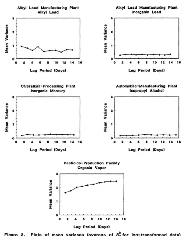
A breal<down by industry, however, quickly changes the interpretation of the data and

becomes extremely informative. Graphs for each of the five data sets are plotted in Figure 2. Of the

five data sets, only the pesticide-production facility shows a trend between the mean variance and the

lag. The alkyl lead manufacturing plant (alkyl lead and inorganic lead), the chloralkali-processing plant,

and the automobile-manufacturing plant data display no increase in the mean variance with lag.

These four data sets are characterized by relatively stable variances as the lag increases, although the

variance fluctuates slightly in alkyl lead exposures at the lead manufacturing plant. In contrast, the

pesticide-production facility data exhibits a significant increasing trend between variance and lag. Air

concentrations are highly variable, with mean values for the variance among pairs of measurements

from approximately 1.6 at lag 1 to around 2.4 at lag 10. These results indicate that the trend observed

in the combined data sets (Figure 1) arose in fact from the contribution of the pesticide-production

Alkyl Lead Manufacturing Plant

Alkyl Lead

2 4 6 8 10 12 14 Ifi

Lag Period (Days)

Alkyl Lead Manufacturing Plant

Inorganic Lead

2 4 6 8 10 12 14 16

Lag Period (Days)

o c

.3

*c

a

>

c

(0 «

2

2

Chloralkall-Processing Plant Inorganic Mercury

2 4 e 8 10 12 14 16

Lag Period (Days)

Automobile-Manufacturing Plant Isopropyl Alcohol

0 2 4 6 8 10 12 14 16

Lag Period (Days)

Pesticide-Production Facility Organic Vapor

« o

c

« (S

>

c

a 0)

2

0 2 4 6 8 10 12 14 16

Lag Period (Days)

Figure 2. Plots of mean variance (average of Sy for log-transformed data)

In an effort to further isolate the effect, data for each worker was assessed separately. None of

the data from the lead-manufacturing plant showed a discernible pattern between variance and lag.

Two plots shown in Figure 3 provide an illustration of the lack of trend between variance and lag in the

data generated at this facility. Graph A depicts data from Worker 4 exposed to alkyl lead while Graph B

plots the inorganic lead data for Worker 3. Both of these plots appear erratic and are characterized by

mean variances that fluctuate randomly with lag.

. Alkyl Lead Manufacturing Plant

A Alkyl Lead

B

Alkyl Lead Manufacturing Plant

Inorganic Lead

Worker 4

0.80

0.40

o.oo

Worker 3

4)

() /

C * /

Id A /

k. A / \ / 1

a

> 0.40

/ \ / \ 1

c

\ \ /

o 1 \ J* \ -/ 1 4) • w"'''^ \ m'"'^^

S

\J

0 2 4 6 8 10 12 14 16

Lag Period (Days)

0 2 4 6 8 10 12 14 16

Lag Period (Days)

Figure 3. Plots for two workers at the alkyl lead manufacturing plant.

Mean variances (average of Sy for log-transformed data) in both plots

appear to fluctuate randomly with lag.

data for Worker 15 in Figure 4-B at the pesticide plant is characterized by extremely large and variable

exposures, ranging from about 1.6 to over 3, whereas the values for the other two workers (Figures 5-B

and 6-B) are considerably smaller and less variable (ranging from 0.08 to 0.5). Overall, these results

suggest that the trend observed from the combined data set originates in the strings of 18 workers

from the pesticide production facility.

Pesticide-Production Facility

Organic Vapor

B

Pesticide-Production Facility Organic Vapor

Worker 10 Worker 15

8 10 12 14 IS 8 10 12 14 16

Lag Period (Days) Lag Period (Days)

0.20

Chloralkali-Processing Plant

Inorganic Mercury B

Worker 1 1

0.15

10 12 14 16

« o

c

.2

a

>

0.80

0.40

0.20

Chloralkali-Processing Plant

Inorganic Mercury

Worker 2

10 12 14 16

Lag Period (Days) Lag Period (Days)

Figure 5. Plots for two workers at the chloralkaii-processing plant.

Graph A shows no relationship between variance and lag whereas

Graph B displays a trend of increasing variance with lag. Variances

were computed using log-transformed data.

. Automobile-Manufacturing Plant

f^ Isopropyl Alcohol

B

0.20

Worker 1

0.16

Automobile-Manufacturing Plant

Isopropyl Alcohol

Worker 3

0.10

8 10 12 14 IS 18 0 2 4 6 8 10 12 14 16

Since some workers were sampled over longer intervals and contributed multiple strings of

data, the final analysis was conducted by individual time series to decipher differences over time.

Forty-five of the time series showed an increase of variance with lag. The majority (42) were drawn

from the data collected at the pesticide-production facility with the remaining series split between two

workers at the chloralkali-processing plant and one worker at the automobile-production plant.

The contrast between the analyses conducted by worker and by time series focused primarily

upon the pesticide-production plant where the overall trend arose. Although 64% of the workers

displayed an increasing variance with lag, it was found that approximately 2/3 of the data for these

workers showed no such trends. Thus, it appears that relatively few time series per worker dominated

the analysis. Figure 7 provides an illustration by plotting five time series for Worker 13 from the

pesticide facility. Three of the time series, graphs A-C, show no consistent trend between variance and

lag. In contrast, graphs D and E are characterized by marked upward trends, particularly in graph D.

The plot for Worker 13 combining all of the time series, in graph F, also shows a trend of increasing

variance with lag.

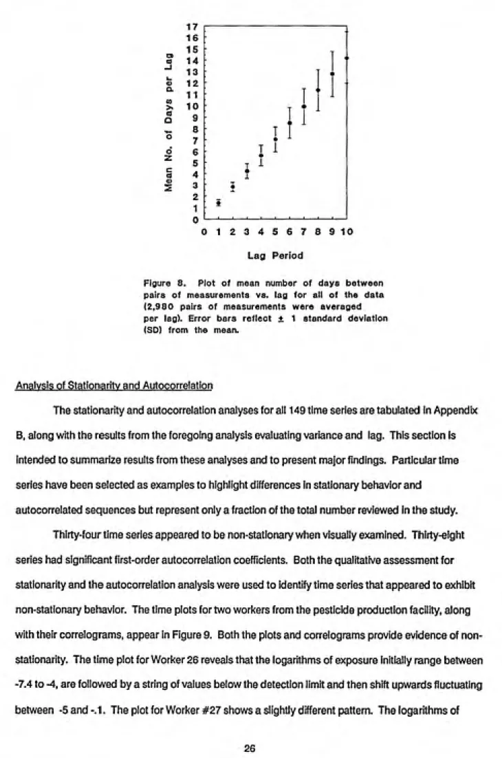
The unevenness in the spacing of the data due to absences and days of non-exposure was

assessed by averaging the number of days separating pairs of measurements for each lag period. The

data are tabulated for each analysis and appear in Appendix A. Figure 8 plots the relationship between

lag and the mean number of days for the analysis of the entire data base. For lags 1 and 10, the mean

was approximately 1.4 and 14.2 days, respectively (averaging values for 2,980 pairs of

measurements/per lag). Differences between the mean value and lag are relatively small suggesting

that missing data did not present significant problems. The comparisons were similar for the other

Seri«9 1 Series 2 Series 3

Worker 13 _{Worker 13} Worker 13

Lag Period (Days)

Series 4

Lag Period (Days) Series 5

Lag Period (Days)

Worker 13 Worker 13

0 2 4 6 S 1012141E1S20

Lag Period (Days)

0 2 4 6 S 10 12 14 1«

Lag Period (Days)

Combined Time Series

n

>

Worker 13

0 2 4 « 8 1012141618

Lag Period (Days)

Figure 7. Graphs A-D display five separate time series for Worker 13

at the pesticide plant. Graph F plots the combined data. Variances were

17 16 15 14 13 12 11 10 9 8 7 6 5 4 3 2 1 0

0123456789 10

Lag Period

Figure 8. Plot of mean number of days between

pairs of measurements vs. lag for all of the data

(2,980 pairs of measurements were averaged

per lag). Error bars reflect ± 1 standard deviation

(SD) from the mean.

Q. IB > CD O o z

: T

•

: T 1

•

•

• 1

1---0---1

•

Analysis of Stationaritv and Autocorrelation

The stationarity and autocorrelation analyses for all 149 time series are tabulated in Appendix

B, along with the results from the foregoing analysis evaluating variance and lag. This section is

intended to summarize results from these analyses and to present major findings. Particular time

series have been selected as examples to highlight differences in stationary behavior and

autocorrelated sequences but represent only a fraction of the total number reviewed in the study.

Thirty-four time series appeared to be non-stationary when visually examined. Thirty-eight

series had significant first-order autocorrelation coefficients. Both the qualitative assessment for

stationarity and the autocorrelation analysis were used to identify time series that appeared to exhibit

non-stationary behavior. The time plots for two workers from the pesticide production facility, along

with their correlograms, appear in Figure 9. Both the plots and correlograms provide evidence of

non-stationarity. The time plot for Worker 26 reveals that the logarithms of exposure initially range between

-7.4 to -4, are followed by a string of values below the detection limit and then shift upwards fluctuating

exposure remain relatively constant, drop to non-detectable levels and then rise to their highest values.

Note that the autocorrelation functions decay slowly to zero providing additional evidence of

non-stationarity. The correlograms need to be interpreted carefully, however, because of the string of

values in both plots below the detection limit.

Worker 26, Time Series 5

E

I

Worker 26, Time Series 5

ͣ

k o

Lag (k)

Worker 27, Time Series 2

m

ͣ

k 0

Worker 27, Time Series 2

Lag (k)

Figure 9. Time plots for two workers at the pesticide facility

appear on the left. The clashed lines on the correlograms represent

the approximate 9S% confidence limits. The autocorrelation functions

To contrast the trend in exposure seen in Figure 9, the time plot and correlogram for a worker

exposed to alky! lead at the lead-manufacturing plant are shown in Figure 10. The plot of air

concentrations over time shows no upward or downward movement suggesting a constant mean over

the period sampled. There also appears to be relatively little change in the variance. The

autocorrelation function behaves quite differently from the correlograms plotted in Figure 9, with none

of the autocorrelation coefficients significantly different from zero.

Worker 4, Time Series 1

0)

S

c

o

c <0 Q c o

O

Worker 4, Time Series 1

-1

-5 ^—

0 10 20 30 40 SO

012345678

Lag (k) Day

Figure 10. The time plot and correlogram for a worker exposed to

alkyl lead at the lead-manufacturing plant. Both graphs indicate

stationary behavior. Dashed lines on the correlogram represent

the approximate 9 5% confidence limits.

time plots. None of the longer strings from the pesticide-production facility, ranging between 61 and

140 measurements per string, were non-stationary by the formal test, although 36% (12 out of 33 plots)

were non-stationary by visual inspection.

Non-stationary series as assessed formally were transformed by differencing and re-tested. All

of the differenced series exhibited stationary behavior by the formal test; one time series was identified

as non-stationary by visual examination.

When the stationary series were examined for autocorrelation, 29 significant first-order

autocorrelation coefficients were detected. However, most of these (25) were barely significant. Only

four coefficients were larger than 0.5; all of these came from the pesticide-production facility. Figure

11 shows the time plot and correlogram for a series generating the highest coefficient (0.612). It can

be seen from the time plot that consecutive values are likely to be on the same side of the mean

(average value is -5.38). Twenty-six time series had significant coefficients at lags greater than one.

The physical significance of these coefficients is difficult to interpret and will not be considered further.

Worker 19, Time Series 1

y—5.38

Worker 19, Time Series 1

rk 0

012345678

Lag (k)

Figure 11. The time plot and correlogram for a worker exposed to

an organic vapor at the pesticide-production facility. The dashed

lines on the correlogram represent the approximate 95% confidence

Ten of the 14 non-stationary time series identified from the formal test showed no

autocorrelation after differencing. The differenced series producing significant results all had first-order

correlation coefficients that were negative and relatively large, contributing three out of the four highest

values. The significance of these coefficients requires careful interpretation. If a time series consists

purely of a trend and a stationary random component, then taking first differences will remove the

trend and result in a series whose sample autocorrelation function rapidly falls to zero (Gottman, 1981).

Figure 12 illustrates an example. The time plot for Worker 2 at the automobile-manufacturing plant

appears to linearly increase over time. The initial autocorrelation analysis yielded significant serial

coefficients for lags one through three (0.654, 0.485, 0.420, respectively) but this analysis is not valid if

the underlying process is non-stationary. The plot of first differences appears stationary (Figure 12-B);

the autocorrelation analysis on the differenced series produced no significant correlation coefficients.

6.00

Time Plot Worker 2, Series 1

5.50

5.00

4.50

S 4.00

3.50

Plot of First Differences

^ Worker 2, Series 1

E

O

c <u o c

o

o

10 20 30 40 50

Day Day

Figure 12. Time plot for a worker at the automobile plant shows a linear

increase over time. Taking first differences removes non-stationarity

In some instances, first differencing may not be an appropriate remedy for non-stationarity if

the series does not appear to increase linearly over time. To illustrate this point. Figure 13 shows the

time series for Worker 9 at the pesticide-production facility that was assessed as non-stationary by

both the formal test and visual inspection. Here no linear trend is evident (although there appears to

be some cycling) and the variance is not constant over time. Thus, the significant autocorrelation

coefficient obtained from the differenced data is suspect and may not be interpretable.

Time Plot

Worker 9, Series 7

E

c

«

u

+^

c 4> O c o

O

ft/1,

B

CD

E

c

o

c

O c o

O

Plot of First Differences

Worker 9, Series 7

lii /!/! /! li ! TM

10 20 30 40 50

Day

10 20 30 40 50

Day

Figure 13. Non-stationary time plot for a worker at the pesticide plant that

appears to cycle over time. Taking first differences may not be appropriate

as a means to remove non-stationarity.

To determine the extent to which autocorrelation or non-stationarity may explain the trend

between variance and lag among pairs of measurements separated by different intervals, the results

from these two analyses were coupled with the 45 time series displaying an increasing variance with

Dickey-including four negative coefficients obtained from the differenced series. Together non-stationarity and

autocorrelation explain the trend between variance and lag for 60% of the series.

Table 3. Results from the stationarity test and autocorrelation analysis for

time series where the variance increased along with the interval between

measurements.

Data Set Worker Time Test for

ist-Order 1

Series

Stationarity*

Autocorrelation |

Coefficient {

Pesticide-Manufacturing Plant

_{NS (NS)}

-0.537 +

7

_{NS (NS)}

-0.409+

6 3

NS (NS)

1

9 7

_{NS (NS)}

-0.510 +

8

_NS(S)

13 4

_NS(S)

₁

15 4

_{NS (NS)}

1

11

_{NS (NS)}

₁

24 1

_NS(S)

1

26 2

_{NS (NS)}

-0.571 +

5

_{NS (NS)}

-27 2

_{NS (NS)}

1

Automobile-Manufacturing Plant

_{NS (NS)}

1

*NS = Non-stationary; S = Stationary as assessed formally; values in parentheses are results

from visual inspection of the time plots.

+Autocorrelation performed on differenced series if assessed non-stationary by the formal

test; values in parentheses are results following differencing based on visual inspection of

Table 3 (Continued)

Data Set Worker Time Test for

Ist-Order 1

Series

_{Statlonarity*}

Autocorrelation |

Coefficient |

Pesticide-Manufacturing Plant

_S(NS)

_{0.397 (-0.474)+ 1}

7

_S(S)

11 3

_S(NS)

0.386 (-0.433) +

15 1

_S(S)

0.391 1

3

_S(S)

0.406 1

13

_S(S)

17 2

_S(NS)

_{0.495 (-0.676) +}

19 1

_S(NS)

_{0.612 (-0.612) +}

26 6

_S(NS)

0.367 (-0.451) +

27 1

₈₍₈₎

0.451 1

5

_S(NS)

0.424 (-)+ 1

28 2

_S(8)

4

_S(NS)

_{0.428 (-0.454) +}

Chloralkali-Manufacturing Plant

_S(S)

0.362 1

|Pesticide-Manufacturing Plant

_S(NS)

(-0.389) 1

6

_S(S)

1

6 5

_S(8)

1

6

_S(8)

1

7 7

_S(8)

_j

9

_S(S)

1

11 1

_S(NS)

_(-0.464)

4

_S(NS)

(-0.426) 1

12 2

₈₍₈₎

1

13 5

_S(S)

₁

14 1

₈₍₈₎

₁

15 5

_S(S)

1

10

_S(S)

1

21 1

_S(8)

₁

23 4

_S(8)

25 1

_S(8)

1

26 4

₈₍₈₎

₁

26 4

₈₍₃₎

1

Chloralkali-Manufacturing Plant

_S(S)

₁

*NS=Non-stationary; S=Stationary a

v; values in pare

CONCLUSIONS

Proper assessment of exposure requires that the variability in air concentration levels be taken

Into account. Specification of the variance Is generally considered In the context of a statistical

distribution of the underlying population of exposures. Such a distribution may be Incorrectly

specified, however, if day-to-day exposures are autocorrelated and this correlation is not statistically

assessed. Indeed significant errors in the estimated parameters can arise from campaigns of a few

days time (Francis etaj., 1989; Buringh and Lanting, 1991). Time-series analysis affords methods to

assess autocorrelation and to build a temporal component into the model describing exposures but

requires relatively long strings of consecutive measurements that are rarely collected In practice.

Given the lack of suitable data. Indirect methods may provide useful alternatives to traditional

time-series analysis (Buringh and Lanting, 1991). Specifically, a statistical property regarding the

variance has been used. Since positively autocorrelated data measured during brief Intervals will

underestimate the variability, differences between estimates of the variances between data collected

over brief intervals compared to longer time periods may provide some evidence of autocorrelation.

This analysis suggests that the validity of this indirect method depends upon careful control of

factors likely to contribute to variability, including industry, location, type of exposure, and worker. The

results confirm the observation of Buringh and Lanting (1991) that the variance tends to increase with

the interval between measurements. However, by controlling for the above confounding factors, this

analysis provided an additional opportunity to isolate the effect by data set, worker, and time series.

Isolation by data set showed that the trend was restricted to only one of the five data sets available for

investigation. Dissecting the data by worker and then by individual time series further revealed that the

trend was due to the influence of less than one-third of the time series.

The data set responsible for the observed trend was the largest both In terms of the number of

workers sampled and the number of time series contributing to the analysis. Besides dominating by

size, the data set was characterized by variances which were much larger than those of the other sets.

more general problem. It is possible that a data set with similar characteristics unduly influenced the

analysis conducted by Buringh and l_anting (1991).

Focusing now on the time series where the variance increased with lag, autocorrelation and

non-stationarity appear to have contributed to 60% of the trends. The significant first-order

autocorrelation coefficients range between 0.362 and 0.612. Some of these coefficients are small and

may have only contributed marginally to the observed trend. It is important to note, however, that over

half of the significant coefficients from the entire analysis were restricted to the series where the

variance increased with lag.

Finally, visual inspection of the plots for non-stationarity in the mean or variance appears to be

fairly robust when compared to the statistical test. The ad hoc method may in fact be preferable since

no underlying model is assumed and it is not constrained by small sample sizes, which can severely

limit the power of formal testing procedures. The percentage breakdown of the stationarity analysis for

the entire data set and for the various subsets of data appears in Figure 14.

VTVTVTVT

Entir* Series Longer Differenced

Data w/Trand Series Series

The issue of stationarity needs to be examined in greater detail. However, If our results are typical of

other workplaces, sampling strategies may not need to address problems associated with

REFERENCES

Buringh, E. and R. Lanting: Exposure Variability in the Workplace: Its Implications for the Assessment

of Compliance. >Am./nof.Hyfif.>Assoc. J. 52:6-13(1991).

Chatfield, C: The Analysis of Time Series: An Introduction. 4th ed. London: Chapman and Hall, 1989.

pp. 51-52.

Coenen, W.: Measurement Assessment of the Concentration of Health-Impairing, Especially

Silicogenic Dusts at Workplaces of Surface Industries. Staub Reinhalt. Luft 31:16-23 (1971).

Dickey, D.A. and W.A. Fuller: Distribution of the Estimators for Autoregressive Time Series with a Unit

Root. J. >Am.Sfaf. Assoc. 74:427-431 (1979).

Diggie, P.J. Time Series: A Biostatistical Introduction. New York: Oxford University Press, 1990. pp.

39-40, 45-46.

Esmen, N.: Retrospective Industrial Hygiene Surveys. Am. Ind. Hyg. Assoc. J. 40:58-65 (1979).

Francis, M., S. Selvin, R. Spear, and S. Rappaport: The Effect of Autocorrelation on the Estimation of

Workers'Daily Exposures. Am./nd. Hyg. Assoc. J. 50:37-43 (1989).

Fuller, W.A.: Introduction to Statistical Time Series. New York: John Wiley & Sons, 1976. pp.373.

Granger, C.W.J, and P. Newbold: Forecasting Economic Time Series. 2nd ed. Orlando: Academic

Press, Inc., 1986. pp. 4-5.

Gottman, J. M.: Time Series Analysis: A Comprehensive Introduction for Social Scientists New York:

Cambridge University Press, 1981. pp.95-96.

Kromhout, H., E. Symanski, and S.M. Rappaport: A Comprehensive Evaluation of Within- and

Between-Worker Components of Occupational Exposure to Chemical Agents. In preparation, 1992.

Preat, B.: Application of Geostatistical Methods for Estimation of the Dispersion Variance of

Occupational Exposures. Am./nd. Hygf. Assoc. J. 48:877-884 (1987).

Rappaport, S.M.: Assessment of Long-Term Exposures to Toxic Substances in Air. Ann. Occup. Hyg.

35(1):61-121 (1991).

Rappaport, S.M., H. Kromhout, and E. Symanski: Variation of Exposure Between Workers in

Homogeneous Exposure Groups. Am. Ind. Hyg. Assoc. J., submitted, 1992.

Rappaport, S.M. and R.C. Spear: Physiological Damping of Exposure Variability during Brief Periods.

Ana Occup. Hyg. 32:21-33 (1988).

Roach, S.A.: A Most Rational Basis for Air Sampling Programmes. Ann. Occup. Hyg. 20:65-84(1977).

Said, S.E. and D. A. Dickey: Testing for Unit Roots in Autoregressive-IVIoving Average Models of

Unknown Order. Biometrika 71:599-607(1984).

SAS, SAS Institute, Gary, NC, 1992.

Spear, R.C., S. Selvin, and M. Francis: The Influence of Averaging Time on the Distribution of

Exposures. Am./nd. Hyg. Assoc. J. 47:365-368 (1986).

APPENDIX A

Appendix A

IBREAKDOWN FOR ALL OF THE DATA

NObs Variable Minimum Maximum Mean Std Dev

149 MEAND1 0.8 2.35 1.387584 0.252816

149 MEAND2 1.8 4.4 2.786242 0.422943 149 MEAND3 2.5 5.9 4.215436 0.655458

149 MEAND4 3.3 8.45 5.613758 0.915332

149 MEAND5 4.2 9.95 7.043624 1.083776

149 MEAND6 4.85 11.8 8.477517 1.333982 149 MEAND7 5.75 14.15 9.891275 1.548678

149 MEAND8 6.55 16.35 11.31745 1.780676

149 MEAND9 7.35 18.45 12.74564 2.013442

149 MEAND10 8.15 21.1 14.18356 2.268173

BREAKDOWN BY DATA SET

Alkyl Leat

Manufacturing Plant (Alkyl Lead)

NObs Variable Minimum Maximum Mean Std Dev

4 MEAND1 1.15 1.55 1.375 0.184842

4 MEAND2 2.5 2.9 2.7875 0.193111

4 MEAND3 3.8 4.4 4.1 0.258199

4 MEAND4 5.1 5.8 5.4625 0.303795

4 MEAND5 6.7 7.25 6.9625 0.256174

4 MEAND6 8 88 8.4625 0.363719

4 MEAND7 9.2 10.3 9.85 0.479583

4MEAND8 10.5 11.7 11.25 0.544671

4 MEAND9 11.8 13 1 12.625 0.618466

4 MEAND10 13.2 146 14.075 0.670199

Alkyl Lead

Manufacturing Plant (Inorganic Lead)

NObs Variable Minimum Maximum Mean Std Dev

4MEAND1 1 3 16 1.3875 0.143614

4MEAND2 2.5 29 2.65 0.173205

4 MEAND3 39 4.45 4.1625 0.256174

4 MEAND4 51 57 5.375 0.25

4 MEAND5 65 72 6.875 0.377492

4MEAND6 8 86 8.275 0.320156

4 MEAND7 93 102 9.6875 0.458939

4MEAND8 106 118 11.1625 0.652399

4 MEAND9 118 132 12.525 0.780491

Appendix A

1 Pesticide-Manufacturing Plant

NObs Variable Minimum Maximum Mean Std Dev

120 MEAND1 0.8 2.35 1.382083 0.274382 120 MEAND2 1.8 4.4 2.779167 0.455433 120 MEAND3 2.5 5.9 4.1975 0.715872 120 MEAND4 3.3 8.45 5.593333 1.000881

120 MEAND5 4.2 9.95 7.003333 1.185694 120 MEAND6 4.85 11.8 8.428333 1.452262 120 MEAND7 5.75 14.15 9.834167 1.683184 120 MEAND8 6.55 16.35 11.25792 1.942374

120 MEANDg 7.35 18.45 12.67875 2.198574

120 MEAND10 8.15 21.1 14.10833 2.484011

|Chloralka

i-Processing Plant

NObs Variable Minimum Maximum Mean Std Dev

15 MEAND1 1.2 1.65 1.413333 0.140746

15 MEAND2 2.5 3.45 2.803333 0.268239

15 MEAND3 4 5.25 4.31 0.319151

15 MEAND4 5.4 6.8 5.71 0.414987

15 MEAND5 7 8.55 7.223333 0.466701

15 MEAND6 8.2 10.75 8.663333 0.742454

15 MEAND7 9.6 12.45 10.11 0.871616

15 MEAND8 11 13.7 11.51333 0.89092

15 MEAND9 12.5 15.4 12.97 0.933082

15 MEAND10 14 16.8 14.44333 0.924057

|Automobi

e-Manufacturing Plant

NObs Variable Minimum Maximum Mean Std Dev

6 MEAND1 1.35 1.55 1.441667 0.073598

6 MEAND2 2.6 3.25 2.975 0.238223

6MEAND3 4.2 4.8 4.45 0.204939

6MEAND4 5.65 6.3 6.041667 0.247824

6MEAND5 7.25 8 7.566667 0.284019

6 MEAND6 8.8 9.45 9.141667 0.26347

6MEAND7 10.05 11.25 10.65 0.475395 6 MEAND8 11.55 13 12.16667 0.564506

6 MEAND9 13 14.55 13.75 0.634035

Appendix A

IDATA SET AND WORKER

Alltyi Lead Manufacturing Plant (Aiityl Lead)

Worlcer=1

NObs Variable Minimum Maximum Mean Std Dev

MEAND1 1.15 1.15 1.15

MEAND2 2.85 2.85 2.85

MEAND3 4 4 4

MEAND4 5.35 5.35 5.35

MEAND5 6.8 6.8 6.8

MEAND6 8.35 8.35 8.35

MEAND7 9.8 9.8 9.8

MEAND8 11.2 11.2 11.2

MEAND9 12.5 12.5 12.5

MEAND10 13.9 13.9 13.9

Worker=2

NObs Variable Minimum Maximum Mean Std Dev

MEAND1 1.5 1.5 1.5

MEAND2 2.9 2.9 2.9

MEAND3 4.4 4.4 4.4

MEAND4 5.6 5.6 5.6

MEAND5 7.1 7.1 7.1

MEAND6 8.8 8.8 8.8

MEAND7 10.1 10.1 10.1 ,

MEAND8 11.6 11.6 11.6

MEAND9 13.1 13.1 13.1

MEAND10 14.6 14.6 14.6

Worker=3

NObs Variable Minimum Maximum Mean Std Dev

MEAND1 1.3 1.3 1.3

MEAND2 2.5 2.5 2.5

MEAND3 3.8 3.8 3.8

MEAND4 5.1 5.1 5.1

MEAND5 6.7 6.7 6.7

MEAND6 8 8 8

MEAND7 9.2 9.2 9.2

MEAND8 10.5 10.5 10.5

Appendix A

1 1

Worker=4

NObs Variable Minimum Maximum Mean Std Dev

MEAND1 1.55 1.55 1.55

MEAND2 2.9 2.9 2.9

MEAND3 4.2 4.2 4.2

MEAND4 5.8 5.8 5.8

MEAND5 7.25 7.25 7.25

MEAND6 8.7 8.7 8.7

MEAND7 10.3 10.3 10.3

MEAND8 11.7 11.7 11.7

MEAND9 13.1 13.1 13.1

MEAND10 14.6 14.6 14.6

JAIkyl Lead Manufacturing Plant (Inorganic Lead)

Worker=l

NObs Variable Minimum Maximum Mean Std Dev

MEAND1 1.3 1.3 1.3

IVIEAND2 2.6 2.6 2.6

MEAND3 4 4 4

MEAND4 5.3 5.3 5.3

MEAND5 6.6 6.6 6.6

!VIEAND6 8 8 8

[VIEAND7 9.3 9.3 9.3

MEAND8 10.6 10.6 10.6

MEAND9 11.8 11.8 11.8

MEAND10 13.2 13.2 13.2

Worker=2

NObs

Variable

MEAND1 1.6 1.6 1.6

MEAND2 2.6 2.6 2.6

MEAND3

l\/IEAND4 5.4 5.4 5.4

MEAND5 7.2 7.2 7.2

MEAND6 8.5 8.5 8.5