1239.pdf

TABLE OF CONTENTS

CHAPTER! INTRODUCTION...1

Objective of Investigation...2

CHAPTER 2 BACKGROUND/LITERATURE REVIEW...4

Environmental Regulations...7

Treatment of Metal Containing Wastewaters...9

CHAPTER 3 THEORETICAL CONSIDERATION & MODEL DEVELOPMENT...21

Metal Hydroxide Solubility...27

Metal Sulfide Solubility...28

Single Metal Precipitation Modeling...31

Multi-Metal Precipitation Modeling...46

CHAPTER4 RESULTS AND DISCUSSION...51

Single Metal Sulfide Precipitation...51

Multi Metal Sulfide Precipitation...71

CHAPTER 5 SUMMARY AND CONCLUSIONS...75

LIST OF TABLES

2-1 Heavy Metals Found in Major Industries...5

2-2 Metals Concentrations in Industrial Wastewaters ...5

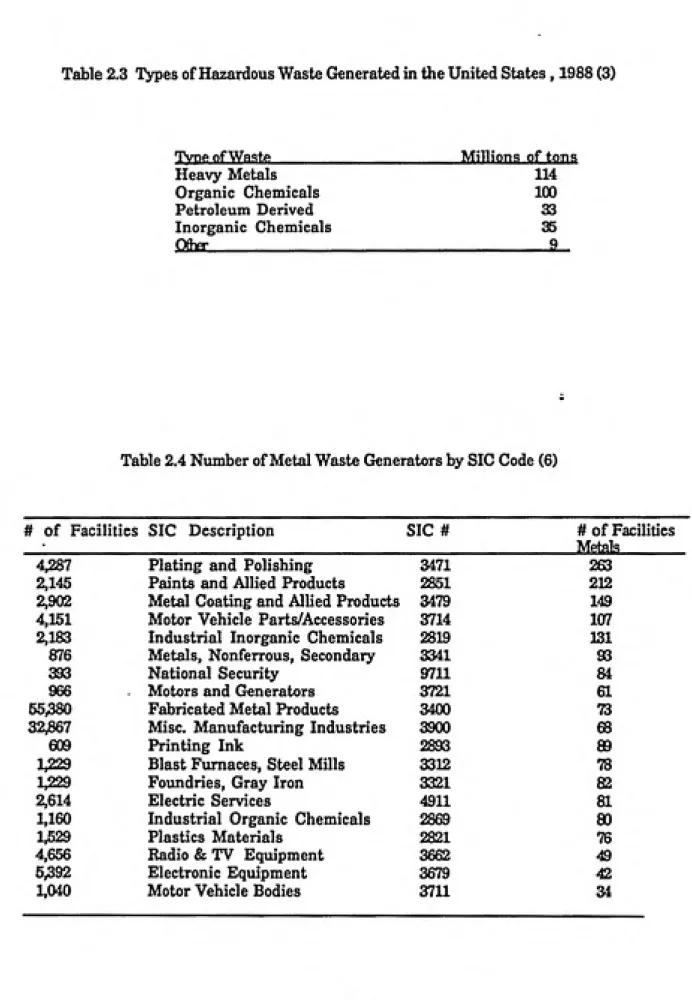
2-3 Types of Hazardous Waste Generated in the United States 1988...6

2-4 Number of Metal/Cyanide Waste Generators by SIC Code...6

2-5 Environmental Law and Regulations Affecting the Metals Industry...8

2-6 Pretreatment Standards for the Electroplating and Metal Finishing Industries...8

2-7 Theoretical Solubilities of Metal Hydroxide in Pure Water...ID 2-8 Hydroxide Precipitation Metal Removal Effectiveness ...10

2-9 Advantages and Disadvantages of Hydroxide Precipitation ...11

2-10 Advantages and Disadvantages of Sulfide Precipitation...35

2-11 Wastewater Treatment Process Detail of EPA Pilot Scale Tests...18

2-12 Chemical Analysis Wastewater Used in Pilot Tests...39

3-1 Stability Constants...23

3-2 Acidity Constants for Sulfide Species ...24

3-3 Comparison of Solubility Products of Metal Hydroxides and Sulfides ...26

3-3 Critical Sulfide Doses (Sent) With the Initial Metal Concentration = 3.5 x 10-5 M...35

3-4 Critical Sulfide Doses (Sent) With the Initial Metal Concentration = 3.5 x 10-3 M...35

3-5 Sulfide Dose Necessary to Achieve Only Sulfide Precipitation (S(-II)* With the Initial Metal Concentration 3.5 x 10-5 M...38

LIST OF FIGURES

2-1 Solubility of Metal Hydroxides as a Function of pH...13

2-2 Solubilities of Metal Hydroxides & Sulfides as a Function of pH...16

3-1 Calculated Distribution of Cadmium Species as a Function of pH...23

3-2 Calculated Distribution of Sulfide Species as a Function of pH...24

3-3 Calculated Solubilities of Various Metal Hydroxides...30

3-4 Calculated solubilities of Metal Sulfides as a Function of pH...30

3-5 Single Metal Precipitation Flow Chart...32

4-1 Residual Dissolved Fe(II) Concentration in the Absence of

Fe(0H)2(s) Precipitation pH 7 Initial Concentration 3.5 x lO^^ M...53

4-2 Residual Dissolved Fe(II) Concentration with the Coprecipitation of

Fe(0H)2 (s) at pH 10 Initial Fe(II) Concentration 3.5 x 10-3 m...53

4-3 Residual Dissolved Fe(II) Concentration in the Absence of Fe(0H)2 (s) Precipitation at pH7 Initial Fe(II) Concentration 3.5 x IQ-^ M...54

4-4 Residual Dissolved Fe(II) Concentration with the Coprecipitation of

Fe(0H)2 (s) at pH 10 Initial Fe(II) Concentration 3.5 x 10-5 m...54

4-5 Dissolved Sulfide Concentration and FeS(s) Precipitation in the Absence of Fe(0H)2 Coprecipitation at pH7 Initial Fe(II) Concentration 3.5 X 10-3 ^...58

4-6 Dissolved Sulfide Concentration and FeS(s) Precipitation in the Presence of Coprecipitating Fe(0H)2 at pHlO Initial Fe(II) Concentration 3.5 X 10-3 M...58

4-7 Dissolved Sulfide Concentration and FeS(s) Precipitation in the Absence of Fe(0H)2 Coprecipitation at pH7 Initial Fe{II) Concentration 3.5 X 10-5 M...99

List of figures (cont.)

4-10 Residual Dissolved Cd(II) Concentration with the Coprecipitation of Cd(0H)2 (s) at pH 10 Initial Cd(II) Concentration 3.5 x 10-3 M...62

4-11 Residual Dissolved Cd(II) Concentration in the Absence of Cd(0H)2 (s) Precipitation at pH 7 Initial Cd(II) Concentration 3.5 x 10-5 M...63 4-12 Residual Dissolved Cd(II) Concentration with the Coprecipitation of

Cd(OH)2(s) at pH 10 Initial Cd(II) Concentration 3.5 x 10-5 M...63

4-13 Dissolved Sulfide Concentration and CdS (s) Formation at pH 7

Initial Cd(II) Concentration 3.5x10-3 M...64

4-14 Dissolved Sulfide Concentration and CdS (s) Formation at pH 10

Initial Cd(II) Concentration 3.5x10-3 M...64

4-15 Dissolved Sulfide Concentration and CdS (s) Formation at pH 7

Initial Cd(II) Concentration 3.5x10-5 M...65

4-16 Dissolved Sulfide Concentration and CdS (s) Formation at pH 10

Initial Cd(II) Concentration 3.5x10-5 M...65

4-17 Iron Concentration, Sulfide Dose, and pH Conditions Necessary for Precipitation of Iron Sulfide...66 4-18 Nickel Concentration, Sulfide Dose, and pH Conditions Necessary

for Precipitation of Nickel Sulfide...67 4-19 Zinc Concentration, Sulfide Dose, and pH Conditions Necessary for

Precipitation of Zinc Sulfide...68 4-20 Cadmium Concentration, Sulfide Dose, and pH Conditions

Necessary for Precipitation of Cadmium Sulfide...69 4-21 Copper Concentration, Sulfide Dose, and pH Conditions Necessary

for Precipitation of Copper Sulfide...70 4-22 Selective Precipitation of CdS(s) In a Mixed Fe(II)-Cd(II) System at

pH 10 Initial Metal Concentration = 3.5 x 10-3 M...72 4-23 Dissolution of Fe(II and Cd(II) Hydroxide by Sulfide Addition at pH

10 Initial Metal Concentration = 3.5 x 10-3 M...72

Chapter 1

INTRODUCTION

Over the past two decades a growing awareness in the United States of the effects of industrial and municipal pollution has occurred. Many landfills, where much of the industrial waste has been deposited, have been identified as imminent health hazards due

to the leaching of inorganic contaminants to the soil and groundwater. (1) Typical heavy

metal contaminants include: iron, zinc, cadmium, copper, lead, mercury, and nickel. (2) Some of these metals are known to be toxic to humans, animals and plants. Heavy metals

pose a threat because they tend to accumulate in higher concentrations throughout the food

chain, multipljdng the hazard involved. Many metals play an essential role in the

function of living organisms. However, over-exposure to some of the heavy metals can

endanger human health or even cause death.

Numerous processes have been developed to remove metals from waste discharges. Traditional approaches utilized to treat metal-containing wastes include chemical precipitation, complexation, electrochemical operations, cementation, ion exchange, and membrane separation, to name a few. The primary method utilized in the United States for metal removal is chemical precipitation.(6) Through the addition of chemical reagents, metals can be precipitated as insoluble metal hydroxides, carbonates or sulfides.

The predominant chemical precipitation method for heavy metal removal is through

precipitation as an insoluble hydroxide at pH values between 8.5 and 11, The hydroxide

In more recent years, due to stricter wastewater effluent regulations, sulfide precipitation has been studied as an alternative to hydroxide precipitation for heavy metals removal. Theoretically, the sulfide process has a greater potential to comply with increasingly stringent effluent standards. The lower solubilities of metal sulfides allow for efficient precipitation even in mixed-metal wastes and in waste streams containing complexing agents. Other attractive features of the sulfide process include: precipitation of substantial amounts of soluble metal even at pH values of 2-3 (6), short detention times due to the high reactivity of sulfides, and the feasibility of selective metal recovery.

Objective of Investigation

The principal objective of this investigation was to assess the potential for using sulfide precipitation technology to remove heavy metals from mixed-metal containing wastewaters. A distinguishing feature of the sulfide precipitation process is the potential to selectively precipitate individual metals from mixed-metal containing waste streams.

In most precipitation processes, the treatment conditions lead to the concurrent precipitation of all metals in solution. Hence, the sludge produced is a mixture of all metals precipitated. Because some of the metals are regelated as hazardous materials under various federal statutes, any waste sludge containing concentrations of these metals above a threshold limit must be treated as hazardous waste. This categorization brings with it all of the regulations and requirements associated with hazardous waste treatment,

storage and disposal and significantly increases the cost and liability of managing the

the entire sludge is still considered hazardous. By optimizing sulfide concentration and pH , selective separation of certain metals can theoretically occur.

To this end, the specific objectives of this investigation include the following:

1. to develop the theoretical chemical equations necessary to describe conventional hydroxide and sulfide precipitation technologies;

2. to determine the theoretical effects of pH, sulfide dose, and metal concentration on

metal sulfide precipitation;

3. to assess the feasibility of employing sulfide precipitation technology as a pollution prevention strategy for metal-containing wastewaters.

The approach to this study is theoretical in nature. Prior to implementation of such a

full-scale sulfide precipitation process, laboratory and pilot-scale testing and verification

are recommended. A theoretical study is necessary, however, in order to assess the

potential for employing sulfide treatment technology, to establish the important operating

Chapter 2

BACKGROUND/LITERATURE REVIEW

The use of heavy metals in the United States is prevalent throughout many industrial

processes. Table 2-1 lists the broad range of industries utilizing heavy metals in their production processes. Typical concentrations of the heavy metals of concern from

industrial operations are shown in Table 2-2. As these two tables indicate, cadmium,

chromium, copper and zinc have widespread use across numerous industries.

Correspondingly, these metals have increasingly shown up as problems during waste treatment and disposal. A survey conducted in 1988 found that, overall, U.S. industries produced over 114 million tons of heavy metal wastes that were classified as hazardous wastes.(3) Table 2-3 lists the amount of hazardous metal wastes produced as compared to

the totals of other hazardous materials generated in 1988. Although this table shows that

metal-containing hazardous wastes were the largest portion of hazardous wastes generated

overall, it must be noted that not all sources of hazardous wastes are currently required to

report generation amounts.

The Environmental Protection Agency (EPA) requires various industries to report

the generation of hazardous materials, such as heavy metals, under several pieces of

environmental legislation. Table 2-4 identifies key industries that reported the

generation of metal wastes under the requirements of the Resource Conservation and

Recovery Act (RCRA) in the U.S. in 1983. Table 2-4 indicates that a majority of the metal

wastes are generated by the metal-processing, metal-finishing, and electroplating

industries(6). The exact composition of their waste streams is dependent upon the

Table 2.1 Heavy Metals Found in M^gor Industries (4)

Tnthrf^rv _{Al (V} rfl Or Ox T^ Tfr A&i Hi Tfi 7n

Pulp, paper mills,

papprboard, board mills X X X X X X

Organic chemicals

Petrochemicals X X X X X X X

Alkalis, Chlorine

Inorganic Chemicals X X X X X X J^

Fertilizers X X X X X X X X X _^

Petroleum refiningr X X X X X X X X

Basic steel works/foundrv X X X X X X X _?

X X X X X X X z

Auto/aircraft platinj X X X X X X X

Textile mill products

Lealiier tanning__________ _i_

Table 2.2 Metals Concentrations in Industrial Wastewaters (5)

Concentration (mg/1)

Metal Low 'Tvoical" High

Cadmium 1.0 25 5,000

Chromium (VI) 1.0 50 50,000

Copper LO 25 7,350

Iron 6.0 50 5,000

Lead 0.5 10 843

Mercury 0.005 1.0 1,920

Nickel 5.0 50 900

Table 2.3 Types of Hazardous Waste Generated in the United States , 1988 (3)

Type of Waste_______________________Millions of tons Heavy Metals 114 Organic Chemicals 100 Petroleum Derived 33 Inorganic Chemicals 36

Q&a:_________________________________________2_

Table 2.4 Number of Metal Waste Generators by SIC Code (6)

# of Facilities SIC Description SIC # # of Facilities

Metflls

4^7 Plating and Polishing 3471 263

2,145 Paints and Allied Products 2851 212

2,902 Met^ Coating and Allied Products 3479 149

4,151 Motor Vehicle Parts/Accessories 3714 107

2,183 Industrial Inorganic Chemicals 2819 131

876 _{Metals, Nonferrous, Secondary} 3341 S3

393 _{National Security} 9711 84

966 Motors and Generators 3721 61

55,380 Fabricated Metal Products 3400 73

32,867 Misc. Manufacturing Industries 3900 66

609 _{Printing Ink} 2893 89

1,229 Blast Furnaces, Steel Mills 3312 78

1,229 Foundries, Gray Iron 3321 82

2,614 Electric Services 4911 81

1,160 Industrial Organic Chemicals 2869 80

1,529 Plastics Materials 2821 76

4,656 Radio & TV Equipment 3662 49

5,392 Electronic Equipment 3679 42

Environmental Regulations

In addition to the hazardous waste reporting requirements, the U.S. EPA has

promulgated various environmental regulations which affect discharges of

metal-containing wastes from metal-finishing and metal-plating industry. The aim of this

environmental legislation is to reduce environmental exposure to toxic metals. These restrictions have increased the cost of disposing of wastes containing metal constituents, and in some cases prohibited the disposal of these wastes without prior pre-treatment. Table 2-5 lists the prominent environmental legislation affecting the metal-finishing

industry.

Some of the restrictions on the metal-finishing industries were enacted because

many metal-finishing and metal-plating companies discharge their wastewaters directly

to publicly owned treatment works (POTWs). The regulations often mandate

pretreatment of metal-containing wastes prior to discharge to POTWs because metals can inhibit aerobic and anaerobic biological treatment processes, thereby causing possible

deterioration of effluent quality and reduced rates of anaerobic sludge digestion.

Conventional municipal wastewater treatment plants are not typically designed to remove

heavy metals during treatment. As a result, even if the metals do not adversely affect the removal of BOD and suspended solids, many of the metals may pass through the plant and be discharged into the receiving waters. Metals present in treated sewage can be toxic to

aquatic life and can cause problems to downstream water users.(7) In addition, high

metal concentrations in municipal wastewater sludge can also limit the possibility of land

applications of the sludge, since metals can injure both crops and animals. The EPA pre¬

treatment standards for heavy metals from the electroplating and metal-finishing

Table 2.5 Environmental Law and Regulations Affecting the Metals Industries

Tjtw/Rtyiilation____________________DeSCriptJOn---40 CFR 122, NPDES Federal regulations governing the discharge of wastewaters

to surface waters of the U.S.

40 CFR 413,422 Federal regulations specifying effluent limitations, pretreatment standards, and new source performance standards for the electro¬

plating and metal finishing industries.

40 CFR 268 Federal regulations restricting the land disposal of untreated __________________________hazardous wastes_______________________________________

CFR = Code of Federal Regulations

NPDES = National Pollutant Discharge Elimination System

Table 2.6 Pretreatment Standards for the Electroplating and Metal-Finishing Industries(4)

Elfictronlating Rubcateyorv tEffluent Guidelines & Pretreatment Standards fmg/1)

Avg. Daily Value for

Metal_______________1-davMax__________________4 consecutive monitoring davs

2.7 2.6 4.0 2.6 0.4 0.7 6.8

Metal-Finishing Subcategorv : Effluent Guidelines & Pretreatment Standards Cmy/1)

Monthly average

Metal___________________1-day Max__________________shall not exceed

2.07 2.38 1.71 1.48 0.43 0.26 Copper 4.5 Nickel 4.1 Chrome.total 7.0 Zinc 4.2 Lead 0.6 Cadmium L2

Total metals 10.5

metals prior to discharge. Possible recovery of metals provides a ^ancial incentive to

study innovative treatment technologies to control metal discharges.

Typical processing procedures at metal-plating facilities include the dipping of

products into a series of plating baths containing various metals in order to achieve

desirable surface conditions. Contamination of these baths with oils, additional metals or

other contaminants occurs over time. When conditions of impurity exist, such that product

quality is impaired, it is necessary to replace these plating solutions. In addition to the

typical mixed-metal composition of these spent baths, the baths often contain high

concentrations of ammonia or cyanide. During the plating operation, the presence of

ammonia or cyanide allows for a desirable high concentration of soluble metals.

However, when treating the spent process waters, the presence of ammonia or cyanide

interferes with the precipitation of heavy metals.

Treatment of Metal Containing Wastewaters

Hvdroxide Precipitation

Hydroxide precipitation has been shown to efficiently remove heavy metals found in

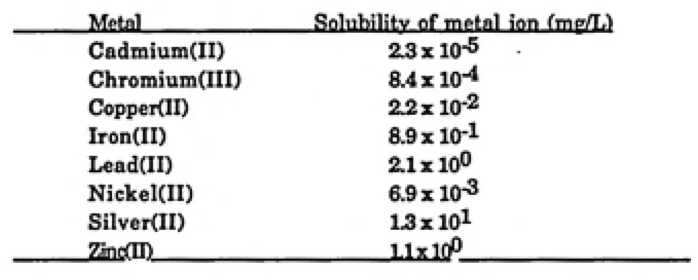
single metal-containing wastewaters (6). Table 2-7 lists the theoretical solubility of

various metal hydroxides in pure water (9). In comparison. Table 2-8 lists actual residual

concentrations which have been reported in the literature through the use of hydroxide

precipitation. (10) It is interesting to note that in the case of lead and zinc, the actual

residual concentrations shown in Table 2-8 are lower than the theoretical values reported

in Table 2-7. This suggests that the effectiveness of heavy metal hydroxide precipitation is

dependent not only on the hydroxide solubility product of the individual metal, but also on

Table 2-7 Theoretical Minimum Solubilities of Selected Metal Hydroxides in Pure

Water (9)

Cadmium(II) 2.3x10-5

Chromium(ni) 8.4x10-4

CoppeKII) 2.2x10-2

Iron(II) 8.9x10-1

Lead(II) 2.1xl00

Nickel(II) 6.9x10-3

Silver(II) 1.3x10^

ZincnD LlxloO

Table 2-8 Hydroxide Precipitation Metal Removal Effectiveness (10)

MM. Met Cone (mg/L) Residual Cpng (mg/L)

Cadmium(n) Chromium(ni)

Copper(n)

Iron(II) Lead(II) Nickel(II) ZJncfm________

ND

1.3xl03

2.0xl02-3.9xl02

1.0x10^

5.0x10-1-2.5x101

5.0xl00

-ISxlQl__________

7.0x10-4 6.0 xlO-2

2.0x10-1-2.3x101

1.0x10-1

3.0x10-2-1.1x10-1

1.5x10-1

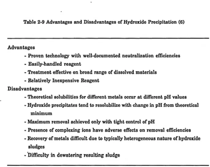
Table 2-9 Advantages and Disadvantages of Hydroxide Precipitation (6)

Advantages

- Proven technology with well-documented neutralization efficiencies

- Easily-handled reeigent

- Treatment effective on broad range of dissolved materials

- Relatively Inexpensive Reagent Disadvantages

- Theoretical solubilities for different metals occur at different pH values - Hydroxide precipitates tend to resolubilize with change in pH from theoretical

minimum

- Msiximum removal achieved only with tight control of pH

- Presence of complexing ions have adverse effects on removsil efficiencies - Recovery of metals difficult due to typically heterogeneous nature of hydroxide

sludges

While the hydroxide precipitation process has proven effective in single

contaminant waste streams, several problems have been noted with the use of hydroxide

treatment for heavy metal removal in more complex waste streams.(ll) Table

2-9 summarizes the advantages and disadvantages of employing a hydroxide treatment

process for heavy metals removal. Most metal hydroxides are amphoteric, that is the

hydroxide precipitate tends to resolubilize when the solution pH is altered from the

theoretical optimum due to the formation of soluble hydroxo-metal complexes. The

theoretical minimum solubility for most heavy metals occurs in the range of pH 9-11.

When the water is neutralized to a lower pH for discharge, some of the insoluble metal not

removed by sedimentation can redissolve. The precipitation of metals from a

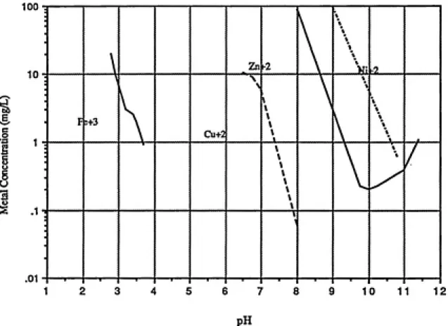
mixed-metal waste stream may not be effective using a hydroxide precipitation process because

the theoretical minimum solubility for each metal is narrow and may not overlap with that

of the other metals in solution. As seen in Figure 2-1, the ranges of minimum solubility for

different metals occurs at different pH values such that maximum removal can not be

achieved at the same pH for each metal. For mixed-metal wastes, it must be decided if one

pH value can remove all the harmful metals to an acceptable level.

In addition, hydroxide precipitation of metal-containing waste streams

contaminated by complexing agents may not be effective. Plating wastes contain

complexing or chelating agents used to brighten metals, clean equipment or keep metals

soluble. Ammonia, phosphates, and ethylenediaminetetraacetic acid (EDTA) are

luu ͣ: V \ ͣ _\ \ \ ͣ

V

\

ZnI2

\

V _{A \} \

1

\

\

^

ͣ

k

\

o ͣ Fs+3

\

\ \

\

\

1

i

\

/

^ .1 "! \\

<

«

.01 - —«---•

—'---\

---1---8 9 10 11 12

pH

Figure 2-1 Solubility of Metal Hydroxides as a Function of pH

Sulfide Precipitation

Precipitation of heavy metals by sulfide treatment technology occurs in a similar

manner to that of hydroxide precipitation.(14) In both cases, the soluble metal ions are

converted to insoluble metal compounds. Sulfide precipitation, however, has several

advantages over hydroxide precipitation. Table 2-11 lists several of the advantages of

employing a sulfide precipitation process (6). Primarily, the sulfide process was studied

because theoretically lower metal solubilities can be achieved through the use of sulfide

precipitation as can be seen in Figure 2-3 (15).

Typically, sulfide precipitation is conducted at pH values between 7 and 9.(15) The

amount of sulfide required to achieve substantial removal of metals is a fiinction of the

total metals concentration present in the metal-containing waste stream. For batch

treatment processes, jar tests can aid in determining optimal sulfide doses. In continuous

treatment processes, a sulfide specific electrode (16) can be employed to determine sulfide

demand. Numerous investigations have already proven the effectiveness of sulfide

precipitation of heavy metals fi-om industrial wastewaters. (15,17-25)

Two distinct processes exist for adding sulfide into metal-containing waste streams.

The difference between the two sulfide processes is the means of introducing the sulfide ion

into the wastewater. The soluble sulfide precipitation (SSP) process introduces the sulfide

as a water soluble sulfide reagent, such as sodium sulfide (Na2S) or sodium bisulfide

(NaHS). The insoluble sulfide precipitation (ISP)process provides sulfide ions through a

slightly soluble ferrous sulfide (FeS) slurry or calcium sulfide slurry (CaS). The iron

Table 2-10 Advanteiges and Disadvantages of Sulfide Precipitation

Advantages

- Ability to remove chromates and dichromates without separate pretreatment - High reactivity of sulfides with metals

- Insolubility of metal sulfides over broad pH range

- Relatively insensitive to the presence of most chelating agents Disadvantages

- Potential to produce hydrogen sulfide gas in acidic pH ranges - Excess sulfide necessary to drive reaction to completion

"•'f'm'wmffw^'

i

o

s

•s

> o

§

•a

i

PbOH)2

siem

Cu(OH)2

Cd(OH)2

—rbS

Figure 2-2 Solubilities of Metal Hydroxides and Metal Sulfides as a

with NaHS to produce a fresh FeS(s) slurry. The principle behind this process is that the FeS(s) will dissolve to a limited degree to produce both ferrous and sulfide ions according to the theoretical solubility product of FeS (s). As the sulfide ions are released from the solid iron slurry, they react with the heavy metals in the wastewater which have a solubility product less than that of ferrous sulfide. The Sulfex'"^*' method was developed to gradually introduce sulfide into the system to ensures that no colloid formation occurs due to the presence of excess sulfide. Colloid particles are difficult to remove and often require the use of membrane ultrafiltration to achieve adequate separation(13).

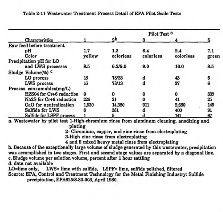
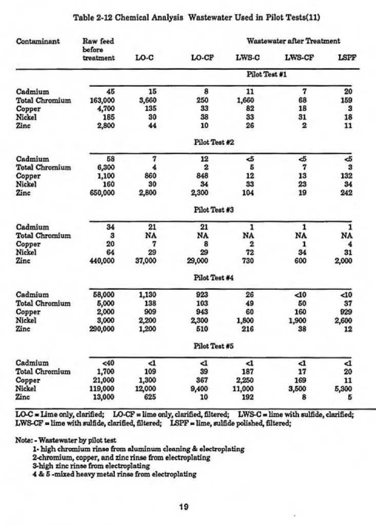
EPA discussed both of the sulfide precipitation techniques in a summary report (15) which indicated that addition of sulfide as soluble salts or as sparingly soluble metal sulfide slurry produces adequate metals removal. Several of their pilot studies compared and evaluated the SSP, ISP and hydroxide precipitation processes in systems open to the atmosphere. Five process variations were evaluated utilizing 14 actual raw wastewater samples. Results of the various pilot scale tests are presented in Tables 2-12 and 2-13.

Data fi-om the first pilot test shows that treatment with lime alone was adequate to

precipitate metals in the wastewater sample. By adding a filtration step, greater solids removal was achieved. In Pilot Tests 2 and 3, the wastewaters were not adequately treated by hydroxide precipitation alone. Improved effluent quality was obtained through addition of sulfide reagent. Mixed-metal wastes were tested in pilot runs 4 and 5. These runs indicate that low residual concentrations of all metals were not achieved by either hydroxide or sulfide precipitation treatment. Sulfide treatment did decrease the effluent concentrations of cadmium, copper and zinc; however, nickel concentrations remained

Table 2-11 Wastewater Treatment Process Detail of EPA Pilot Scale Tests

Pilot Testa

_______Characteristics___________ 1 2b 3 4 S

Raw feed before treatment

PH 1.7 1.2 6.4 2.4 7.1

Color yellow colorless colorless colorless _green

Precipitation pH for LO

and LWS processes 8.5 6.2/9.0 9.0 10.0 8.5

Sludge Volume(%) «

LO process 18 78/23 d 43 5

LWS process 16 78/13 d 37 6

Process consumables(mg/L)

H2S04 for Cr+6 reduction 0 0 0 0 339

Na2S for Cr+6 reduction 226 31 0 41 25

CaO for neutralization 1,530 14,380 9U 2,680 145

Sulfide for LWS 8 381 d 400 91

Sulfide for LRPF process 1 5 d 141 _ei

a. Wastewater by pilot test 1-High-chromium rinse from aluminum cleaning, anodizing and

plating

2- Chromium, copper, and zinc rinse from electroplating

3-High zinc rinse from electroplating

4 and 5 mixed heavy metal rinse from electroplating

b. Because of the exceptionally large volume of sludge generated by this wastewater, precipitation was accomplished in two stages. First and second stage values are separated by a diagonal line.

c. Sludge volume per solution volume, percent after 1 hour settling d. data not available

LO=lime only, LWS= lime with sulfide, LSPF= lime, sulfide polished, filtered

Source: EPA, Control and Treatment Technology for the Metal Finishing Industry: Sulfide

Table 2-12 Chemical Analysis Wastewater Used in Pilot Tests(ll)

Contaminant Raw feed Wastewater after Treatment

before

treatment LO-C LO-CF LWS-C LWS-CF LSPF

Pilot Test #1

Cadmium 45 15 8 11 7 20

Total Chromium 163,000 3,660 250 1,660 68 159

Copper 4,700 135 33 82 18 3

Nickel 185 30 38 33 31 18

Enc 2,800 44 10

Pilot Test #2

26 2 11

Cadmium 58 7 12 <5 <5 <S

Total Chromium 6,300 4 2 5 7 3

Copper 1,100 860 848 12 13 1^

Nickel 160 30 34 33 23 34

Zinc 650,000 2,800 2,300

Pilot Test #3

104 19 242

Cadmium 34 21 21 1 1 1

Total Chromium 3 NA NA NA NA NA

Copper 20 7 8 2 1 4

Nickel 64 29 29 72 34 31

Zinc 440,000 37,000 29,000

PaotTest#4

730 600 2,000

Cadmium 58,000 1,130 923 26 <10 <10

Total Chromium 5,000 138 103 49 50 37

Copper 2,000 909 943 60 160 929

Nickel 3,000 5?,200 2,300 1,800 1,900 2,600

Zinc 290,000 1,200 510

PaotTest#5

216 38 12

Cadmium <40 <1 <1 <1 <1 <1

Total Chromium 1,700 109 39 187 17 20

Copper 21,000 1,300 367 _2,250 169 11

Nickel 119,000 12,000 9,400 11,000 3,500 5,300

Zinc 13,000 625 10 192 8 5

LO-C = Lime only, clarified; LO-CF = lime only, clarified, filtered; LWS-C = lime with sulfide, clarified;

LWS-CF = lime with sulfide, clarified, filtered; LSPF = lime, sulfide polished, filtered;

Note: - Wastewater by pilot test

1- high chromium rinse firom aluminimi cleaning & electroplating 2-chromium, copper, and zinc rinse firom electroplating

3-high zinc rinse firom electroplating

Experimentsconducted by Hohman (26) evaluated the effects of oxygen on the dissolution of sulfide precipitates. In the presence of oxygen, sulfide can theoretically oxidize to sulfate, particularly at high temperatures and in alkaline solutions, thereby decreasing the extent of metals removal. The study reported that with no catalyst present, sulfide oxidation is limited for pH values below 6. Studies conducted at pH 8, the observed maximum oxidation rate, revealed that after 100 hours, 88% of the initial 100 mg/1 of sulfide was oxidized. The study also indicated that nearly 3 weeks were necessary to

oxidize the entire 100 mg/1 by atmospheric oxygen.

Hohman's studies of waste streams containing cadmium and iron showed that in systems open to the atmosphere, an immediate drop in the cadmium concentration occurred with sulfide addition. The iron concentration gradually declined. Preferential precipitation of cadmium over iron is expected for less than stoichiometic doses of sulfide. The amount of sulfide present was 33% of the stoichiometric dose for all metals present. The decrease in soluble iron concentration was attributed to oxidation of Fe(II) to Fe(III)

and subsequent precipitation of Fe(0H)3(s). In further studies, with 50% of the

stoichiometric addition of sulfide for all metals present, the final iron concentration was higher. The study attributed this to the oxygen demand exerted by the sulfide, which inhibited the oxidation of Fe(II) to Fe(III), and the formation of iron sulfide colloids which

did not precipitate.

Similar experiments were conducted under an imposed nitrogen environment to

minimize oxidation effects. Cadmium sulfide precipitation was efficient and rapid. The concentration of iron dropped initially and then subsequently rose throughout the remainder of the experiment. The final iron concentration was lower than in the open system. The overall experiments did show that adequate removal of both iron and

Chapters

THEORETICAL CONSIDERATIONS AND MODEL DEVELOPMENT

In order to predict the solubility of heavy metal systems, it is necessary to consider the distribution of metal hydrolysis products and, if sulfide is present, the distribution of protonated sulfide species. The following system of equations describes the hydrolysis

reactions for heavy metals in the +11 oxidation state.

Me2++ OH- = Me(OH)+ Ki (3-1)

Me2+ + 20H- = Me(0H)2 (aq) K2 (3-2)

Me2++30H- = Me(OH)3- Kg (3.3)

Me2+ +40H- = Me(OH)4 2- K^ (3-4)

With each of the above equations, an experimentally determined stability constant

(Kj) gives the relationship between the concentration of the products and the reactants. For

example, for Equation (3-1)

^ ^ [Me(0H)+1

^^ [ Me2+] [OH-] ^^^'

In general, for any of the hydrolysis products, the stability product, K{ relationship

can be written as follows:

^ rMe(OH)b ^(a-b)i

^ [ Me+a] [0H-] "

Similar equations can be written for the distribution of the sulfide species:

H2S(aq)= H++HS- Kal (3-8)

JHIHHSI

•^al "[HgSCaq)] ^^^'

HS- = H+ + S2- Ka2 (3-10)

[htyjS^

^«2 - [HS-] ' ^^-^^)

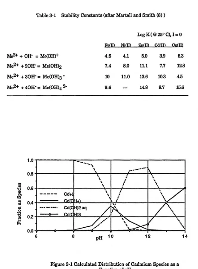
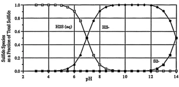
The stability constants for the hydrolysis products of iron(II), nickel(II), zinc(II), cadmium(II) and copper(II) are shown in Table 3-1. These stability constants can be used to produce a plot of the distribution of the aqueous species as a function of pH. Figure 3-1 is a graph of the distribution of soluble cadmium species as a function of pH using the stabiUty constants from Table 3-1. Table 3-2 presents the acidity constants for tiie sulfide species and Figure 3-2 shows the distribution of soluble sulfide species as a function of pH. The

distribution of sulfide species is important because of the toxicity of H2S (g). Below pH 5, neiu'ly all of the sulfide is present as aqueous H2S and the potential for H2S (g) evolution is

high in such systems.

In addition to the calculation of metal-sulfide hydrolysis products, one must consider the solubility product of both metal hydroxides and metal sulfides. For a heavy metal with

an oxidation state of +11, such as ferrous iron, nickel, zinc, cadmium and cupric copper,

Table 3-1 Stability Constants (after Martell and Smith (8))

LogK(@25''C),I = 0

Me2+ + OH- = Me(OH)+ Me2+ + 20H- = Me(0H)2

Me2+ + 30H- = Me(0H)3 "

Me2+ + 40H- = Me(0H)4

2-4.5 4.1 5.0 3.9 63

7.4 8.0 11.1 7.7 12.8

10 11.0 13.6 10.3 45

9.6 ... 14.8 8.7 15.6

i.u-n o _

\ _{*-••ͣ \ 1}

0.8 -\ \ \ • i •

\ 1

\ 1

\ 1 Q U.D

en

--- Cd+J

—... Cd(C

\ i

/

\ ^^ 1 \ ^/^ 1

m 0.4

-H)2 aq y

H)3 / ^

'V7---...

/\ 1

X *• 1

X \ 1 X \ 1

"ͣͣ'ͣ'ͣ"ͣ' GO(Q

o

no-1 "

ͣ

'.

0.0-1

,__v^^

/ \ 1

pH 10 12 14

Figure 3-1 Calculated Distribution of Cadmium Species as a

Table 3-2 Acidity Constants for Sulfide Species (after Martell and Smith (8))

H2S (aq) = H+ +

HS-HS- = H+ +

S2-@25°C.I=0

log Kai =-7.02

log Ka2 =-13.9

1.0

•I ^ 0.8 1

^ 0.6

So

11 0.4

•3 % 0.2

0.0

^.,

^

•1

H2S(aq)

\/

HS-N^

ͣ

1

Y

1

•1

/\

A

Mh-> ͣ I

S2- / 1

pH 10

12 14

Me(0H)2 (s) = Me2+ +2OH" (3-12)

The solubility product Kg^ for the dissolution of hydroxides is given by the following

expression:

Kso{OH) = [Me2+ ]I0H-]2 (3-13)

The same type of equation can be written for the solubility of metal sulfides:

MeS(S) =Me2+ + $2- (3-14)

Kso(S) =[Me2+ ][S2- ] (3-15)

The Kgo values for metals sulfides and metal hydroxides are compared in Table 3-3.

Table 3-3 Comparison of Solubility Products of Metal Hydroxides and Sulfides (8)

@h_=0,25°C

Metal Ions

LogKgoof

Metal Sulfide

LogKsoOf

Metal Hydroxide

Fe(II) -lai -15.10

Ni(II) -19.4 -15.20

Zn(n) -24.7 -15.52

CdCH) -27.0 -14.35

Metal Hydroxide Solubility

Metal hydroxide solubility is controlled by pH. To calculate the solubility for a

single metal hydroxide, Me g^j, the hydroxide solubility product from Equation (3-13) is

used along with the concentration of hydroxide ion (OH ") and a mass balance on the total Me gQi concentration, in the following manner:

'^'-TS^ (3-16)

[OH]=10(PH-14) (3.17)

Me sol= [Me2+] + [MeOH+] + [Me(0H)2 (aq)] + [Me(0H)3"] + [Me(0H)4 2-] (3-18)

Equation (3-18) can be rewritten in terms of the free metal ion concentration [Me^+l,

the hydroxide ion concentration [OH'] , and stability constants from Equations (3-1)

through (3-4).

Me sol= [Me2+] + Ki [Me2+] [OH"] + K2 [Me2+] [OH'] 2 + K3 [Me2+l [0H-]3+ K4 [Me2+] [OH" f

= [Me2+](1 + Ki [OH- ] + K2 [OH- ] 2 + K3[0H- ] 3 + K4 [OH- ] 4)

= [Me2+](fMe(0H)) (3-19)

From Equation (3-16) IMe2+ ]= !,^J°"^

and therefore Me sol = ^^^^^^2 (^Me(OH)) (3-19b)

Figure 3-3 presents the calculated dissolved metal concentration for several metals

as a function of pH using Equation 3-19b.

Metal Sulfide Solubilitv

The solubility of a metal sulfide can be calculated in a similar manner as that for

metal hydroxide solubility. A mass balance on total soluble sulfide species, Sgg}, is also

necessary.

S sol= [S2-] + [HS-] + [HgS (aq)] (3-20)

Returning to the acidity constants of Equations (3-9) and (3-10), Equation (3-20) can

be rewritten as follows:

^-'^^•"-e^Ki?^'

= [S2T(fs) (3-21)

where (^S) = 0+i?^+k^^^^J---)

ͣ

(3-21a)

The free metal concentration can now be calculated from equations (3-15) and (3-21).

The total soluble metal concentration Megoj, including the dissolved hydrolysis

species is then calculated through a combination of Equations (3-19) and (3-21).

Figure 3-4 presents the calculated dissolved metal concentration for several metals

as a function of pH with a 3.5 x 10*^ M sulfide addition. It can be seen in Figures 3-3 and

TOtKel

Calnuum

€< ipeer

8 pH 10

Figure 3-3 Calculated Solubilities of Various Metal Hydroxides

o

Ntekel

Caanrnint

Single Metal Precipitation Modeling Soluble Sulfide Addition

The equations established in the previous sections establish the maximum soluble concentrations of various metals in hydroxide systems or sulfide systems at specific pH values and specified dissolved sulfide concentrations. Real metal systems do not necessarily behave as separate functions. There are numerous variables which determine their potential precipitation behavior. In order to adequately model a real system, it is important to anticipate all the possible precipitation scenarios and prepare a model which could predict the entire system by including both hydroxide precipitation and sulfide precipitation. The initial conditions of the system, that is total metal concentration, pH, and total sulfide added, could be input to a program which would then calculate the predicted equilibrium concentrations of the soluble species, and from those values the

model could calculate the amount of metal precipitated as either a hydroxide or sulfide.

Figure 3-5 presents a fiow chart of the basic questions asked in the model.

For a single metal system with sulfide added, two results are generally possible:

1) Both Hydroxide and Sulfide precipitates are formed.

2) Only Sulfide precipitation occurs.

To begin to evaluate the system, the initial metal concentration Me^^g^, and pH

conditions would be input. The question that the model would attempt to answer is what

concentration of soluble sulfide, Sg^], is necessary to produce the desired residual metal

concentration, and therefore how much total sulfide, S>j<, needs to be added eii^er as a

Input Inital Conditions: pH

Initial Metal Concentration (Me tot)

Mesd = E(pi3-19b Me(OH)2(s) = MetcA - Me sd

M^al

No

Hff 1 -kA- 1 1

Mesol - ivjB lUL 1

^---Input Sulfide added (Stot)

Will Metal Precipitate

as a Metal Sulfide?

S crit determined by

Eqn. 3-26

SC-ID* = Me(OH)2 (s) - Ssol

Ssol = Eqn. 3-15, 3-19b, 3-13

Predpitaticai of Metal Sulfide

only Co-predpitaticKi of

Metal Sulfide and

Metal Hydroxide No sulfide

Precipitation

Report Metal spedes fixm earlier calculations

S sol = Stot

Me sd = Eqn 3-13 & 3-19b

Ssd = Eqn 3-13 & 3-26 MeS (s) = Eqn 3-27 Me(OH)2(s)= Eqn 3-28

Me sd = Eqn 3-19b & 3-37

S sol = Ecjn 3-13 & 3-26

and solubility products associated with the individual metals, the soluble metal concentrations at the specified pH value can be calculated from Equations 3-16 and 3-19b.

Sulfide Precipitation Concurrent With Hydroxide Precipitation

If sulfide is present in the system, it is necessary to determine if sulfide precipitation will occur concurrently with the hydroxide. If both Me(0H)2 (s) and MeS (s) co-precipitate,

the conditions of Equations 3-13 and 3-15 must be met simultaneously.

^^^ ^ [ OH- ]2-[S 2- ] ^=^25)

The pH value establishes the concentration of free Me ^"^j and thus the concentration

of total soluble metal, Megoj from Equation 3-20b. The concentration of free S ^' is also

fixed from Equation 3-15 . With the free sulfide concentration known, the amoimt of total soluble sulfide that can co-exist with both solid phases can be easily calculated from

Equations 3-21 and 3-25.

Scrit=-ir^-^([OH"l^)(^S) (3-26)

Therefore, at this total sulfide dose equal to S g^], the concentration of free Me *^ must

be in equihbrium with both solid phases and Equation (3-25) must hold. By establishing a

balance on total sulfide in the system, the amount of insoluble metal that precipitates as

sulfide can be calculated:

MeS (s)=S(-II) added -S sol 0-27)

Finally, the amount of insoluble metal that precipitates as a hydroxide can be

Me (0H)2 (s) = Me ^t - Me gQi - MeS (s) (3-28)

Tables 3-3 and 3-4 give the critical concentrations of sulfide, S^.^^, necessary to

initiate precipitation as a sulfide for iron(II), nickel(II), zinc(II), cadmium(II) and

copper(II) at pH values from 3 to 14 for initial metal concentrations of 3.5 x 10"^ M and 3.5

X 10"3 M, respectively. If S(-II) added> S^'^I^crit' *^®" precipitation as a sulfide will occur

concurrent with hydroxide precipitation according to Equations 3-25 through 3-28.

Because the free metal is fixed by the hydroxide term in Equation 3-25, the soluble metal concentration remains constant during the region of co-precipitation of both the metal sulfide and the metal hydroxide. In addition, the soluble sulfide concentration is also constant over this same range (see Equation 3-26). As the added sulfide dose is increased from the critical dose, more metal sulfide precipitates and the amount of hydroxide precipitating decreases proportionally with the increasing amount of sulfide precipitating as indicated by Equation 3-28. The above relationship holds until there is no longer any metal hydroxide precipitating from the system. This sulfide dose, S(-II) , at which only a sulfide precipitate is present is of importance in a selective precipitation model. Sulfide additions greater than S(-II) will create favorable conditions for single

metal sulfide precipitation.

The S(-II) dose can be easily calculated if the initial concentration of metal. Me ^^^

is known. As sulfide is added to the system, it speciates as H2S, HS" and S'^ depending

Table 3-3 Critical Sulfide Doses (Sgrit) M Initial Metal Concentration = 3.5 x 10'^ M

1 ^

3^ 1.89E+01 9.46E-01 4.74E-06 2.38E-08 1.89E-17 4^ 1.89E-01 9.47E-03 4.75E-08 2.38E-10 1.89E-19

5JO0 1.91E-03 9.55E-05 4.79E.10 2.40E-12 1.91E-21

&00 2.07E-05 1.04E-06 5.20E-12 2.60E-14 2.11E-23 7^ 3.70E-07 1.85E-08 9.37E-14 4.65E-16 2.70E-24 &00 2.05E-08 l.OlE-09 6.13E-15 2.53E-17 1.46E-23 9^ 8.03E-09 5.06E-10 6.69E-15 2.49E-18 1.33E-22 10.00 7.95E-08 5.02E-09 5.94E-14 1.78E-17 1.32E-21 11.00 7.95E-07 5.02E-08 7.55E-13 1.78E-16 1.32E-20 12.00 8.04E-06 5.08E-07 2.69E-11 1.80E-15 1.33E-19 13.00 8.94E-05 5.64E-06 5.31E-09 2.00E-14 1.48E-18 14.00 1.79E-03 2.04E-04 6.86E-06 1.06E-12

1.75E-161

Table 3-4 Critical Sulfide Doses (Scrit) M

Initial Metal Concentration = 3.5 x 10'3 M

1 ^

3J00 1.89E-01 9.46E-03 4.74E-08 2.38E-10 1.89E-19 4.00 1.89E-03 9.47E-05 4.75E-10 2.38E-12 1.89E-21 5Mi 1.91E-05 9.55E-07 4.79E-12 2.40E-14 1.91E-23 &00 2.07E-07 1.04E-08 5.20E-14 2.60E-16 1.51E-24 IJOO 3.70E-09 1.85E-10 9.37E-16 4.65E-18 2.70E-24 &00 8.78E-10 5.54E-11 5.80E-16 2.53E-19 1.46E-23 9.00 8.03E-09 5.06E-10 5.30E-15 1.80E-18 1.33E-22 10.00 7.95E-08 5.02E-09 5.25E-14 1.78E-17 1.32E-21 11.00 7.95E-07 5.02E-08 5.26E-13 1.78E-16 1.32E-20 12.00 8.04E-06 5.08E-07 5.31E-12 1.80E-15 1.33E-19 13.00 8.94E-05 5.64E-06 5.91E-11 2.00E-14 1.48E-18

hydroxide precipitate has been dissolved that a decrease in the soluble metal concentration

is observed.

At the point when there is no hydroxide precipitate left in the system, the total metal in the system is equal to the amount of soluble metal present plus the amount of metal which precipitates as metal sulfide. In addition, the total sulfide present in the system is equal to the amount of soluble sulfide plus the amount of sulfide which precipitates as metal sulfide.

Metot = Mesoi + MeS(s) (3-29a)

Stot = Ssol + MeS(s) (3-29b)

These two equations can be combined to determine the total amount of sulfide

necessary to achieve only sulfide precipitation.

Slot ͣSsol=^''e tot - Mfisol (3-29C)

where

_{Mesoi = IMe2+](f^^e(OH))}

and _{Ssol=[S2-l(fs)} from Equation 3-21

The free metal concentration at the point when all the hydroxide precipitate has been

dissolved is controlled by the metal hydroxide solubility product. (Note: Beyond this point,

the free metal concentration would be controlled by the metal sulfide solubility product)

By combining the Equations 3-16,3-19,3-21 and 3-29c an equation solving for the total

sulfide needed, S(-II) , can be determined.

S(-IIHMetot-Y^^j^TV(*Me(OH))^^^^^ (3-30)

\*

Tables 3-5 and 3-6 present S(-II) doses for pH values 3 to 14 for iron(II), nickel(II),

zinc(II), cadmium(II) and copper(II) with initial metal concentrations of 3.5 x 10 "^ M and

3.5 X 10 '3 M respectively. It should be noted from these two tables that at lower pH values

when no metal hydroxide forms initially, the S(-II) dose is equal to the Sgrit dose, the

sulfide dose necessary to achieve only sulfide precipitation with no metal hydroxide

coprecipitating.

Sulfide Precipitation Without Hydroxide Precipitation

For the case where only a sulfide precipitate is formed, the following equations are

utilized to calculate the free metal concentration:

Me tot= MSsol + ^®S (S) (3-31)

Stot=Ssol + MeS(s) (3-32)

Kso(S) =[Me+2 ][S-2 ] (3-15)

This system of equations can be manipulated and solved for [ Me *^ ]. By subtracting

Equation 3-32 from Equation 3-31, the MeS (s) term can be removed producing:

^®tot _ͣ Stot=^®sol" ^sol (3-33)

Megoi and Sgol can be replaced with Equations containing [ Me *^ ] and [ S "^ ]

Table 3-5 Sulfide Dose Necessary to Achieve Only Sulfide Precipitation (S(-II) )

No Me(0H)2 (s) Coprecipitation; Initial Metal Concentration 3.5 x 10"^ M

1 ^

3J00 1.89E+01 9.46E-01 4.74E-06 2.38E-08 1.89E-17

4J00 1.89E-01 9.47E-03 4.75E-08 2.38E-10 1.89E-19

5J00 1.91E-03 9.55E-05 4.79E-10 2.40E-12 1.91E-21

ejoo 2.07E-05 1.04E-06 5.20E-12 2.60E-14 2.11E-23

7.00 3.70E-07 1.85E-08 9.37E-14 4.65E-16 2.90E-05 &00 2.05E-08 l.OlE-09 6.13E-15 2.53E-17 3.46E-05

9.00 2.45E-05 2.78E-05 6.69E-15 2.49E-18 3.47E-05

10.00 3.47E-05 3.48E-05 5.94E-14 3.40E-05 3.47E-05

11.00 3.57E-05 3.49E-05 7.55E-13 3.46E-05 3.47E-05

12.00 4.29E-05 3.48E-05 2.69E-11 3.39E-05 3.45E-05

13.00 1.24E-04 3.43E-05 5.31E-09 2.58E-05 3.13E-05

1 14.00

1.75E-161

Table 3-6 Sulfide Dose Necessary to Achieve Only Sulfide Precipitation (S(-II) )

No Me(0H)2 (s) Coprecipitation; Initial Metal Concentration = 3.5 x lO"^ M

1 ^

3J00 1.89E-01 9.46E-03 4.74E-08 2.38E-10 1.89E-19

4.00 1.89E-03 9.47E-05 4.75E-10 2.38E-12 1.89E-21 5.00 1.91E-05 9.55E-07 4.79E-12 2.40E-14 1.91E-23

e.00 2.07E-07 1.04E-08 5.20E-14 2.60E-16 3.01E-03

7.00 3.70E-09 1.85E-10 9.37E-16 4.65E-18 3.49E-03

8.00 2.68E-03 2.86E-03 3.13E-03 2.53E-19 3.50E-03

9.00 3.49E-03 3.49E-03 3.46E-03 3.46E-03 3.50E-03 10.00 3.50E-03 3.50E-03 3.46E-03 3.50E-03 3.50E-03 11.00 3.50E-03 3.50E-03 3.45E-03 3.50E-03 3.50E-03

12.00 3.51E-03 3.50E-03 3.32E-03 3.50E-03 3.50E-03

13.00 3.59E-03 3.50E-03 3.54E-04 3.49E-03 3.50E-03

Me tot - S tot= IMe+2] (f ^e) - lS-2] (f s) (3-34)

By inserting Equation 3-15 into Equation 3-34 the [S"^] term is removed leaving:

-lMe+2](fMe) + (Metot-Stot) + j^;^2?Y" ^*^'° ^^'^^^

Multipljdng through by [Me"'"^] produces the following quadratic equation of the form

-b±Vb2-4ac ax^ + bx + c = 0 with x equal to ͣ _2a

- lMe+2]2 (f ^q) + (Me tot - S tot) [Me+2] + Kgo (S) (t s) = 0 (3-36)

with x=[Me+2]

a=-1(1+Ki[OH] + K2[OH]2 + K3[OH]3+ K4lOH]4)= - (i ^^)

b=Metot - Stot

<^Kso(S)(1-]?^-Hi^) =Kso(S)(fs) .

„r ma^^^ ' ^"^^tof ^<ot^' ^^^^ tot • S tot)^ +4 (- fMe) (Kso IS)) (^S) ,^^^

or [Me J - 2{-fMe)

Once the free metal concentration is calculated from Equation 3-37 for a known dose of total sulfide, a given amount of total metal and a given pH, the amount of soluble metal and MeS (s) precipitated can be calculated from Equations 3-19 and 3-31 respectively.

Insoluble Sulfide Addition usiny Ferrous Sulfide

ions, it is necessary to determine if iron will precipitate as iron hydroxide at the treatment

pH.

Fe (ID Controlled hv FefOH^^

If Pe(0H)2 precipitates, the [Pe^'*'] concentration will be fixed by the following

jPg2+] =^^alMdi. (3.38)

[OH-]

Once the free metal concentration is known, the sulfide ion concentration is calculated from the solubility product of iron sulfide Equation 3-15 and Equation 3-38.

•^SO (FeOH)

In a system of mixed metals, the additional metal concentrations must be in equiUbrium with the fi"ee sulfide as well. For example, if the solution contains cadmium, the fi'ee cadmium in equilibrium with the sulfide ions released from the iron sulfide

slurry is calculated as follows:

lCd2-Hl=^^^l^ (3-40)

or [Cd2+]=-—---^smedS)--- (3.41)

Kso (FeOH)

equilibrium is reached in accordance with Equation 3-41. The soluble cadmium concentration can be calculated from Equation 3-41 and Equation 3-19. As the free sulfide is consumed by the cadmium in forming cadmium sulfide precipitate, additional ferrous sulfide will dissolve. As long as the iron sulfide slurry is present in excess, the cadmium will precipitate as cadmium sulfide and no cadmium hydroxide will be formed due to the fact that cadmium sulfide has a lower Kgo value than cadmium hydroxide. The amount of cadmium sulfide that will precipitate can be calculated from a mass balance on cadmium.

CdS(s) = Cd,otai-Cdsoi (3-42)

The model should predict the amount of iron sulfide slurry necessary to provide enough sulfide ions to precipitate the metal of concern. A mass balance on sulfide species will determine the amount of sulfide that dissolved fi'om the added iron sulfide slurry.

S(-ll)diss = S(-ll)sol + CclS(s) (3-43)

By combining Equation 3-43 with Equations 3-19, 3-21,3-41, and 3-42 the amount of sulfide

released is given by the following equation:

S(-ll) diss= tS2-] (f S) + Cdtotal - (-—irrt^^--- (f CdOH)) (3-44)

J^gQ ^^^^^ I0H-]2

Kso (FeOH)

The amount of sulfide released is equal to the amount of total iron released provided

that no iron was initially present in the wastewater. From this mass balance on FeS (s) dissolved, it is possible to determine how much iron precipitates as iron hydroxide and how much iron sulfide was dissolved. (Note:The model assumes that no oxidation of sulfide or

Fedjssolved = S(-ll)dissolved (^-45)

Fedissolved = Fe(ll)sol + Fe(OH)2(s) (3-46)

By manipulating the equations developed earlier, the Fe(0H)2 (s) can be calculated

as follows:

Fe(0H)2(s) = Fedissolved - Fesoi (3-47)

Combining Equation 3-44, 3-45, and 3-47, the following relationship can be developed.

Fe(0H)2 (s) = ([S2-] (f s) + Cdtotai - (-]<---T^^^T^---— (^ CdOH)) -Fegoi (3^)

•^SO (FeOH)

The [S^"] can be replaced with Equation 3-39 and Fcgoi can be replaced with Equation

3-19b to develop a relationship in which all unknowns are a function of pH.

Fe(0H)2(s) = K^f l^'^;^) [0H-]2 (fs)+ Cdtotai - i—iCTTf^---(^CdOH))

_{^SO (FeOH) ___^SO (FeS) [0\^-] 2}

Kso (FeOH)

-%Sf^(*FeOH) (3-49)

which indicates that the amount of iron sulfide that dissolves is a function of pH and of the

quantity of less soluble metals, e.g. Cd (II), that are present. As a final step, the amount of iron sulfide dissolved can be calculated from a mass balance on the iron species.

TJ ||;;;l|| '_ i r H.f !,^, jljl J .jlfj^'l'j

-And finally, the amount of iron suMde remaining can be calculated by simple

subtraction:

FeS(s) added- FeS(s) c»nsumed = FeS(s) remaining (3-51)

Therefore, the presence of iron hydroxide precipitate fixes the concentration of free sulfide and consequently establishes the maximum soluble cadmium concentration from

Equations 3-38 through 3-41:

Cd sol - ^'^ ^^^^^ '''Vo^-?2 (^ CdOH)) (3-51a)

Equation 3-5 la indicates that the residual cadmium concentration is independent of the amount of iron sulfide slurry added. This equation only applies when the iron sulfide slurry is present in excess. In the cases when no FeS(s) remains, the free iron concentration is not fixed by Equation 3-13, but rather Fesol is equal to the amount of iron sulfide added to the system due simply to the dissolution equilibrium shown below:

Fesol = FeS(s) added (3-51 b)

The free iron is determined from Equation 3-19. The soluble cadmium concentration is also dependant upon the amount of iron sulfide slurry added. The soluble sulfide is equal to the amount of FeS(s) added, again simply due to the dissolution of the iron sulfide slurry.

Ssol = FeS(s) added (3-51c)

^ «>' = %'!^?.?lJL (* CdOH)) (3-51d)

No Precipitation of FefOH^o fs^

If a hydroxide precipitate is not formed when the insoluble sulfide is added, the [Fe2+] concentration can be determined through Equations 3-15 and 3-21 developed in earlier

sections.

[Fe2+] =J^;gaS}_ (3.15,

, ,c-2i M.iblL._JHllL

S(-ll)sol=lS-](1.-^.j-p-^) (3-21)

Because sulfide is introduced only through the dissolution of ferrous sulfide, the total

concentration of sulfide in the system is eqtial to the total amount of iron in the system, if

no iron is initially present the wastewater.

Fetot = S(-ll) total (3-52)

In addition, the total iron in the system is a function of pH.

Fesol = [Fe2+] (1 + Ki [0H-] + K2 [0H-]2 + K310H-]3 + K4 [OH-]^) (3-19)

By utilizing these two relationships, the [Fe^"*"] concentration can be determined in

the following manner. Rearranging Equation 3-21 :

and then inserting Equation 3-19 in for S(-II)sol due to the relationship expressed in

Equation 3-52 produces

, [Fe^^l (1 * Ki[OHl * K2[OHl2 t KslOHl^ t K4 [OH]")

"^ '° (,,IH11 ,_iHil!__) '"

ͣ

="

note: this relationship assumes nopredpitation of any other metal sulfide such that Fesol - Ssol

The [S"2] concentration can be replaced with the equiUbrium equation for iron sulfide

(Eq. 3-16).

KsD rFeS^ [Fe2+] (1 + Ki [OH] + K2 [0H]2 + K3 [0H]3 + K4 [OH]^)

(3-55)

Rearranging Equation 3-55 to solve for [Fe^+j produces the following:

[Fe2+] 2 .^fP (FeS) ^g (3.55)

*Fe(OH)

2+3,A/'^gp(FeSl_LS- (3.57)

y ^Fe(OH)

where fs and f Fe(OH) are defined as in Equations 3-21a and 3-19a respectively.

The sulfide concentration is easily calculated from the solubility product of iron

[S-2] =---^mJE^m-—-^ (3.58)

^ Ksp (FeS) ^ S

Fe(OH)

The equations developed in the previous sections can now be utiUzed to calculate the values of the soluble metals, metal sulfide solids, and soluble sulfide in solution when the

solubility of Fe(0H)2 is not exceeded .

Multi-Metal Precipitation Modeling

As was the case with single metal precipitation, a multi-metal precipitation model must be able to predict the metal speciation for various cases. In order to simplify the model for the different scenarios, a dual metal system is utilized as an example. The five illustrative scenarios that arise in a dual metal system are as follows:

1) Precipitation of neither metal occurs.

2) Only hydroxide precipitation occurs.

3) One metal precipitates as a sulfide while the other precipitates as a

hydroxide.

4) Both metals precipitate as sulfides with one metal precipitating as a

hydroxide as well.

5} Both metals precipitate only as sulfides.

For the first three cases, the equations developed in previous sections can be utilized to determine the equilibrium concentration of each metal. In each of these three cases the total added sulfide dose is less than that required to initiate precipitation of the more soluble

metal. The scenarios described in cases 4 and 5 involve more calculations.

Single Metal Sulfide /Mixed Metal Sulfide-Hvdroxide Precipitation

precipitate the second metal completely as a sulfide. In the system containing iron and cadmium, for example, cadmium is the less soluble metal as noted by its lower solubility

product (see Table 3-3). If the initial concentrations of both metals, Cd^^; and Fe^^ , were

3.5 X 10'^ M, and the total sulfide added, S(-II)a^c[g j, was between the stoichiometric

amount required for precipitation of cadmium alone and for precipitation of both iron and

cadmium, i.e. between 3.5 x 10'^ M and 7.0 x lO'^ M respectively, co-precipitation of CdS

(s), FeS(s), and Fe(0H)2 (s) may occur depending upon the system pH. The initial sulfide

concentration is high enough to prevent the precipitation of Cd(0H)2 (s). If Fe(0H)2 (s)

precipitates, the concentration of free iron [Fe'*"^] is fixed at the existing pH value from

Equation 3-16. The free sulfide is fixed through Equation 3-15.

[Fe2-]=^^^i^ (3-16)

[S2-1 - '^SQ (FeS) (3.,5j

Because the system is in equilibrium with both metal sulfide precipitates, both of the

metals present must also be in equilibrium with [S '^ ].

fe-2i _ ^9Q (FeS) [OH']^ _ KgQ (QdS) ,„ ^qv

^^ ' "Kso(FeOH) "lCd+2] <3 ^S)

With the concentration of the fi-ee metals known, the model can easily predict the

concentrations of soluble metal species from Equation 3-19.

Fesoi = IFe+2] (f pgOH)

= ISfff<'FeOH) (3-59b)

where Sgol is the amoiut of residual dissolved sulfide. Similarly for cadmium:

Cdsol = lCd+2](fcdOH)

= ^^ffif(fCdOH) (3-59C)

*^S0 (CdS)

sf^nr<*OdOH) (3-59d)

Because the sulfide dose is greater than or equal to the stoichiometric addition for

cadmium, no cadmium hydroxide should precipitate. Therefore, a balance on total

cadmium will give the amount of cadmium precipitated as sulfide.

CclS(s) = Cdtot-Cdsoi (3-60)

Finally, the amount of the more soluble metal sulfide precipitated, in this case FeS(s),

can be determined by a mass balance on sulfide, and the amount of Fe(0H)2 (s) is

calculated from a mass balance on iron.

FeS(s) = S(-ll)tot-Sso|-CdS(s) (3-61)

Dual Metal Sulfide Precipitation

The final case, in which only sulfide precipitation occurs, involves calculations

similar to the quadratic equation. Equation 3-37, developed for the single metal system. A

balance on all three species is required. Again, Cd(II) and Fe(II) are chosen as examples.

S(-ll)tot = Ssol + CdS(s) + FeS(s) (3-63)

''etot = Fesoi + FeS{s) (3-64)

Cdtot = Cdsoi + CdS (s) (3-65)

By subtracting Equations 3-64 and 3-65 fi-om Equation 3-63, the solid metal sulfide

terms can be eliminated fi-om the equation.

S(-ll)tot - Fetot - Cdjot = Ssoi - Fegoi - Cdgoi (3-66)

By replacing the soluble metal concentrations by Equation 3-19 for each metal.

Equation 3-66 can now be combined with Equation 3-59 to remove the [Fe'''^] term.

S(-ll)tot-Fetot -Cdtot = Sso|-[Fe+2](fpgOH).[Cd+2](f^j^QH) (3-67)

[Fe+2] = [Cd+2]-MlEeSL) (3.59)

•^SO (CdS)

S(-ll)tot - Fetot - Cdtot = Ssol - ([Cd+^t^^^^^g^J^^J))« FeOH) - [Cd+2] (f cdOH)

The Sgoi term can be replaced with Equation 3-21 to include a [S"2] term.

S(-ll)tot- Fetot - Cdtot = [S-2](fs) - ([Cd-»-2]^'^^<;y>)(fFeOH) - lCd+2] (f cdOH)

(3-69)

Finally, the [S"2] term can be replaced by inserting Equation 3-15 for [Cd+2] to

make the equation a quadratic in [Cd"*"^]

IS-2] = ^^^^ (3-15)

{ eSQ^£sSL)(f pgQ^) + (f j^Q^)) [Cd+2]2 + (S(-il)tot - Fetot - Cdjot) ICd+2]

f^SO (CdS)

(- Kso(CdS))('s) = 0 (3-70)

with

f^SO (CdS) ^^^ ^^

b= S(-ll)tot-Fetot-Cdtot

c=-(Kso(CdS))(^s)

The concentration of free cadmium can be calculated for a given addition of total

sulfide, Fetot ^^^ ^^^tot initially present, at a given pH value. Knowing the free cadmium

Chapter 4

RESULTS AND DISCUSSION

The equations developed in Chapter 3 were used to predict theoretical equilibrium concentrations for two single metal-sulfide systems, one containing iron and the other containing cadmium, as a function of pH, initial metal concentration, and the amount of sulfide applied. In addition, the equations established in the multi-metal section of Chapter 3 were used to determine the feasibility of selective separation of individual metals in a dual metal-sulfide system containing iron and cadmium, as a function of pH, initial metal concentration, and the amount of sulfide applied.

For sulfide precipitation, the sulfide reagent can be added in several different forms. In the following presentation, the sulfide was added as an inorganic soluble sulfide, e.g. Na2S. Due to the failure to show efficient separation of cadmium from iron in a dual metal-containing waste stream using an inorganic soluble sulfide, further modeling runs using an insoluble sulfide, such as ferrous sulfide, were not undertaken. TjTpical metal concentrations and system pH values obtained from the literature were input to the model to predict the sulfide concentration necessary to initiate sulfide precipitation, and the requisite sulfide doses to achieve a target metal residual. The relevant figures indicate how the soluble metal concentration, soluble sulfide concentration and solid metal species changed as the sulfide dose increased.

Singrlft Metal Sulfide Precipitation

dimensional graphs are presented showing the equilibrium conditions for sulfide precipitation of iron, nickel, zinc, cadmium and copper as a function of pH, and sulfide dose applied.

Iron(II) and cadmium (II) were chosen to illustrate the possibility of selective

precipitation of metals in multi-metal waste streams. The solubility products of ferrous

sulfide and cadmium sulfide are 10"^^-^ and 10"27^ respectively (see Table3-3) The other

metals of interest have solubility products between those of ferrous sulfide and cadmium

sulfide. If selective precipitation was found to be theoretically possible for metals with this

large a difference in solubility products, additional modelling could be undertaken for

metals with closer solubility products.

Figures 4-1 through 4-8 show precipitation results for various sulfide doses to a single-metal solution containing only iron(II) at both pH 7 and pH 10. The graphs were

developed from Equations 3-25 and 3-19 to predict the soluble Fe(II) concentration as the applied sulfide dose was varied. The amount of insoluble iron hydroxide precipitate was

calculated from Equation 3-28, afler the amount of ferrous sulfide precipitating was

determined through Equations 3-26 and 3-27.

Figure 4-1 indicates that at an initial Fe(II) concentration of 3.5 x 10"^ M at pH 7, the

solution is undersaturated witii respect to ferrous hydroxide; no iron hydroxide formed and all the initial metal is present as soluble Fe(II). Although not clearly seen on the graph at this scale, the dissolved Fe(II) concentration does begin to decrease for sulfide doses

greater than 1.0 x 10"^^ M but the amount of FeS (s) precipitated is so small that the

dissolved Fe(II) concentration is not altered to any noticable degree. A substantial decline

-1 S § 10 10 10 10 10 10 10 10'

10 \\\

-3 I

-4 -5 -6 -7 10 10 10 10 -13 ͣ 14 15 1 ... 1

t — — —. — 4 h---1---h---L 1

1 N 1

1 »^. 1 i ^...:¥ \ 1

i ...Dissuivo f I'c yt '^ 1 1

J

jr--______>...J

1 \ 1

1 1 I i I I

10" 10-8 10'' 10'° 10'.-7 ,-6 Sulfide Dose (M)

10' 10-3 10-2

Figure 4-1 Residual Dissolved Fe(n) Concentration

In the Absence of Fe(0H)2(s) Precipitation

at pH 7 Initial Fe(II) Concentration =3.5 xlO-3 M

8 § 10" 10" 10" 10" 10" 10" 10 10 10 10 10 10 10 10 -8 -10 -11 12 •13 ͣ 14 1

i ""ͣͣ' 1^

^^i.

1 ...Fe|ͣaH)^"!:^)... r*

1

-§-—_——_ -——

Su—J

i j^___

J Di

/I

J ͣ"~T~i

1 \l

¥ 1

mn 1—r-i

10 ͣ 10-8 >-6 >-5 10" 10

-3 10"' 10'" 10

Sulfide Dose (M)

Figure 4-2 Residual Dissolved Fe (II) Concentration

With Co-precipitation of Fe(0H)2(s)

at pH 10; Initial Fe(II) concentration =3.5 x 10-3 M

sulfide, i.e. 3.5 x 10"^ M. The decline of the dissolved Fe(II) concentration is veiy

noticable beyond this sulfide dose.

Figure 4-2 presents the conditions of an iron(II) solution with the same Fe(II)

concentration of 3.5 x lO'^ M but at pH 10. At this elevated pH, the solubility of ferrous

hydroxide is exceeded and large amounts of iron hydroxide are formed (Equations 3-25

throij^i 3-28). The soluble Fe(II) concentration decreases from 3.5 x 10"^ M to 3.5 x 10 ""^ M

simply by increasing the pH from 7 to 10 (Equation 3-19 and 3-25). Once sulfide addition

begins, the remaining dissolved Fe(II) concentration does not decline, but instead the

ferrous hydroxide is converted to ferrous sulfide. Again, the scale of this graph prevents

the decrease in the concentration of the ferrous hydroxide precipitate from being seen until

near stoichiometric addition of sulfide, 3.5 x 10'^ M. However, at sulfide doses greater

than 8 X 10 '° M, the mass of the hydroxide solid decreases on a one to one ratio with sulfide

addition. At sulfide doses greater than 3.5 x 10*^ M, Fe(0H)2 (s) is converted completely to

FeS(s) and at higher sulfide doses, the dissolved Fe(II) concentrations decrease

substantially.

The same model was run at a lower initial iron(II) concentration of 3.5 x 10"° M.

Figures 4-3 and 4-4 show the predicted residual dissolved iron(II) concentration. Figure

4-3 shows dissolved iron(II) concentrations at pH 7. Again, at this pH, no ferrous

hydroxide precipitates and all of the initial iron is present as dissolved Fe(II). The

dissolved iron(II) concentration begins to decrease slightly at sulfide doses greater than

1X 10 '^0 M. Also shown in Figure 4-3 is the fact that a substantial decline in soluble iron

concentrations does not occur until near stoichiometric additions of sulfide.

Figure 4-4 presents dissolved ferrous iron concentrations for varying sulfide doses