Vol. 1, No. 1, pp 8-22 Spring 2007
A Quartic Quality Loss Function and Its Properties
Yahya Fathi1*, , Chanwut Poonthanomsook21,2
Department of Industrial and Systems Engineering, North Carolina State University Raleigh, NC 27695-7906, USA
ABSTRACT
We propose a quartic function to represent a family of continuous quality loss functions. Depending on the choice of its parameters the shape of this function within the specification limits can be either symmetric or asymmetric, and it can be either similar to the ubiquitous quadratic loss function or somewhat closer to the conventional step function. We examine this family of loss functions in the context of their industrial applications and use them in a mathematical programming model for the parameter design problem.
Keywords:Quality cost, Continuous loss function, Parameter design problem.
1. INTRODUCTION
The notion of continuous loss function is based on the premise that each unit whose quality characteristic deviates from its stated target value inflicts a loss which is measured in economic units. This notion is in contrast with the conventional method of using the specification limits to measure the cost of nonconforming units, where each unit whose quality characteristic measures outside of the specification limits is assumed to inflict a fixed loss equivalent to the cost of its replacement or correction, and each unit that measures within these limits is assumed to inflict no loss at all. Throughout this paper we refer to the latter approach as the step function method.
An obvious difficulty in the use of the continuous loss function is to determine its exact form. While many researchers agree in principle with the premise of using a continuous loss function in this context, there is no general agreement on the specific form of this function in each application. Taguchi (1986) proposes a quadratic loss function and this approach is later adopted by many researchers. The approach is based on approximating the continuous loss function by its Taylor series expansion up to its quadratic term. For a comprehensive treatment of this subject see Taguchi et al. (1989).
As pointed out by Spiring (1993), a difficulty in using the quadratic loss function is the fact that its value outside the specification limits increases without bounds, rather than attaining an upper limit. To overcome this difficulty in situations where the value of quality characteristic is likely to be outside its specification limits, Taguchi (1986) recommends a modified quadratic loss function in which the value of the loss function outside the specification limits is set equal to a constant. For a discussion of the impact of this modification see Fathi (1990). Spiring (1993) proceeds to propose
*
the concept of reflected normal loss function which alleviates this difficulty altogether, since its value is bounded from above and its supremum can be specified by the user. Later, Spiring and Yeung (1998) and Leung and Spiring (2002) extended this concept further to other inverted loss functions.
Sun et al. (1996) also address the subject of quality loss functions in some detail and point out that there appears to be two major problems that have impeded its acceptance in the past. One difficulty is in realistically assessing the loss to society corresponding to a specific deviation of the quality characteristic from its target value, and the other difficulty is the apparent absence of an easy-to-use and flexible loss function that can accurately represent the actual loss. They proceed to extend Spiring’s reflected normal loss function (SRN) to introduce a modified reflected normal loss
function (MRN). This loss function has a shape parameter Ȗ that is specified by the user and its
value determines the slope of the function in the neighborhood of the target value. As shown in
figure 1 in Sun et al. (1996), different values of the shape parameter Ȗ result in a family of curves,
and as the value of this parameter increases the loss function approaches the quadratic loss function
from above (i.e., in the neighborhood of the target value, for all values of Ȗ, MRN increases at a
faster rate than the corresponding quadratic loss function). Sun et al. (1996) proceed to determine the corresponding expected value of loss, and propose a technique for determining an appropriate
value of Ȗ using the method of least squares.
The approach that we propose is similar to the quadratic loss function in the sense that it also is based on approximating the continuous loss function by its Taylor series expansion about its mean. But we propose to use the Taylor series expansion up to its quartic term. This leads to a family of quartic functions whose shape within the specification limits (depending on the value of a shape
parameter k4) covers a range between the shape of the quadratic loss function and the shape of a
conventional step function. The advantage of this functional form, similar to MRN, is its flexibility, i.e., it allows the user to choose a specific function from among a family of symmetric or asymmetric continuous loss functions that can best describe the situation at hand.
For the case of an asymmetric loss function, this functional form has the additional advantage that it can easily fit the situation at hand without the need to specify the two sections of the loss function separately. This feature is particularly convenient in the context of the parameter design problem as
we describe later. Furthermore, for the symmetric case, as the value of the shape parameter k4
decreases within its range, in the vicinity of the target value this loss function approaches the quadratic loss function from below, i.e., in the vicinity of the target value this function increases at a slower rate than the corresponding quadratic loss function. In other words, as the value of the shape
parameter k4 increases within its range, in the neighborhood of the target value this function
becomes flatter than the corresponding quadratic function and hence closer to the conventional step function. As a result, in some applications this approach might be more appropriate than the corresponding quadratic or reflected loss functions. A major disadvantage of this approach, however, is the fact that, similar to the quadratic loss function, its value outside of the specification limits increases without bounds. As such, if the value of the quality characteristic is likely to be outside the specification limits, this functional form should also be modified in a manner similar to the quadratic loss function.
We examine this family of loss functions in the context of their industrial applications and use them in a mathematical programming model for the parameter design problem. The remainder of this paper is organized as follows. In section 2 we discuss the quartic loss function and its properties. In section 3 we provide pertinent formulas to determine the expected value of loss per unit, and in
section 4 we use these formulas in the context of a mathematical programming model for the robust design problem, i.e., the parameter design problem. Section 5 contains some concluding remarks.
2. THE QUARTIC LOSS FUNCTION
Consider a quality characteristic whose value is represented by Y, and we assume that the target
value of Y is IJ . Deviations of Y from IJ in either direction are considered undesirable. Let L(y)
denote a function representing the monetary value (for example in dollars) of the losses incurred by
a unit whose quality characteristic is Y = y. We refer to L(y)as the loss function for this quality
characteristic, and we assume that this function is continuous and differentiable everywhere. To
approximately determine this function we expand it in the Taylor series about the target value IJ up
to its quartic term.
2 3 4
( ) ( ) ( ) ( )
( ) ( ) ( ) ( ) ( ) ( ) ( )
1! 2! 3! 4!
L L L L
L y |" y LW cW yW ccW yW cccW yW ccccW yW (1)
Clearly we have L(IJ) = 0. Also, since the minimum value of the function is attained at the target IJ,
the first derivative of the function at this point is also zero, i.e., Lc(W) 0. Therefore equation (1)
reduces to ( ) ( )( )2 ( )( )3 ( )( )4
2! 3! 4!
L L L
y ccW yW cccW yW ccccW yW
" which we can rewrite as
2 3 4
2 3 4
( )y k y( W) k y( W) k y( W)
" (2)
This expression represents the general form of the quartic loss function that we propose, and its
coefficientsk2,k3, and k4are constants that we refer to as the second, third, and fourth order
quality loss coefficients, respectively. For reasons that we explain later in this section we also refer
to k4 as the shape parameter. We discuss a methodology to determine these coefficients for the
general case where the function "(y)is non-symmetric. The symmetric form is a special case and
the results follow directly.
2.1. The Non-Symmetric Case
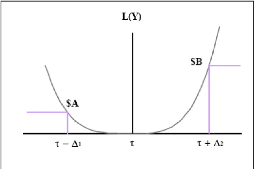
A non-symmetric step function and a corresponding continuous loss function are shown in Figure 1.
In this figure W'1and W'2are the lower and the upper specification limits, respectively, and A
and B represent the cost of correcting and/or replacing a unit that measures at or beyond the specification limits (i.e. a nonconforming unit).We assume that the continuous loss function has the following properties:
i) "(W'1) A, ii) "(W'2) B, and iii) "cc(y)!0for all - < y < +. The first two properties stem from the fact that the continuous loss function needs to agree with the step function at the given specification limits, while the last property holds because we assume that the loss function is
convex everywhere. We determine the values of k2, k3, and k4 to satisfy these properties. At the
specification limits we have
2 3 4
1 2 1 3 1 4 1
(W ' ) A k ' ' k k '
" (3)
2 3 4
2 2 2 3 2 4 2
(W ' ) B k ' ' 'k k
Figure 1: A non-symmetric loss function
By solving equations (3) and (4) for k2 and k3 in term of k4 we get
21
2 2 3 1 2 1 4
1 1 2
2
1 1
B A
k k
§ ·
¨ ¸§ ' ·
¨ ¸¨ ' ' ' ¸
' ' '
¨ ¸© ¹
¨ ' ¸
© ¹
(5)
2 1
3 3 2 2 4
1 2 1 2 2
2
1 1
B A
k k
§ ·
¨ ¸§ §' · ·
¨ ' ¸¨¨ ¨ ' ¸ ¸¸
' ' ' '
¨ ¸© © ¹ ¹
¨ ' ¸
© ¹
(6)
It is clear that the coefficients are not uniquely specified at this point. For any value of k4,
however, the corresponding values of k2 and k3 can be determined using these equations. We now
consider the last property, i.e.,"cc(y)!0,f yf. From equation (2) it follows that
2
2 3 4
( )y 2k 6 (k y W) 12 (k y W)
cc
" (7)
which can be rearranged in the form
2 2
4 3 4 2 3 4
( )y (12 )k y (6k 24Wk y) (2k 6Wk 12W k )
cc
" (8)
This is the well-known quadratic formg(y) ay2byc, and it can be easily shown that in order to
have g(y)!0for all values of y we must have a > 0 andb24ac. It follows that for "cc(y)to be
positive everywhere we must have 12k4 !0and 2 2
3 4 4 2 3 4
equivalently, we must have k4 !0 and 32 2 4
3 8
k k
k . Substituting for k2 and k3 from equations (5)
and (6), the latter expression reduces to
2 2 2 2 2 3
( ) 8 2
2
1 2 1 2 1 2 1
4 2 3 2 2 2 2 ( ) ( )
2 2 ( 2 2) 8 1 2 1 1 2 2 0
1 2 4
4 2 2 3 2 4 6 2 4 4 2
2 1 2 1 2 2 2 1 2 1 2
k
A B
B A B AB A
k
ª ' ' §' ' ' ' ' ·º
« ¨ ¸»
« ¨ ' ¸»
¨ ¸
'
« © ¹»
¬ ¼
ª§ · § ' ' ' ' ' ·º ª º
«¨ ¸ ' ' ¨ ¸» « »
«¨¨ ¸¸ ¨¨ ¸¸» « »
' ' ' ' ' ' ' ' ' ' '
«© ¹ © ¹» «¬ ¼»
¬ ¼
(9)
Any positive value of k4 that satisfies this inequality leads to "cc(y)!0everywhere. This typically
(but not always) leads to a range of allowable values fork4, and we can select the value of k4 within
this range. The corresponding values of k2 and k3 are then determined using equations (5) and (6),
respectively. The shape of the loss function depends on the value of k4 that we select within this
range, and for this reason we refer to k4 as the shape parameter.
Now let’s assume further that'1 '2 '. In this case equations (5) and (6) reduce to
2
2 2 4
2
A B
k ' k
' (10)
3 2 3
B A
k
' (11)
We observe that in this case the value of k3 does not depend on k4 and it is uniquely determined in
equation (11), but the value of k2 still depends onk4. Similarly by letting '1 '2 ' equation (9)
reduces to
2 4 2
4 4 4
3 ( )
(2 ) ( ) 0
8 2
B A
k A B k
'
' (12)
and any positive value of k4 that satisfies this inequality leads to "cc(y)!0 everywhere.
2.2. The Symmetric Case
A symmetric loss function is the special case of what we discussed above with'1 '2 ' and B =
A. In this case equations (10) and (11) reduce to
2
2 2 4
A
k ' k
' (13)
3 3 0
2
A A
k
and equation (12) reduces to
4 2
4 4
(2' )k (2 )A k 0 (15)
It follows that 0 < k4 <
4 '
A
. It is interesting to observe the form of the loss function at the two
extreme values ofk4. At k4 = 0 from equation (13) we have k2 =
2 '
A
, and the loss function reduces
to the well-known quadratic loss function of the form ( ) 2 ( W)2
' y
A y
" , while at 4 4
'
A
k 4 we have
2
k = 0, and the loss function reduces to 4
4 ( )
)
( W
' y
A y
" .
2.3. Numerical Examples
We present two numerical examples to illustrate the family of loss functions represented by this quartic function.
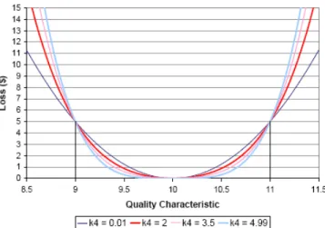
Example 1. We assume that the target value for a quality characteristic of interest is IJ = 10 and its
specification limits are 10 ± 1 (i.e., '1 '2 1). We also assume that the cost for repairing or
replacing a nonconforming unit is $5 at either specification limit, i.e., the loss function is symmetric withA = 5. It follows from equations (14) and (15) that k3 = 0 andk4(0,5), and the corresponding
value of k2 is determined using equation (13). In Figure (2) we present four profiles of this quartic
loss function based on four different values of k4 = 0.01, 2.0, 3.5, and 4.99. The associated values
of k2 are 4.99, 3.00, 1.50, and 0.01, respectively.
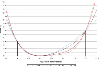
Example 2. We again assume that the target value is IJ = 10, but the lower and upper specification
limits are assumed to be 9 and 12, respectively, i.e., '1 = 1 and '2 = 2. Further we assume that the
associated costs are A = 4 and B = 7. From equation (9) we have k4(0.085, 1.047), and the
corresponding values of k2 and k3 are determined using equations (5) and (6), respectively. Again
we present four profiles of the corresponding quartic loss function based on four different values of
4
k = 0.15, 0.4, 0.8, and 1. From equation (5) the associated values of k2 are 2.95, 2.45, 1.65, and
1.25, respectively, and from equation (6) the associated values of k3 are -.9, -1.15, -1.55, and -1.75,
respectively. The corresponding loss function profiles are shown in Figure 3.
Figure 3: A family of asymmetric quartic loss functions corresponding to Example 2
Discussion. In Figures 2 and 3 we observe that as we change the value of k4 within its range, the shape of the corresponding loss function changes in a systemic way. For the symmetric case, when
4
k is at its lower limit "(y) reduces to a quadratic loss function, and in either case as we increase
the value of k4 the shape of this function within the specification limits becomes closer to the form
of the conventional step function. Outside of the specification limits, however, the quartic function
increases rapidly (specially for the larger values ofk4), and it does not resemble the corresponding
step function at all, as mentioned earlier. Thus, by selecting an appropriate value for this parameter the problem solver can determine the shape of the loss function and its degree of similarity to either the quadratic loss function or the step function within the specification limits. In either case, however, special attention must be paid to the value of the function outside of the specification limits and its impact on the subsequent analysis. See Fathi (1990) for a discussion of this issue in the context of the quadratic loss function.
3. EXPECTED LOSS PER UNIT
Because the quality characteristic Y varies from unit to unit and from time to time, it is customary to represent its variation by a probability distribution function. Let f (y) be the probability density function of Y. In many industrial applications we need to determine the corresponding expected value of loss per unit, which can be written as
[ ( )] ( ) ( )
E Y y f y dy
f
f
³
" " (16)
By substituting the quartic loss function of equation (2) in equation (16) we have
2 3 4
2 3 4
2 3 4
2 3 4
2 2 2 3 2
2 3 4
[ ( )] { ( ) ( ) ( ) } ( )
[( ) ( )] ( ) [( ) ( )] ( ) [( ) ( )] ( )
[ ( ) ] [ 3 ( ) ( ) ] [ 4 ( ) 6
Y Y Y Y Y Y
Y Y Y Y Y Y Y Y Y Y
E Y k y k y k y f y dy
k y f y dy k y f y dy k y f y dy
k k k
W W W
P P W P P W P P W
V P W I V P W P W M I P W V
f
f
f f f
f f f
³
³
³
³
"
2 4
(PY W) (PY W) ] (17)
where PY is the mean of Y, VY2 is the variance of Y , and IY and MY are the third and the fourth
moments of Y about its mean, respectively. For the symmetric case we have k3 = 0, and equation
(17) reduces to
2 2 2 2 4
2 4
[ ( )] [ Y ( Y ) ] [ Y 4 Y( Y ) 6 Y( Y ) ( Y ) ]
E "Y k V P W k M I P W V P W P W (18)
Table 1: Expected loss per unit
Example 1. (continued) To observe the impact of changing the shape parameter k4 on the expected
loss per unit we calculate this value in the context of example 1. We assume that Y has a normal
distribution with mean ȝY = 10, and with variance Vy2 0.2. It follows thatIY 0, 3 0.12
4 Y Y V
M .
We use equation (18) to determine the expected loss per unit at three different values of k4 within its
range, and the results are shown in Table 1. For comparison we also include the expected loss per
unit for the corresponding quadratic loss function (i.e., when k4 = 0) and for the conventional step
function. We observe that as we increase the value of k4, the corresponding value of the expected
loss per unit becomes smaller, i.e., it becomes closer to the value obtained via the step function.
4. THE PARAMETER DESIGN MODEL
Following the pioneering work of Taguchi (1978), in the past two decades the subject of robust design of manufactured products and/or manufacturing processes has received considerable attention in the open literature. See, for example, Box (1988), Fathi (1997), Fowlkers and Creveling (1997), Leon et al. (1987), and Phadke (1989). Most of these articles are based on the premise that the quality loss is measured by a quadratic function, although Fathi and Palko (2001) discuss the problem in the context of the conventional step function as well. In this section we study this problem using a quartic loss function. Employing the quartic function in this context provides a degree of freedom for choosing the shape of the loss function between the two extremes represented by the quadratic loss function and the corresponding step function, respectively, as discussed earlier. It also facilitates the analysis of the problem when the loss function is non-symmetric. LetX = (X1, X2, . . . , Xn) be a vector of design variables (components) for a manufactured product or
a manufacturing process, and let Y = h(X1, X2, . . . , Xn) represent a quality characteristic of interest.
We assume that the functional relationship h (i.e., the transfer function) is available in closed form, or at least it could be well approximated, and that it is continuous and differentiable everywhere.
We also assume that X1 through Xn are random variables with known probability distribution
functions and with respective nominal values ȝ1 through ȝn. It follows that Y = h(X1, X2, . . . , Xn) is
also a random variable whose probability density function and its associated parameters depend on
the form of the transfer function h and on the probability density functions of X1through Xn. In
We define the parameter design problem to be the problem of determining an optimal set of values
for ȝ1 through ȝn so as to minimize the expected loss associated with the quality characteristic Y.
Certain constraints pertaining to the technical requirements of the product, its manufacturing limitations, and its processing costs may also be applicable, and these constraints define the feasible
region for ȝ1 through ȝn. Assuming that the loss per unit is represented by a quartic function as
discussed earlier, the problem can be expressed as the following mathematical programming model Minimize
2 2 2 3
2 3
2 2 4
4
[( ( )] [ ( ) ] [ 3 ( ) ( ) ]
[ 4 ( ) 6 ( ) ( ) ]
Y Y Y Y Y Y Y Y Y Y Y Y
E Y k k
k
V P W I V P W P W
M I P W V P W P W
"
subject to (ȝ1,ȝ2, . . . , ȝn)
Mwhere
P
Y and VY2 are the mean and variance of Y , IYand MY are the third and fourth moments ofY about its mean, respectively, and ȝ1 through ȝn are the decision variables. The set M represents the
set of feasible values for ȝ1 through ȝn, and it includes all pertinent constraints.
Obviously the value of
P
Y, 2Y
V , IY, and MYdepend on the design parameters ȝ1 through ȝn.
However, the exact form of the functional relationship between these moments of Y and the
parameters ȝ1through ȝn may be difficult to obtain in closed forms (in some cases it may even be
impossible do so). Tukey (1957) uses the Taylor series expansion of the function h about the point ȝ
= (ȝ1,ȝ2, . . . , ȝn) to approximate these values. In this derivation Tukey assumes that X1, X2, . . . , Xn
are independent random variables with respective means ȝ1 through ȝn and respective variances
2 1
V through Vn2. Their respective skewness and kurtosis coefficients are defined as
2 3 2) ( i Y i V I
J and
2 2 ) ( i Y i V M
* for i = 1 to n. The corresponding formulas are
2 3 4 2 2
1 2
1 1 1 1
( , ,..., )
2 6 24 4
Y h n ihii i ihiii i i ihiiii i i i jhiijj i j
P | P P P
¦
V¦
J V¦
*V¦
V V (19)2 2 2 3 1 4 1 2 4 2 2 2
( 1) ( )
3 4
Y ihi i ih hi ii i i ih hi iii i i ihii i i i j h hi ijj hij h hiij j i j
V |
¦
V¦
J V¦
*V¦
* V¦
V V(20)
3 3 3 2 ( 1) 4 6 2 2
2
Y ihi i i ih hi ii i i i jh h hi j ij i j
I |
¦
J V¦
* V¦
V V (21)4 4 2 2
( 3) 3( )
Y ihi i i Y
M |
¦
* V V (22)where all summations are from 1 to n, and n
i i
x h h P,P2,...,P
w w , 1 2. 2 , ,..., 2 n ii i h h
x P P P
w
w ,
1 2
2
, ,..., n ij
i j
h h
x x P P P
w
w w , etc. Note that in the above expressions we reproduce the formulas up to the
include the terms of order ı5. In the numerical experiments that we carried out, we observed that
inclusion of the 5th order terms did not have a significant impact on the subsequent analysis of the
corresponding parameter design model, while the additional computational effort was exhaustive.
Needless to say that in other applications the situation may be different and inclusion of the 5th order
terms might prove to be significant.
In these formulas the values of
P
Y,T
Y2, IY, and MY are expressed as functions of ȝ= (ȝ1,ȝ2, . . . , ȝn), i.e., ȝY (ȝ),2
( )
Y
ȝ
T
, IY( )ȝ and MY( )ȝ , respectively. If we use these expressions in themathematical programming model discussed above we obtain the following model that we refer to
as the Parameter Design Model (PDM): find ȝ1 through ȝnto
^
`
^
` ^
`
^
`
^
` ^
`
2 3
2 2
2 3
2 4
2 4
Minimize
[( ( )] [ ( ) ( ) ] [ ( ) 3 ( ) ( ) ( ) ]
[ ( ) 4 ( ) ( ) 6 ( ) ( ) ( ) ]
Y Y Y Y Y Y
Y Y Y Y Y Y
E Y k k
k
V P W I V P W P W
M I P W V P W P W
" ȝ ȝ ȝ ȝ ȝ ȝ
ȝ ȝ ȝ ȝ ȝ ȝ
2 3 4 2 2
subject to
1 1 1 1
( ) (
2 6 24 4
Y h ihii i ihiii i ihiiii i i i jhiijj i j
P ȝ ȝ)
¦
V¦
J¦
*V¦
V V2( 2 2 3 1 4 1 2( 1) 4 ( 2 ) 2 2
3 4
Y ihi i ih hi ii i i ih hi iii i i ihii i i i j h hi ijj hij h hiij j i j
V ȝ)
¦
V¦
J V¦
*V¦
* V¦
V V3 3 3 2 4 2 2
( ( 1) 6
2
Y ihi i i ih hi ii i i i jh h hi j ij i j
I ȝ)
¦
J V¦
* V¦
V V4 4 2 2
))
( ( 3) 3( ( ,
Y ihi i i Y
M ȝ)
¦
* V V ȝ ȝ
MThis model is a nonlinear constrained optimization problem and it can be solved using appropriate nonlinear programming (NLP) algorithms. For a comprehensive discussion of NLP algorithms see Bazaraa and Shetty (1979).
4.1. A Case Study
To further illustrate this model and to demonstrate that it is mathematically tractable we briefly describe a case study that we adopt from Fathi (1997) with slight modifications. This case study pertains to the design of a coil spring. The performance characteristic of interest in this case is the deflection of the coil spring and our objective here is to demonstrate how the functional profile of the corresponding quartic loss function affects its optimal design. For the case of a symmetric function we also compare the results with those obtained via a quadratic loss function.
The Problem Statement. We consider a coil spring loaded in tension or compression. We adopt the following notation and data from Fathi (1997).
Shear modulus G = 1.15 × 10⁷ (lb/in2)
Weight density of a spring material V = 0.285 (lb/in3)
Mass density of the spring material ȡ = V
g = 7.38342 × 10
-4 (lb sec2/in4)
Deflection along the axis of the spring į (in) Shear stress S (lb/in2) Frequency of surge waves Ȧ (Hz) Applied load P (lbs)
Deflectionį is the performance characteristic of interest with a desired target value of 0.5 inches
when a load of P = 1000 lbs is applied. The shear stress S and the frequency of surge waves Ȧ are
the technical characteristics of the coil spring whose values should be within certain limits for proper function of the product. The following parameters represent the design variables in this problem:
Wire diameter: d (in.)
Coil diameter: D (in.)
Number of active coils: N
We consider d, D, and N to be pairwise independent normally distributed random variables with
respective means ȝd,ȝD,ȝN , and with respective variances Vd2 ,VD2, and VN2. We assume that ıd =
0.006, ıD = 0.025, ıN = 0.2, and since all random variables are normally distributed we have Ȗd = ȖD
= ȖN = 0, and*d *D *N 3. In the context of this problem ȝd, ȝD, and ȝN are the decision
variables, and we would like to determine their optimal set points so as to minimize the expected loss per unit.
The deflection of the spring under an applied load of 1000 lbs (which is the performance characteristic of interest in this case) can be written as:
3
4
( , , )
1437.5 D N h D N d
d
G (23)
The following requirements define the feasible domain for the design variables: i) the maximum
allowable shear stress in the spring is 80, 000 lb/in2, ii) the frequency of surge waves must be at
least 100 Hz, and iii) the outer diameter of the coil spring is required to be no bigger than 2.5 inches. These requirements can be written as the following constraints.
3 2
636.62 (4 ) 1566.084
80, 000
( )
D D d
d D d d
d
(24)
2
14045.1 100 d
D N t (25)
2.5
Table 2: Results for the symmetric loss function
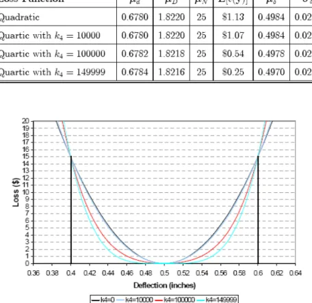
Figure 4: Family of the symmetric loss functions Finally, we have the following explicit bounds on the decision variables. 0.2 ≤ μd ≤ 0.8
0.9 ≤ μD ≤ 2 (27)
2 ≤ μN ≤ 25
These constraints define the feasible region M, and the corresponding parameter design model (PDM) can be constructed using the transfer function (23) along with an appropriate loss function for the performance characteristic δ. We carry out this analysis with two different loss functions for
δ: a symmetric loss function and a non-symmetric loss function.
Symmetric loss function We assume that the specification limits for δ are 0.5 ± 0.1, and the loss at either limit is $15 (i.e., A = B = 15). From equations (14) and (15) for the symmetric quartic loss function we have k3 = 0, k4
∈
(0, 150000), and for each value of k4 the associated value of k2 can be determined using equation (13). We solve the corresponding PDM at three different values of the shape parameter k4 = 10,000, 100,000, and 149,999. The associated values of k2 are 1400, 500, and 0.01 respectively, and the corresponding loss function profiles are depicted in Figure 4. We also solve the problem using the corresponding quadratic loss function. Respective optimal solutions and their associated values are reported in Table 2. We observe that in this case the optimal solution for the problem does not change much as we change the value of the shape parameter k4, although the corresponding value of the objective function (i.e., the expected loss per unit) gets smaller as we increase the value of k4. This observation is consistent with those reported in Fathi and Palko (2001).Table 3: Results for the non-symmetric loss function
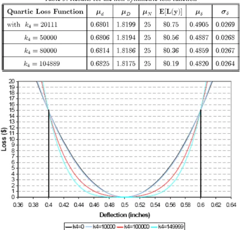
Figure 5: Family of non-symmetric loss functions
Non-symmetric loss function This is similar to the above case with the same specification limits, but we assume that A = $5 while B = $20, i.e., the corresponding loss function is non-symmetric,
although we still have ¨1 =¨2 = 0.1. From equations (11) and (12) for the non-symmetric loss
function we have k3 = 7500 and k4 (20110.4, 104889.6). For each value of k4 in this range the
corresponding value of k2 can be determined using equation (10). We solve the parameter design
problem with four different values of the shape parameter k4 = 20111, 50000, 80000, and 104889.
The associated values of k2 are 1048.9, 750.0, 450.0, and 201.1, respectively, and the corresponding
loss function profiles are depicted in Figure 5. Respective optimal solutions and their associated values are summarized in Table 3.
We observe that at k4 = 20111 the optimal value of the design variables are slightly different from
those obtained in the symmetric case above, and the corresponding value of ȝį is slightly below its
target value of 0.5. As we increase the value of the shape parameter k4 this difference gets larger
and the corresponding value of ȝį moves further below its target value. This is a natural and
expected consequence of the non-symmetric loss as depicted by the quartic loss function.
5. CONCLUDING REMARKS
The quartic function that we propose here provides a unifying format for approximating both symmetric and non-symmetric continuous quality loss functions. The choice of its shape parameter provides the user with a degree of flexibility to select its profile, and the corresponding expected
loss per unit can be easily determined. As a result the quartic loss function can be adopted in various applications such as in the parameter design problem that we discussed above. Note that when we use a quadratic loss function it is significantly more difficult to deal with the asymmetric form in the context of the parameter design problem since the corresponding nonlinear programming model is not so easy to obtain or solve.
Similar to the quadratic loss function, however, this function has the drawback that it increases rapidly outside of the specification limits. Therefore special attention must be paid to its use if the quality characteristic is likely to be outside of these limits, and appropriate measures should be introduced to eliminate any undesirable impact that this feature might have. A comprehensive discussion of this issue in the context of the quadratic loss function is given in Fathi (1990) and we are presently investigating this subject in the context of the quartic loss function.
Acknowledgement The work of the first author is supported by the NSF grant DMI-0321635, which is gratefully acknowledged.
REFERENCES
[1] Bazaraa Mokhtar S., Shetty C.M. (1979), Nonlinear programming, theory and algorithm, Wiley. [2] Box G.E.P. (1988), Signal-to-noise ratio, performance criteria, and transformations; Technometrics 30;
1-17.
[3] Evans David H. (1975), Statistical tolerancing: The state of the art part II. methods for estimating moments; Journal of Quality Technology 7; 1-12.
[4] Fathi Y. (1990), Producer-consumer tolerances; Journal of Quality Technology 22; 138-145.
[5] Fathi Y. (1997), A linear approximation model for the parameter design problem; European Journal of Operational Research 97; 561-570.
[6] ––––, Palko D. (2001), A mathematical model and a heuristic procedure for the robust design problem with high-low tolerances; IIE Transactions 33; 1121-1127.
[7] Fowlkers William Y., Creveling Clyde M. (1997), Engineering Methods for Robust Product Design: Using Taguchi Methods in Technology and Product Development, Addison-Wesley.
[8] Leon R., Shoemaker A.C., Kackar R.N. (1987), Performance measures independent of adjustment (with discussions); Technometrics 29; 253-285.
[9] Leung Bartholomew P. K., Spiring Fred A. (2002), The inverted Beta loss function: properties and applications; IIE Transactions 34; 1101-1109.
[10] Phadke Madhav S. (1989), Quality engineering using robust design, Prentice Hall.
[11] Spiring F.A. (1993), The reflected normal loss function; Canadian Journal of Statistics 21(3); 321-330.
[12] Spiring F.A., Yeung A.S. (1998), A general class of loss functions with industrial applications; Journal of Quality Technology 30(2); 152-162.
[13] Sun F. B., Laramee J. Y., Ramberg J.S. (1996), On Spiring’s normal loss function; Canadian Journal of Statistics 24(2); 241-249.
[14] Taguchi G. (1978), Off-line and on-line quality control system; International Conference on Quality Control, Tokyo, Japan.
[15] ––––– (1986), Introduction to Quality Engineering, Asian Productivity Organization.
[16] –––––, Elsayed Elsayeda A., Hsiang Thomas (1989), Quality engineering in production systems, McGraw-Hill.
[17] Tukey John W. (1957), Propagation of errors, fluctuations and tolerances, No. 1: Basic generalized formulas; Technical Report No. 10, Princeton University, Princeton, NJ.