Open Journal Systems

(1)

ORIGINAL ARTICLE

Decomposing the Slutsky Decomposition for the First Time in a

Cen-tury

Kazuyuki Sasakura1

Professor, Faculty of Political Science and Economics, Waseda University, Japan

Abstract: The Slutsky decomposition is a mathematical formula which has been used for a very long time in eco-nomics to analyze how the demand for a good changes when its price goes up. Such a change in the demand is called the price effect. Most people will expect a decrease in the demand in response to a rise in the price. In other words, they will have a downward sloping demand curve in mind. Indeed they are right in usual cases. In terms of economics it is said that the price effect is usually negative. But why? The Slutsky decomposition gives a correct answer to this question by decomposing the price effect into the substitution effect and the income effect. It is al-ready known that the substitution effect is always negative, while the income effect is also negative if a good un-der consiun-deration is “normal.” Since the sum of the two effects equals the price effect, it can be concluded that a demand for the good decreases when its price goes up, or the demand curve is downward sloping, in a “normal” situation. The Slutsky decomposition is so elegant and powerful that there would not be any economist who stud-ies consumer behavior without mentioning it. Then, is there other decomposition than the Slutsky? This paper in-troduces a new one which decomposes the price effect into the unit-elasticity effect and the ratio effect. The unit-elasticity effect means by how much the demand decreases in response to a rise in the price with the ex-penditure on it as fixed. The ratio effect means by how much the demand changes due to a change in the ratio of the expenditure on it to total income. The former effect is always negative, but the latter effect may be positive even in a “normal” situation. It is shown that a new decomposition is obtained by decomposing the Slutsky de-composition.

Keywords:The Slutsky decomposition; A new decomposition; A Giffen good; Hicks’s Value and Capital

1. Introduction

What comes to your mind first when you hear the term economics? It must be supply and demand. Certainly economics is based on the analysis of supply and demand. If you learned economics, it may be supply and demand curves on a plane. Supply or a supply curve is not directly related to ordinary people because it describes a firm which is planning how much to produce to each price of its good. Economics teaches us that the supply of a good always increases in re-sponse to a rise in the price. It means that a supply curve is always upward sloping.

On the other hand, demand or a demand curve is directly related to ordinary people because they like to buy goods or have to buy some in a daily life. Consumer theory is a field of economics in which how much such a person

1_{Part of this paper was presented at BIT’s 4th Annual Global Congress of Knowledge Economy 2017 held in}

Qing-dao, China. I appreciate a lot of kindness from Ms. Wendy Wang as its coordinator.

This is an open-access article distributed under the terms of the Creative Commons Attribution Unported License

(http://creativecommons.org/licenses/by-nc/4.0/), which permits unrestricted use, distribution, and reproduction in any medium, provided the original work is properly cited.

(2)

2 | Kazuyuki Sasakura. Finance and Market

called a consumer decides to buy to each price of a good is analyzed. Needless to say, a demand curve is a mathematical representation of the behavior of a consumer. The Slutsky equation is a mathematical tool to examine the response of the quantity demanded of a good to a change in its price. It was proposed about a century ago by Slutsky [1], a Russian mathematician and statistician. Since then there would have been no economists in consumer theory who did not rely on it in their research. Textbooks of economics explaining consumer behavior always use it explicitly or implicitly. It is no exaggeration to say that it is still the only and unassailable base in consumer theory. As Barnett [2] said, “Publishing this contribution alone would have guaranteed Slutsky a permanent place in the pantheon of authors of classic articles on economic theory.” (p. 44) 2

The Slutsky equation decomposes the price effect into the substitution effect and the income effect. The price ef-fect here literally means by how much the quantity demanded of a good under consideration changes when its own price rises by a unit with income of a consumer and prices of other goods fixed. Graphically it corresponds to the slope of a demand curve. As is easily imagined, the price effect is usually negative since a demand curve is usually drawn as a downward sloping curve on a plane. But why? The answer all economists give with confidence to this question is be-cause the sum of the substitution effect and the income effect is negative.

The substitution effect means by how much the quantity demanded decreases if the utility of a consumer is held at the same level even after the price rises. Since the marginal rate of substitution between two goods is assumed to be decreasing, the consumer chooses less quantity of the good in question with a relatively high price and more quantity of the other good with a relatively cheap price in such a situation. Thus, the substitution effect is always negative. The in-come effect means by how much the quantity demanded changes in response to a fall in real inin-come (or the purchasing power) which comes from the rise in the price. It may be negative, positive, or zero. A good with a negative income effect is called a normal good, while a good with a positive income effect an inferior good. As the appellation suggests, the quantity demanded of a normal good increases with income of a consumer with all prices fixed, while the quantity of an inferior good decreases under the same circumstances. Such a decomposition of the price effect is called the Slut-sky decomposition. Since the SlutSlut-sky decomposition based on the SlutSlut-sky equation is perfectly elegant in terms of both mathematics and economics, economists as well as economics students have made it a rule to study a consumer decision along the line of it.

Nevertheless, it can also be said that the Slutsky decomposition leads simply to a confirmation of our intuition that the demand for a normal good must decrease when its price goes up, or in other words, the demand curve of a normal good is downward sloping. Such a proposition itself deserves to be respected as a result of scientific reasoning, but it may appear to be a matter of course from an ordinary viewpoint.

A conventional way which has been long used by economists to show the usefulness of the Slutsky decomposition is the application of it to an inferior good. As said above, an inferior good is one with a positive income effect. For in-stance, if corn and beef are respectively an inferior good and a normal good for some consumer, it means that the de-mand for corn decreases and that for beef increases with her income under the condition that the prices of both goods remain unchanged. In such a case the Slutsky decomposition is expressed as the sum of a negative term and a positive term. If the former dominates the latter, then such an inferior good has a downward sloping demand curve as a normal good does. But if the latter dominates the former, the price effect becomes positive, which implies an upward sloping demand curve! An inferior good with an upward sloping demand curve is called a Giffen good after Scottish economist Robert Giffen. Indeed it has been examined by quite a few researchers either theoretically or empirically. And the Slut-sky decomposition has been relied on to explain why a Giffen good can exist. But it should be said at the same time that a Giffen good is a very special kind of good both theoretically and empirically. Thus, it is a little strange to me to argue

(3)

that the Slutsky decomposition is useful because it can explain a Giffen good.

Recently I have found a way to decompose the Slutsky decomposition further as in Sasakura [4]. According to it, the price effect can be decomposed into three effects, i.e., the unit-elasticity effect, the transfer effect, and the substitu-tion effect. The unit-elasticity effect means by how much the quantity demanded of a good under considerasubstitu-tion de-creases if the expenditure on it remains unchanged even after its own price rises. So it is always negative. The transfer effect means by how much the demand for the other good is transferred to that for the good under consideration due to a fall in real income (or the purchasing power) which comes from the rise in the price. So it is positive (negative) if the other good is normal (inferior). The substitution effect is the same as that in the Slutsky decomposition. So it is always negative. Such a decomposition can also be expressed as the sum of two effects, i.e., the unit-elasticity effect and the ratio effect. To avoid ambiguity, a “new decomposition” will refer to this two-effect decomposition. The ratio effect is the sum of the transfer effect and the substitution effect. It is positive (negative, zero) if the ratio of the expenditure on the good to total income increases (decreases, remains unchanged) when the price goes up. Thus, the price effect may be decomposed into two terms with opposite signs even in the case of a normal good. It should also be noticed that the Slutsky decomposition is included in the above-mentioned three-effect decomposition since the sum of the unit-elasticity effect and the transfer effect is equal to the income effect.

This paper is organized as follows. Sections 2 and 3 respectively explain the Sltusky decomposition and a new decomposition using mathematical expressions as well as figures. Section 4 compares the two decompositions and gives examples of application using the CRRA utility function and the case of a Giffen good. Section 5 concludes by making a “historical” remark about Hicks’s Value and Capital.

2. The Slutsky Decomposition

Consider a consumer who decides to buy good 1 and good 2 under the budget constraint 𝑝₁𝑞₁+ 𝑝₂𝑞₂= 𝑦, where 𝑝₁ and 𝑞1are respectively the price and quantity of good 1, 𝑝2 and 𝑞2are the price and quantity of good 2, and 𝑦 is in-come. The objective of the consumer is to maximize her utility described by a utility function 𝑣 = 𝑢(𝑞1, 𝑞2) with 𝑝1,

𝑝2, and 𝑦 as given. Then, she tries to solve the following utility maximization problem:

max𝑞₁,𝑞₂𝑢(𝑞1, 𝑞2) subject to 𝑝1𝑞1+ 𝑝2𝑞2= 𝑦,

where 𝑢₁(𝑞₁, 𝑞₂) > 0, 𝑢₂(𝑞₁, 𝑞₂) > 0, and |𝑈| ≡ −𝑢₂2𝑢₁₁+ 2𝑢₁𝑢₂𝑢₁₂− 𝑢₁2𝑢₂₂> 0. The positivity of determinant

|𝑈| assures that the marginal rate of substitution between goods 1 and 2 is decreasing. As a solution to this problem, the Slutsky equation can be written as follows:

𝜕𝑞₁ 𝜕𝑝₁|_𝑝

2,𝑦=const ⏟ price effect

= 𝜕𝑞1 𝜕𝑝₁|_𝑝

2,𝑣=const ⏟ substitution effect

−𝑞1𝜕𝑞_𝜕𝑦1|

𝑝₁,𝑝₂=const ⏟

income effect

, (1)

where 𝜕𝑞_𝜕𝑝1

1|𝑝₂,𝑣=const= − 𝑢₁𝑢₂2

𝑝1|𝑈|< 0, −𝑞1 𝜕𝑞₁

𝜕𝑦|_𝑝

1,𝑝2=const

= −𝑞1𝑢1(𝑢2𝑢_𝑝12−𝑢1𝑢22)

1|𝑈| < 0, and all partial derivatives and

𝑞1 are evaluated at an optimal point. The Slutsky equation (1) shows that the price effect is decomposed into the sub-stitution effect and the income effect. This formula is called the Slutsky decomposition.

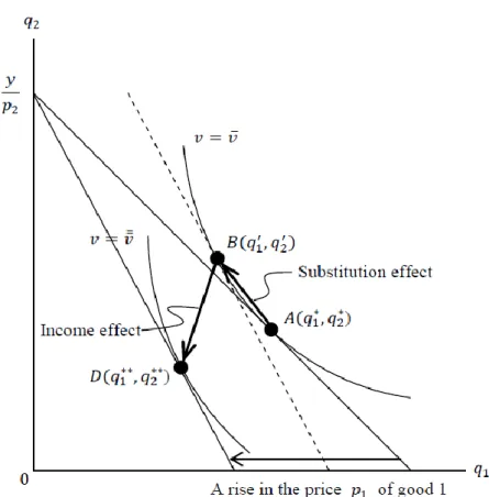
It is easy to understand the implication of the Slutsky decomposition by using Figure 1 in which both good 1 and good 2 are assumed to be normal. A downward sloping curve 𝑣 = 𝑢(𝑞1, 𝑞2) with constant 𝑣 is called an indifference curve, which implies combinations of goods 1 and 2 giving the same utility. In order to maximize her utility 𝑢(𝑞1, 𝑞2), she must choose a point at which an indifference curve is tangent to a budget line 𝑝₁𝑞₁+ 𝑝₂𝑞₂= 𝑦. Point 𝐴(𝑞₁∗, 𝑞₂∗) is an initial optimal point, at which indifference curve 𝑣̅ = 𝑢(𝑞1, 𝑞2) is tangent to an initial budget line. Thus, 𝑣̅ is a

(4)

Figure 1. The Slutsky Decomposition: The Case of a Normal Good

(5)

𝑝2 and y remain unchanged. What happens? First notice that a budget line rotates clockwise around the intercept

(0, 𝑦/𝑝2). Second find new optimal point 𝐷(𝑞1∗∗, 𝑞2∗∗) on the new budget line. As at point 𝐴(𝑞1∗, 𝑞2∗), new indifference curve 𝑣̿ = 𝑢(𝑞1, 𝑞2) contacts the budget line at point 𝐷(𝑞1∗∗, 𝑞2∗∗). Although 𝑣̿ is smaller than 𝑣̅, 𝑣̿ is a maximized utility, and 𝑞₁∗∗ is the demand for good 1 under the new circumstances.

As is obvious, a decrease in the demand for good 1 from 𝑞₁∗ to 𝑞₁∗∗ corresponds to the (negative) price effect in (1). The Slutsky decomposition divides such a change in demand from point 𝐴 to point 𝐷 into a change from point 𝐴 to point 𝐵 and that from point 𝐵 to point 𝐷. Point 𝐵(𝑞₁′, 𝑞₂′) lies on the same indifference curve as point 𝐴, but the slope of the indifference curve at point 𝐵 is the same as that of the new budget line which is steeper than that of the initial budget line. Thus, point 𝐵 is the one she chooses if she wants to enjoy the same utility as before the price goes up by substituting good 2 for good 1. It follows that 𝑞₁∗> 𝑞₁′ and 𝑞₂∗< 𝑞₂′. The decrease in the demand for good 1 from 𝑞₁∗ to 𝑞₁′ corresponds to the (always negative) substitution effect in (1). Now remember that she has income 𝑦 as her purchasing power. But after the price 𝑝₁ of good 1 rises by a unit, the purchasing power reduces to 𝑦 − 𝑞₁∗. In other words her real income decreases by 𝑞1∗. That is why the mathematical expression for the income effect in (1) in-cludes a coefficient −𝑞1. This decrease in real income shifts the dashed straight line contacting point 𝐵 downward to the new budget line on which new optimal point 𝐷 is located. Since both goods are normal, 𝑞₁∗∗< 𝑞₁′ and 𝑞₂∗∗< 𝑞₂′ as the figure shows. The decrease in the demand for good 1 from 𝑞1′ to 𝑞1∗∗ corresponds to the (negative) income ef-fect in (1).

Therefore, the price effect (𝑞1∗∗− 𝑞1∗) is decomposed into the substitution effect (𝑞1′− 𝑞1∗) and the income effect

(𝑞1∗∗− 𝑞1′). This is what the Slutsky equation has been telling us for a century.

3. A New Decomposition

The same price effect from point 𝐴 to point 𝐷 in Figure 1 can also be examined by solving the following utility maximization problem:

max𝜃𝑢(𝑞1, 𝑞2) subject to 𝑞1=𝜃𝑦_𝑝

1, 𝑞2=

(1−𝜃)𝑦

𝑝2 , 0 ≤ 𝜃 ≤ 1,

where 𝜃 is the ratio of the expenditure on good 1 to total income 𝑦. The two problems are mathematically equivalent, so the solutions to them are also just the same. The difference is only that the consumer maximizes her utility by calcu-lating the quantities of goods in the previous section and by adjusting the expenditure on goods in this section. But it makes a big difference about the decomposition of the price effect. In fact, as a solution to the above problem, the price effect can be decomposed as follows:

𝜕𝑞_𝜕𝑝1

1|_𝑝₂_,𝑦=const ⏟ price effect

= 𝜕𝑞1

𝜕𝑝1|_{𝑦,𝜃=const} ⏟ unit−elasticity effect

+𝑝2 𝑝1𝑞1

𝜕𝑞2 𝜕𝑦|_𝑝

1,𝑝2=const ⏟

transfer effect

+ 𝜕𝑞1

𝜕𝑝1|_𝑝₂_,𝑣=const ⏟ substitution effect

, (2)

where 𝜕𝑞1

𝜕𝑝₁|_{𝑦,𝜃=const}= − 𝑞1

𝑝₁< 0, 𝑝2

𝑝₁𝑞1 𝜕𝑞2

𝜕𝑦|_𝑝

1,𝑝2=const

=𝑝2

𝑝₁𝑞1

𝑢2(𝑢1𝑢12−𝑢2𝑢11)

𝑝₂|𝑈| > 0, and all partial derivatives and 𝑞1 are evaluated at an optimal point. Equation (2) tells us that the price effect is decomposed into the unit-elasticity effect, the transfer effect, and the substitution effect.

The unit-elasticity effect means by how much the demand for good 1 decreases if the expenditure 𝜃𝑦 on it does not change when the price 𝑝1 goes up. This effect is obtained at once by totally differentiating 𝑝1𝑞1= 𝜃𝑦 as

𝑑𝑞1/𝑑𝑝1= −𝑞1/𝑝1. Thus, it is always negative. “Unit-elasticity” refers to a situation in which a one percent rise in the price causes a one percent fall in the demand just as the result of the total differentiation shows. Also note that the de-mand for good 2 never changes under the same condition. This change is shown in Figure 2 as a horizontal arrow from point 𝐴(𝑞1∗, 𝑞2∗) on the initial budget line to point 𝐶(𝑞1′′, 𝑞2∗) on the new budget line.

(6)

The transfer effect in (2) resembles the income effect in (1), but they act in the opposite direction to the price effect. As said in the previous section, a unit rise in the price 𝑝₁ decreases the purchasing power by 𝑞₁ leading to a negative income effect. This also applies to good 2 at the same time. That is, the demand for good 2 also decreases by “𝑞1(∂𝑞2/ ∂𝑦)|𝑝1, 𝑝2= const” as an income effect on the side of good 2. But it is found from (2) that such a decrease in the demand for good 2 in turn is transferred to the demand for good 1. This is what the transfer effect means. It is posi-tive because good 2 is assumed to be a normal good. The substitution effect is the same as that in the Slutsky decompo-sition. Then, the price effect is the sum of two negative terms and one positive term.

Equation (2) reduces to

𝜕𝑞1 𝜕𝑝₁|_𝑝

2,𝑦=const

⏟

price effect

= 𝜕𝑞1

𝜕𝑝₁|_{𝑦,𝜃=const}

⏟

unit−elasticity effect

+

𝜕𝜃 𝜕𝑝1𝑦

𝑝₁

⏟

ratio effect

, (3)

where

𝜕𝜃 𝜕𝑝1𝑦

𝑝₁ = 𝑞₁ 𝑝₁

𝑢₂(𝑢₁𝑢₁₂−𝑢₂𝑢₁₁) 𝑝₂|𝑈| −

𝑢₁𝑢₂2

𝑝₁|𝑈|⋛ 0. Equation (3) shows that the price effect is also decomposed into the

unit-elasticity effect and the ratio effect, and this is what is called a “new decomposition” in this paper. The ratio effect means by how much the demand for good 1 changes due to a change in the ratio θ defined above. Comparing (2) and (3) reveals that the ratio effect is the sum of the transfer effect and the substitution effect. So it can take any sign. It is positive (negative, zero) if the expenditure on good 1 increases (decreases, remains unchanged) in response to a rise in the price 𝑝1 of good 1. In Figure 2 an arrow from point 𝐶(𝑞1′′, 𝑞2∗) to point 𝐷(𝑞1∗∗, 𝑞2∗∗) along the new budget line indicates this ratio effect. As is obvious, an increase in the demand for good 1 from 𝑞₁′′ to 𝑞₁∗∗ corresponds to a posi-tive ratio effect in (3). Such a change also means an increase in the ratio 𝜃 as a result of a rise in 𝑝₁.

In sum, according to a new decomposition, the price effect (𝑞1∗∗− 𝑞1∗) is decomposed into the unit-elasticity ef-fect (𝑞₁′′− 𝑞₁∗) and the ratio effect (𝑞₁∗∗− 𝑞₁′′). Figures 1 and 2 picture the same price effect about the same consumer. Now it turns out that equation (3) gives a decomposition quite different from the Slutsky.

4. The Relationship between the Two Decompositions

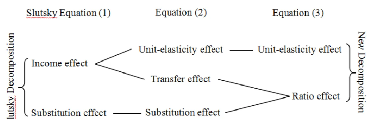
It is instructive to make clear the relationship between the Slutsky decomposition represented by (1) and a new decom-position represented by (3). It is summarized in Figure 3. The two decomdecom-positions are connected by equation (2) which decomposes the price effect into the three effects, i.e., unit-elasticity, transfer, and substitution effects. The Slutsky de-composition and a new dede-composition are both based on these three effects. In the Slutsky equation the unit-elasticity effect and the transfer effect constitute the income effect as the figure shows. The substitution effect is used in its origi-nal form. Thus, the price effect is aorigi-nalyzed in terms of the two effects, i.e., the income effect and the substitution effect. In the case of a normal good, both effects are negative. Thus, the price effect is negative, meaning that a corresponding demand curve is downward sloping.

On the other hand, the transfer effect and the substitution effect make the ratio effect in a new decomposition. The unit-elasticity effect is used as it stands. So the price effect is analyzed in terms of the different two effects, i.e., the unit-elasticity effect and the ratio effect. An interesting point is that the ratio effect may be positive even in the case of a normal good, though the unit-elasticity effect is always negative. Thus, the price effect may be the sum of two effects with opposite signs. Then, can the ratio be so large that the price effect becomes positive? The answer is no. This comes from the Slutsky decomposition which tells us that the income effect is negative if a good is normal. Thus, a maximal value the ratio effect takes never exceeds an absolute value of the unit-elasticity effect.

In order to calculate Equation (2) explicitly, let us take the following CRRA utility function as an example:

𝑣 = 𝑢(𝑞1, 𝑞2) = 𝑎𝑞1

1−𝛾

1−𝛾 + 𝑏

𝑞₂1−𝛾

(7)

Figure 3. The Relationship between the Slutsky Decomposition and a New Decomposition

Figure 4. Two Decompositions: The Case of a Giffen Good

Then, some manipulations show that

𝜕𝑞1

𝜕𝑝1|_𝑝₂_,𝑦=const ⏟ price effect

= −_1+𝑋1 _𝑝𝑦 1 2 ⏟ unit−elasticity effect

+ _(1+𝑋)𝑋 ₂_𝑝𝑦 12 ⏟ transfer effect

− 1 𝛾𝑋 (1+𝑋)2

𝑦 𝑝₁2 ⏟ substitution effect

= − 1+ 1 𝛾𝑋 (1+𝑋)2

𝑦

𝑝₁2< 0, （5）

where 𝑋 = (𝑏

𝑎)

1 𝛾₍𝑝1

𝑝2) 1 𝛾−1

(8)

8 | Kazuyuki Sasakura. Finance and Market 𝜕𝑞1

𝜕𝑝₁|_𝑝

2,𝑦=const ⏟ price effect = − 1 𝛾𝑋 (1+𝑋)2 𝑦 𝑝₁2 ⏟ substitution effect

−_(1+𝑋)1 ₂_𝑝𝑦 1 2 ⏟ income effect

, （6）

𝜕𝑞1

𝜕𝑝1|_𝑝₂_,𝑦=const ⏟ price effect

= −_1+𝑋1 _𝑝𝑦 1 2 ⏟ unit−elasticity effect − ( 1 𝛾−1) (1+𝑋)2 𝑦 𝑝₁2 ⏟ ratio effect

. （7）

According to Equation (7), the ratio effect is positive (negative, zero) if 𝛾 is greater than (smaller than, equal to) unity.

𝛾 is called the degree of the relative risk aversion, and the reciprocal of it is called the elasticity of substitution. It is known that when 𝛾 = 1, i.e., both the degree of the relative risk aversion and the elasticity of substitution equal one, utility function (4) can be replaced by the Cobb-Douglas-type utility function which is of the form 𝑣 = 𝑢(𝑞1, 𝑞2) =

𝑞1𝑎𝑞2𝑏. Good 1 is normal because the income effect is negative as Equation (6) shows. This implies that the price effect for good 1 is always negative.

A good with a positive price effect is called a Giffen good. It is a kind of inferior good. As said in the introduction, a Giffen good has often been analyzed using the Slutsky decomposition. It is also helpful to apply a new decomposition to such a case. Figure 4 compares them. Since 𝑞1∗< 𝑞1∗∗, good 1 is a Giffen good. As for the Slusky decomposition, a positive price effect comes from a very large income effect 𝑞₁∗∗− 𝑞₁′ > 0, though not shown by an arrow. As for a new decomposition, it comes from a very large ratio effect 𝑞₁∗∗− 𝑞₁′′ > 0 as shown by a long arrow from point 𝐶 to point

𝐷. Such a large ratio effect implies a larger transfer effect. It means in turn that good 1 is bought “at the sacrifice of good 2 despite a higher price of good 1. Such behavior seems to be pathological, and there are economists such as George Stigler, the Nobel laureate in economics 1982, who deny the existence of a Giffen good. But it cannot be denied at least theoretically.3

5. Concluding Remark

Anyone knows that economics is based on the analysis of supply and demand. It may be a matter of course. But it is interesting to know that Hicks [8] once said that “the theory of the equilibrium of the firm has been discussed almost ad nauseam in contemporary literature. In one sense, I have little to add to these discussions.” (p. 78) In his eyes the analy-sis of supply by the firm had already been completed at that time. Thus, it is consumer theory that he studied thoroughly using the Slutsky decomposition. In this final section, with the two decompositions introduced so far in mind I would like to make a “historical” comment on a figure in Hicks [8]_{, i.e., Figure 8 on page 31 of it. As far as I know, it is the}

figure that explained the Slutsky decomposition graphically for the first time in economics. Needless to say, Figure 1 of this paper traces back to the figure drawn by Hick. It goes without saying that the Slutsky decomposition would not have become so familiar in economics, were it not for such a figure.

Comparing Figure 8 of Hicks [8] and Figure 1 of this paper reveals that points 𝑄, 𝑃′, and 𝑃 in the former cor-respond respectively to points 𝐴, 𝐵, and 𝐷 in the latter with 𝑄 and 𝐴 as initial optimal points and 𝑃 and 𝐷 as new optimal points after a price rise.4 Since Hicks dealt with the case of a normal good, the substitution effect from point 𝑄 to point 𝑃′ along an indifference curve (𝐼₂) and the income effect from point 𝑃′ to point 𝑃 are both

3

For a theoretical example, Doi et al. [5] succeeded in providing a beautiful utility function leading to an upward sloping demand curve. For interesting empirical examples of Giffen goods, see Battalio et al. [6] and Jensen and Miller

[7]_. 4

In fact Hicks discussed the case of a price fall. Here I changed the direction of a price change, which never loses the essence of his explanations.

(9)

tive. Therefore the price effect is negative according to the Slutsky decomposition as in Figure 1.

Next, in order to apply a new decomposition to the same figure, draw a horizontal arrow from point 𝑄 to a new budget line (𝐿𝑀). And call the end of the arrow on the budget line 𝑄′. Then, 𝑄′ appears to be below 𝑃. It means that the ratio effect is negative in Hicks’s figure unlike in Figure 1. Or it can be said that the ratio effect is almost ze-ro because 𝑄′ and 𝑃 are very close. So I wonder what kind of utility function Hick had in mind while he was writing his book. Although he himself did not mention it, my conjecture is that it was something like the Cobb-Douglas-type utility function 𝑣 = 𝑞1𝑎𝑞2𝑏 as mentioned above. In other words, it would be utility function (4) with 𝛾 close to unity.5

Consumer theory has solid theoretical foundations thanks to the Slutsky equation or the Slutsky decomposition. But it proved that there is a different way. Then, as this paper showed part of it, the conventional Slutsky decomposition and a new decomposition help each other to analyze consumer behavior from a fresh point of view. The new evolution of consumer theory along such a line is to be expected.

References

1. Slutsky, Eugen E., 1915, “Sulla Teoria del Bilancio del Consumatore,” Giornale degli Economisti e Rivista di Statistica (now The Italian Economic Journal), Vol. 51, 1-26. Translated as “On the Theory of the Budget of the Consumer, ” in George J. Stigler and Kenneth E. Boulding, eds., 1952, Readings in Price Theory, Chicago: Richard D. Irwin, 27-56.

2. Barnett, Vincent, 2011, E.E. Slutsky as Economist and Mathematician: Crossing the Limits of Knowledge, London: Routledge. 3. Chipman, John S., and Jean-Sébastien Lenfant, 2002, “Slutsky’s 1915 Article: How It Came to Be Found and Interpreted,”

History of Political Economy, Vol. 34, 553-597.

4. Sasakura, Kazuyuki, 2016, “Slutsky Revisited: A New Decomposition of the Price Effect,” Italian Economic Journal, Vol. 2, 253-280.

5. Doi, Junko, Kazumichi Iwasa, and Koji Shimomura, 2009, “Giffen Behavior Independent of the Wealth Level,” Economic Theory, Vol. 41, 247-267.

6. Battalio, Raymond C., John H. Kagel, and Carl A. Kogut, 1991, “Experimental Confirmation of the Existence of a Giffen Good,” American Economic Review, Vol. 81, 961-970.

7. Jensen, Robert T., and Nolan H. Miller, 2008, “Giffen Behavior and Subsistence Consumption, ” American Economic Review, Vol. 98, 1553-1577.

8. Hicks, John R., 1939, Value and Capital: An Inquiry into Some Fundamental Principles of Economic Theory, Oxford: Claren-don Press. (2nd Edition, 1946.)

9. Krugman, Paul, and Robin Wells, 2009, Microeconomics, 2nd Edition, New York: Worth Publishers.

10. Nicholson, Walter, and Christopher Snyder, 2017, Microeconomic Theory: Basic Principles and Extensions, 12th Edition, Bos-ton, MA: Cengage Learning.

5_{A similar examination reveals at once the sign of the ratio effect in various figures explaining the Slutsky}

decom-position. For example, the ratio effect is negative in Figure 11-18 on page 295 of Krugman and Wells [9]. In Nicholson and Snyder [10] of 2017 the ratio effect is also negative in Figure 5.4 on page 147, but it is positive in Figure 5.3 on the preceding page. Figures 5.3 and 5.4 are the same as Figures 5.4 and 5.5 of the first edition of 1972! It shows how deeply