Advance Access publication 2017 July 6
Cross-correlating
Planck
tSZ with RCSLenS weak lensing: implications
for cosmology and AGN feedback
Alireza Hojjati,
1‹Tilman Tr¨oster,
1‹Joachim Harnois-D´eraps,
2Ian G. McCarthy,
3Ludovic van Waerbeke,
1,4Ami Choi,
2Thomas Erben,
5Catherine Heymans,
2Hendrik Hildebrandt,
5Gary Hinshaw,
1,4†
Yin-Zhe Ma,
6Lance Miller,
7Massimo Viola
8and Hideki Tanimura
11Department of Physics and Astronomy, University of British Columbia, Vancouver, BC V6T 1Z1, Canada 2Scottish Universities Physics Alliance, Institute for Astronomy, University of Edinburgh, Edinburgh EH9 3HJ, UK 3Astrophysics Research Institute, Liverpool John Moores University, Liverpool L3 5RF, UK
4Canadian Institute for Advanced Research, 180 Dundas St W, Toronto, ON M5G 1Z8, Canada 5Argelander-Institut f¨ur Astronomie, Auf dem H¨ugel 71, D-53121 Bonn, Germany
6Astrophysics and Cosmology Research Unit, School of Chemistry and Physics, University of KwaZulu-Natal, Durban 4041, South Africa 7Department of Physics, University of Oxford, Keble Road, Oxford OX1 3RH, UK
8Leiden Observatory, Leiden University, PO Box 9513, NL-2300 RA Leiden, the Netherlands
Accepted 2017 June 29. Received 2017 June 6; in original form 2016 September 16
A B S T R A C T
We present measurements of the spatial mapping between (hot) baryons and the total matter in the Universe, via the cross-correlation between the thermal Sunyaev–Zeldovich (tSZ) map from
Planckand the weak gravitational lensing maps from the Red Cluster Sequence Lensing Survey (RCSLenS). The cross-correlations are performed on the map level where all the sources (including diffuse intergalactic gas) contribute to the signal. We consider two configuration-space correlation function estimators,ξy–κandξy–γt, and a Fourier-space estimator,Cy–κ
, in our analysis. We detect a significant correlation out to 3◦ of angular separation on the sky. Based on statistical noise only, we can report 13σ and 17σdetections of the cross-correlation using the configuration-space y–κ and y–γt estimators, respectively. Including a heuristic
estimate of the sampling variance yields a detection significance of 7σ and 8σ, respectively. A similar level of detection is obtained from the Fourier-space estimator, Cy–κ. As each estimator probes different dynamical ranges, their combination improves the significance of the detection. We compare our measurements with predictions from the cosmo-OverWhelmingly Large Simulations suite of cosmological hydrodynamical simulations, where different galactic feedback models are implemented. We find that a model with considerable active galactic nuclei (AGN) feedback that removes large quantities of hot gas from galaxy groups andWilkinson Microwave Anisotropy Probe7-yr best-fitting cosmological parameters provides the best match to the measurements. All baryonic models in the context of aPlanckcosmology overpredict the observed signal. Similar cosmological conclusions are drawn when we employ a halo model with the observed ‘universal’ pressure profile.
Key words: gravitational lensing: weak – dark matter – large-scale structure of Universe.
1 I N T R O D U C T I O N
Weak gravitational lensing has matured into a precision tool. The fact that it is insensitive to galaxy bias has made lensing a
E-mail:ahojjati@phas.ubc.ca(AH);troester@phas.ubc.ca(TT) †Canada Research Chair in Observational Cosmology.
ful probe of large-scale structure. However, our lack of a complete understanding of small-scale astrophysical processes has been iden-tified as a major source of uncertainty for the interpretation of the lensing signal. For example, baryonic physics has a significant im-pact on the matter power spectrum at intermediate and small scales withk1hMpc−1 (van Daalen et al.2011) and ignoring such
effects can lead to significant biases in our cosmological inference (Semboloni et al.2011; Harnois-D´eraps et al.2015). On the other
C
hand, if modelled accurately, these effects can be used as a power-ful way to probe the role of baryons in structure formation without affecting the ability of lensing to probe cosmological parameters and the dark matter distribution.
One can gain insights into the effects of baryons on the total mass distribution by studying the cross-correlation of weak lensing with baryonic probes. In this way, one can acquire information that is otherwise inaccessible, or very difficult to obtain, from the lensing or baryon probes individually. Cross-correlation measurements also have the advantage that they are immune to residual systematics that do not correlate with the respective signals. This enables the clean extraction of information from different probes.
Recent detections of the cross-correlation between the thermal Sunyaev–Zeldovich (tSZ) signal and gravitational lensing have al-ready revealed interesting insights about the evolution of the density and temperature of baryons around galaxies and clusters. van Waer-beke, Hinshaw & Murray (2014) found a 6σdetection of the cross-correlation between the galaxy lensing convergence,κ, from the Canada–France–Hawaii Telescope Lensing Survey (CFHTLenS) and the tSZ signal (y) fromPlanck. Further theoretical investiga-tions using the halo model (Ma et al. 2015) and hydrodynamical simulations (Battaglia, Hill & Murray2015; Hojjati et al. 2015) demonstrated that∼20 per cent of the cross-correlation signal arises from low-mass haloesMhalo≤1014M
, and that about a third of the signal originates from the diffuse gas beyond the virial radius of haloes. While the majority of the signal comes from a small fraction of baryons within haloes, about half of all baryons reside outside haloes and are too cool (T ∼105K) to contribute to the
measured signal significantly. We also note that Hill & Spergel (2014) presented a correlation between weak lensing of the cosmic microwave background (CMB; as opposed to background galaxies) and the tSZ with a similar significance of detection, whose signal is dominated by higher redshift (z >2) sources than the galaxy lensing–tSZ signal.
The galaxy lensing–tSZ cross-correlation studies described above were limited. In van Waerbeke et al. (2014), for example, statisti-cal uncertainty dominates due to the relatively small area of the CFHTLenS survey (∼150 deg2). The tSZ maps were constructed
from the first release of thePlanckdata. And finally, the theoreti-cal modelling of the cross-correlation signal was not as reliable for comparison with data as it is today.
In this paper, we use the Red Cluster Sequence Lensing Survey (RCSLenS) data (Hildebrandt et al.2016) and the recently released tSZ maps by thePlanckteam (Planck Collaboration XXII2016). RCSLenS covers an effective area of approximately 560 deg2, which
is roughly four times the area covered by CFHTLenS (although the RCSLenS data are somewhat shallower). Combined with the high-quality tSZ maps fromPlanck, we demonstrate a significant improvement in our measurement uncertainties compared to the previous measurements in van Waerbeke et al. (2014). In this paper, we also utilize an estimator of lensing mass–tSZ correlations where the tangential shear is used in place of the convergence. As dis-cussed in Section 2.1.1, this estimator avoids introducing potential systematic errors to the measurements during the mass map making process and we also show that it leads to an improvement in the detection significance.
We compare our measurements to the predictions from the cosmo-OverWhelmingly Large Simulations (OWLS) suite of cos-mological hydrodynamical simulations for a wide range of baryon feedback models. We show that models with considerable active galactic nuclei (AGN) feedback reproduce our measurements best when aWilkinson Microwave Anisotropy Probe(WMAP) 7-yr
cos-mology is employed. Interestingly, we find that all of the mod-els overpredict the observed signal when aPlanckcosmology is adopted. In addition, we also compare our measurements to predic-tions from the halo model with the baryonic gas pressure modelled using the so-called ‘universal pressure profile’ (UPP). We find con-sistency in the cosmological conclusions drawn from the halo model approach with that deduced from comparisons to the hydrodynam-ical simulations.
The organization of the paper is as follows. We present the the-oretical background and the data in Section 2. The measurements are presented in Section 3, and the covariance matrix reconstruction is described in Section 4. The implication of our measurements for cosmology and baryonic physics is described in Section 5 and we summarize in Section 6.
2 O B S E RVAT I O N A L DATA A N D T H E O R E T I C A L M O D E L S
2.1 Cross-correlation
2.1.1 Formalism
We work with two lensing quantities in this paper, the gravitational lensing convergence,κ, and the tangential shear,γt. The
conver-gence,κ(θ), is given by
κ(θ)=
wH
0
dw Wκ(w)δm(θfK(w), w), (1)
whereθ is the position on the sky,w(z) is the comoving radial distance to redshiftz,wHis the distance to the horizon andwκ(w)
is the lensing kernel (van Waerbeke et al.2014),
Wκ(w)= 3 2 m
H0
c
2
g(w)fK(w)
a , (2)
with δm(θfK(w), w) representing the 3D mass density contrast,
fK(w) is the angular diameter distance at comoving distancewand the functiong(w) depends on the source redshift distributionn(w) as
g(w)=
wH
w
dwn(w)fK(w
−w)
fK(w)
, (3)
where we choose the following normalization forn(w):
∞
0
dwn(w)=1. (4)
The tSZ signal is due to the inverse Compton scattering of CMB photons off hot electrons along the line-of-sight (LoS) that results in a frequency-dependent variation in the CMB temperature (Sunyaev & Zeldovich1970),
T T0
=y SSZ(x), (5)
whereSSZ(x)=xcoth(x/2)−4 is the tSZ spectral dependence,
given in terms ofx=hν/kBT0,his the Planck constant,kBis the Boltzmann constant andT0=2.725 K is the CMB temperature. The quantity of interest in the calculations here is the Comptonization parameter,y, given by the LoS integral of the electron pressure:
y(θ)=
wH
0
adwkBσT mec2
neTe, (6)
whereσTis the Thomson cross-section,kBis the Boltzmann
The first estimator of the tSZ–lensing cross-correlation that we use for the analysis in this paper is the configuration-space two-point cross-correlation function,ξy–κ(ϑ):
ξy–κ(ϑ)=
2+1 4π
Cy–κP(cos(ϑ))b y b
κ
, (7)
whereP are the Legendre polynomials. Note thatϑ represents the angular separation and should not be confused with the sky coordinateθ. They–κangular cross-power spectrum is
Cy–κ= 1 2+1
m
ymκm∗ , (8)
whereym andκm are the spherical harmonic transforms of the yandκ maps, respectively (see Ma et al. 2015for details), and by and bκ are the smoothing kernels of the y and κ maps, re-spectively. Note that we ignore higher order lensing corrections to our cross-correlation estimator. It was shown in Tr¨oster & Van Waerbeke (2014) that corrections due to the Born approximation, lens–lens coupling and higher order reduced shear estimations have a negligible contribution to our measurement signal. We also ignore relativistic corrections to the tSZ signal.
Another estimator of lensing–tSZ correlations is constructed us-ing the tangential shear,γt, which is defined as
γt(θ)= −γ1cos(2φ)−γ2sin(2φ), (9)
where (γ1,γ2) are the shear components relative to Cartesian
coor-dinates,θ=[ϑ cos(φ), ϑ sin(φ)], whereφis the polar angle ofθ with respect to the coordinate system. In the flat sky approximation, the Fourier transform ofγtcan be written in terms of the Fourier
transform of the convergence as (Jeong, Komatsu & Jain2009)
γt(θ)= −
d2l
(2π)2κ(l) cos[2(φ−ϕ)]e ilθcos(φ−ϕ)
, (10)
whereϕis the angle betweenland the Cartesian coordinate system. We use the above expression to derive they–γtcross-correlation
function as
ξy–γt(ϑ)= y γ
t(ϑ)
= 2π 0 dφ 2π
d2l
(2π)2C
yκ
cos[2(φ−ϕ)]e
ilϑcos(φ−ϕ). (11)
Note that the correlation function that we have introduced in equa-tion (11) differs from what is commonly used in galaxy–galaxy lensing studies, where the average shear profile of haloesγtis
measured. Here, we take every point in they map, compute the corresponding tangential shear from every galaxy at angular sepa-rationϑ in the shear catalogue and then take the average (instead of computing the signal around identified haloes). Working with the shear directly in this way, instead of convergence, has the ad-vantage that we skip the mass map reconstruction process and any noise and systematic issues that might be introduced during the pro-cess. We have successfully applied similar estimators previously to compute the cross-correlation of galaxy lensing with CMB lensing in Harnois-D´eraps et al. (2016). In principle, this estimator can be used for cross-correlations with any other scalar quantity.
2.1.2 Fourier-space versus configuration-space analysis
In addition to the configuration-space analysis described above, we also study the cross-correlation in the Fourier space. A configuration-space analysis has the advantage that there are no
complications introduced by the presence of masks, which sig-nificantly simplifies the analysis. As described in Harnois-D´eraps et al. (2016), a Fourier analysis requires extra considerations to ac-count for the impact of several factors, including the convolution of the mask power spectrum and mode mixing. On the other hand, a Fourier-space analysis can be useful in distinguishing between dif-ferent physical effects at difdif-ferent scales (e.g. the impact of baryon physics and AGN feedback). We choose a forward modelling ap-proach as described in Harnois-D´eraps et al. (2016) and discussed further in Section 3.
2.2 Observational data
2.2.1 RCSLenS lensing maps
The RCSLenS (Hildebrandt et al.2016) is part of the second Red-sequence Cluster Survey (RCS2; Gilbank et al.2011).1Data were
acquired from the MegaCAM camera from 14 separate fields and cover a total area of 785 deg2on the sky. The pipeline used to process
RCSLenS data includes a reduction algorithm (Erben et al.2013), followed by photometric redshift estimation (Ben´ıtez2000; Hilde-brandt et al. 2012) and a shape measurement algorithm (Miller et al.2013). For a complete description see Heymans et al. (2012) and Hildebrandt et al. (2016).
For some of the RCSLenS fields the photometric information is incomplete, so we use external data to estimate the galaxy source redshift distribution,n(z). The CFHTLenS–VIMOS Public Extra-galactic Redshift Survey (VIPERS) photometric sample is used that contains near-ultraviolet (UV) and near-infrared (IR) data combined with the CFHTLenS photometric sample and is calibrated against
∼60 000 spectroscopic redshifts (Coupon et al.2015). The source redshift distribution,n(z), is then obtained by stacking the poste-rior distribution function of the CFHTLenS–VIPERS galaxies with predefined magnitude cuts and applying the following fitting func-tion (following the procedure outlined in secfunc-tion 3.1.2 of Harnois-D´eraps et al.2016):
nRCSLenS(z)=a zexp −
(z−b)2
c2
+d zexp
−
(z−e)2
f2
+g zexp
−
(z−h)2
i2
. (12)
As described in the Appendix A, we experimented with several different magnitude cuts to find the range where the signal-to-noise (SNR) for our measurements is maximized. We find that selecting galaxies with magr>18 yields the highest SNR with the best-fitting
values of (a,b,c,d,e,f,g,h,i)=(2.94,−0.44, 1.03, 1.58, 0.40, 0.25, 0.38, 0.81, 0.12). This cut leaves us with approximately 10 million galaxies from the 14 RCSLenS fields, yielding an effective galaxy number density of ¯n=5.8 galaxies arcmin−2 and an ellipticity
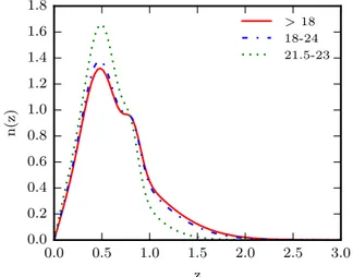
dispersion ofσ=0.277 (see Heymans et al.2012for details). Fig.1shows the source redshift distributionsn(z) for the three different magnitude cuts we have examined. Note that the lensing signal is most sensitive in the redshift range approximately half way between the sources and the observer. RCSLenS is shallower than the CFHTLenS (see the analysis in van Waerbeke et al.2013) but, as we demonstrate later, the larger area coverage of RCSLenS (more than) compensates for the lower number density of the source galaxies, in terms of the measurement of the cross-correlation with the tSZ signal.
Figure 1. Redshift distribution,n(z), of the RCSLenS sources for different
r-magnitude cuts. We work with the magr>18 cut (which includes all the
objects in the survey).
For our analysis we use the shear data and the reconstructed projected mass maps (convergence maps) from RCSLenS. For the tSZ–tangential shear cross-correlation (y–γt), we work at the
cat-alogue level where each pixel in theymap is correlated with the average tangential shear from the corresponding shear data in an annular bin around that point, as described in Section 3.1. To con-struct the convergence maps, we follow the method described in van Waerbeke et al. (2013). In Appendix A we study the impact of map smoothing on the SNR we determine for they–κcross-correlation analysis. We demonstrate that the best SNR is obtained when the maps are smoothed with a kernel that roughly matches the beam scale of the correspondingymaps fromPlancksurvey [full width at half-maximum (FWHM)=10 arcmin].
The noise properties of the constructed maps are studied in detail in Appendix B.
2.2.2 PlancktSZ y maps
For the cross-correlation with the tSZ signal, we use the full sky maps provided in thePlanck2015 public data release (Planck Col-laboration XXII2016). We use themilcamap that has been con-structed from multiple frequency channels of the survey. Since we are using the public data from thePlanckcollaboration, there is no significant processing involved. Our map preparation procedure is limited to masking the map and cutting the patches matching the RCSLenS footprint.
Note that in performing the cross-correlations we are limited by the footprint area of the lensing surveys. In the case of RCSLenS, we have 14 separate compact patches with different sizes. In con-trast, the tSZymaps are full-sky (except for masked regions). We therefore have the flexibility to cut out larger regions around the RCSLenS fields, in order to provide a larger cross-correlation area that helps suppress the statistical noise, leading to an improvement in the SNR. We cut outymaps so that there is complete overlap with RCSLenS up to the largest angular separation in our cross-correlation measurements.
Templates have also been released by thePlanckcollaboration to remove various contaminating sources. We use their templates to mask galactic emission and point sources, which amounts to remov-ing∼40 per cent of the sky. We have compared our cross-correlation measurements with and without the templates and checked that our
signal is robust. We have also separately checked that the masking of point sources has a negligible impact on our cross-correlation signal (see Appendix A). These sources of contamination do not bias our cross-correlation signal and contribute only to the noise level.
In addition to using the tSZ map from thePlanckcollaboration, we have also tested our cross-correlation results with the maps made independently following the procedure described in van Waerbeke et al. (2014), where several full-skyymaps were constructed from the second release ofPlanckCMB band maps. To construct the maps, a linear combination of the four High Frequency Instru-ment (HFI) band maps (100, 143, 217 and 353 GHz) was used and smoothed with a Gaussian beam profile withθSZ, FWHM= 10
ar-cmin. To combine the band maps, band coefficients were chosen such that the primary CMB signal is removed, and the dust emis-sion with a spectral indexβdis nulled. A range of models with
differentβdvalues were employed to construct a set ofymaps that
were used as diagnostics of residual contamination. The resulting cross-correlation measurements vary by roughly 10 per cent be-tween the differentymaps, but are consistent within the errors with the measurements from the publicPlanckmap.
2.3 Theoretical models
We compare our measurements with theoretical predictions based on the halo model and from full cosmological hydrodynamical sim-ulations. Below we describe the important aspects of these models.
2.3.1 Halo model
We use the halo model description for the tSZ–lensing cross-correlation developed in Ma et al. (2015). In the framework of the halo model, they–κcross-correlation power spectrum is
Cy–κ=C y–κ,1h
+C
y–κ,2h
, (13)
where the 1-halo and 2-halo terms are defined as
Cy–κ,1h=
zmax 0 dz dV dzd Mmax Mmin dM dn
dMy(M, z)κ(M, z),
Cy–κ,2h=
zmax
0
dz dV dzd P
lin
m(k=/χ , z)
×
Mmax
Mmin
dM dn
dMb(M, z)κ(M, z)
×
Mmax
Mmin
dM dn
dMb(M, z)y(M, z)
. (14)
In the above equations Plin
m(k, z) is the 3D linear matter power
spectrum at redshiftz, κ(M, z) is the Fourier transform of the convergence profile of a single halo of massMat redshiftzwith the Navarro–Frenk–White (NFW) profile,
κ= Wκ(z)
χ2(z)
1 ¯ ρm
rvir
0
dr(4πr2)sin(r/χ)
r/χ ρ(r;M, z), (15)
andy(M,z) is the Fourier transform of the projected gas pressure profile of a single halo,
y= 4πrs
2 s
σT
mec2 ∞
0
dx x2sin(x/s)
x/s
Pe(x;M, z). (16)
Herex≡a(z)r/rsands=aχ /rs, wherersis the scale radius of the
3D pressure profile, andPeis the 3D electron pressure. The ratio
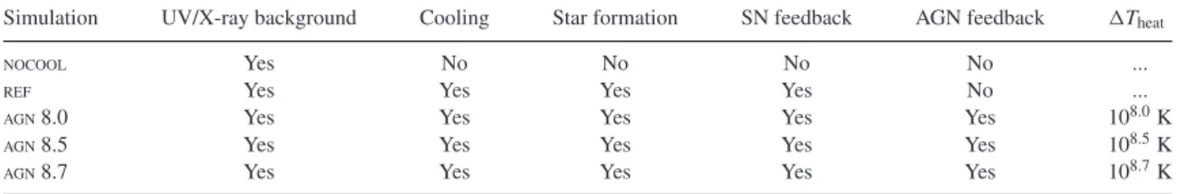
Table 1. Subgrid physics of the baryon feedback models in the cosmo-OWLS runs. Each model has been run adopting both theWMAP
7-yr andPlanckcosmologies.
Simulation UV/X-ray background Cooling Star formation SN feedback AGN feedback Theat
NOCOOL Yes No No No No ...
REF Yes Yes Yes Yes No ...
AGN8.0 Yes Yes Yes Yes Yes 108.0K
AGN8.5 Yes Yes Yes Yes Yes 108.5K
AGN8.7 Yes Yes Yes Yes Yes 108.7K
For the electron pressure of the gas in haloes, we adopt the so-called ‘universal pressure profile’ (UPP; Arnaud et al.2010):
P(x≡r/R500)=1.65×10−3E(z)
8 3
M500
3×10¹⁴h−1 70 M
2 3+0.12
×P(x)h270(keV cm− 3
), (17)
whereP(x) is the generalized NFW model (Nagai, Kravtsov & Vikhlinin2007):
P(x)= P0
(c500x)γ[1+(c500x)α](β−γ)/α
. (18)
We use the best-fitting parameter values from Planck Collaboration V (2013): {P0, c500, α, β, γ}= {6.41, 1.81, 1.33, 4.13, 0.31}. To compute the configuration-space correlation functions, we use equations (7) and (11) forξy–κandξy–γt, respectively. We present
the halo model predictions for two sets of cosmological param-eters: the maximum likelihoodPlanck 2013 cosmology (Planck Collaboration XVI2014) and the maximum likelihoodWMAP7-yr cosmology (Komatsu et al.2011) with { m, b, ,σ8,ns, h}
={0.3175, 0.0490, 0.6825, 0.834, 0.9624, 0.6711}and {0.272, 0.0455, 0.728, 0.81, 0.967, 0.704}, respectively.
There are several factors that have an impact on these predictions: the choice of the gas pressure profile, the adopted cosmological parameters and then(z) distribution of sources in the lensing sur-vey. In addition, the hydrostatic mass bias parameter,b(defined as
Mobs,500=(1−b)Mtrue,500), alters the relation between the adopted pressure profile and the true halo mass. Typically, it has been sug-gested that 1−b≈0.8. Note that the impact of the hydrostatic mass bias in real groups and clusters will be absorbed into our amplitude fitting parameterAtSZ(defined in equation 24).
2.4 The cosmo-OWLS hydrodynamical simulations
We also compare our measurements to predictions from the cosmo-OWLS suite of hydrodynamical simulations. In Hojjati et al. (2015) we compared these simulations to measurements using CFHTLenS data and we also demonstrated that high-resolution tSZ–lensing cross-correlations have the potential to simultaneously constrain cosmological parameters and baryon physics. Here we build on our previous work and employ the cosmo-OWLS simulations in the modelling of RCSLenS data.
The cosmo-OWLS suite is an extension of the OverWhelmingly Large Simulations (OWLS) project (Schaye et al.2010). The suite consists of box-periodic hydrodynamical simulations with volumes of (400h−1Mpc)3and 10243baryon and dark matter particles. The
initial conditions are based on either theWMAP7-yr orPlanck2013 cosmologies. We quantify the agreement of our measurements with the predictions from each cosmology in Section 5.
We use five different baryon models from the suite as summa-rized in Table1and described in detail in Le Brun et al. (2014) and McCarthy et al. (2014) and references therein. NOCOOL is a
standard non-radiative (‘adiabatic’) model.REFis the OWLS
refer-ence model and includes subgrid prescriptions for star formation (Schaye & Dalla Vecchia2008), metal-dependent radiative cooling (Wiersma, Schaye & Smith 2009a), stellar evolution, mass loss, chemical enrichment (Wiersma et al.2009b) and a kinetic super-nova feedback prescription (Dalla Vecchia & Schaye2008). The
AGNmodels are built on theREFmodel and additionally include a prescription for black hole growth and feedback from AGN (Booth & Schaye2009). The threeAGNmodels differ only in their choice of the key parameter of the AGN feedback modelTheat, which is the temperature by which neighbouring gas is raised due to feedback. Increasing the value ofTheat results in more energetic feedback events, and also leads to more bursty feedback, since the black holes must accrete more matter in order to heat neighbouring gas to a higher adiabat.
Following McCarthy et al. (2014), we produce light cones of the simulations by stacking randomly rotated and translated simulation snapshots (redshift slices) along the LoS back toz=3. Note that we use 15 snapshots at fixed redshift intervals betweenz=0 andz=3 in the construction of the light cones. This ensures a good comoving distance resolution, which is required to capture the evolution of the halo mass function and the tSZ signal. The light cones are used to produce 5◦×5◦maps of they, shear (γ1, γ2) and convergence
(κ) fields. We construct 10 different light cone realizations for each feedback model and for the two background cosmologies. Note that in the production of the lensing maps we adopt the source redshift distribution,n(z), from the RCSLenS survey to produce a consistent comparison with the observations.
From our previous comparisons to the cross-correlation of CFHTLenS weak lensing data with the initial publicPlanckdata in Hojjati et al. (2015), we found that the data mildly preferred a
WMAP7-yr cosmology to the Planck2013 cosmology. We will revisit this in Section 5 in the context of the new RCSLenS data.
3 O B S E RV E D C R O S S - C O R R E L AT I O N
Below we describe our cross-correlation measurements between tSZyand galaxy lensing quantities using the configuration-space and Fourier-space estimators described in Section 2.1.1.
3.1 Configuration-space analysis
We perform the cross-correlations on the 14 RCSLenS fields. The measurements from the fields converge around the mean values at each bin of angular separation with a scatter that is due to statistical noise and sampling variance. To combine the fields, we take the weighted mean of the field measurements, where the weights are determined by the totallensfit weight (see Miller et al.2013for technical definitions).
Figure 2. Cross-correlation measurements ofy–κ(left) andy–γt(right) from RCSLenS. The larger (smaller) error bars represent uncertainties after (before)
including our estimate of the sampling variance contribution (see Section 4). Halo model predictions using UPP withWMAP7-yr andPlanckcosmologies are also overplotted for comparison.
increase the cross-correlation area. For RCSLenS, we extend our measurements to an angular separation of 3◦, and hence include 4◦ wide bands around the RCSLenS fields.
We compute our configuration-space estimators as described be-low. For y–γt, we work at the catalogue level and compute the
two-point correlation function as
ξy–γt(ϑ)=
ijy ieij
t wjij(ϑ)
ijwjij(ϑ) 1
1+K(ϑ), (19)
whereyiis the value of pixeliof the tSZ map,eij
t is the tangential
ellipticity of galaxyjin the catalogue with respect to pixeliand wjis thelensfit weight. The (1+K(ϑ))−1factor accounts for the
multiplicative calibration correction (see Hildebrandt et al.2016for details):
1 1+K(ϑ) =
ijwjij(ϑ)
ijwj(1+mj)ij(ϑ)
. (20)
Finally,ij(ϑ) is imposes our binning scheme and is 1 if the angular
separation is inside the bin centred atϑand 0 otherwise.
For they–κ cross-correlation, we use the corresponding mass maps for each field and compute the correlation function as
ξy–κ(ϑ)=
ijy iκj
ij(ϑ)
ijij(ϑ)
, (21)
whereκjis the convergence value at pixeljand includes the
neces-sary weighting,wj.
Fig.2presents our configuration-space measurement of the RC-SLenS cross-correlation withPlancktSZ. Our measurements are performed within eight bins of angular separation, square-root-spaced between 1 and 180 arcmin. That is, the bins are uniformly spaced between√1 and√180. The filled circle data points show the
y–κ(left) andy–γt(right) cross-correlations. To guide the eye, the
solid red curves and dashed green curves represent the predictions of the halo model forWMAP7-yr andPlanck2013 cosmologies, respectively.
3.2 Fourier-space measurements
In the Fourier-space analysis, we work with the convergence and tSZ maps. As detailed in Harnois-D´eraps et al. (2016), it is
important to account for a number of numerical and observational effects when performing the Fourier-space analysis. These effects include data binning, map smoothing, masking, zero-padding and apodization. Failing to take such effects into account will bias the cross-correlation measurements significantly.
Here we adopt the forward modelling approach described in Harnois-D´eraps et al. (2016), where theoretical predictions are turned into a ‘pseudo-C’, as summarized below. First, we obtain the theoreticalC predictions from equations (13) and (14) as de-scribed in Section 2.3.1. We then multiply the predictions by a Gaussian smoothing kernel that matches the Gaussian filter used in constructing theκmaps in the mass map making process, and another smoothing kernel that accounts for the beam effect of the
Plancksatellite.
Next we include the effects of observational masks on our power spectra that break down into three components (see Harnois-D´eraps et al.2016for details): (i) an overall downward shift of power due to the masked pixels that can be corrected for with a rescaling by the number of masked pixels; (ii) an optional apodization scheme that we apply to the masks to smooth the sharp features introduced in the power spectrum of the masked map that enhance the high-power spectrum measurements and (iii) a mode mixing matrix that propagates the effect of mode coupling due to the observational window.
As shown in Harnois-D´eraps et al. (2016), steps (ii) and (iii) are not always necessary in the context of cross-correlation when the masks from both maps do not strongly correlate with the data. We have checked that this is indeed the case by measuring the cross-correlation signal from the cosmo-OWLS simulations with and without applying different sections of the RCSLenS masks, with and without apodization and observed that changes in the results were minor. We therefore choose to remove the steps (ii) and (iii) from the analysis pipeline. As the last step in our forward modelling, we re-bin the modelled pseudo-C so that it matches the binning scheme of the data. Note that these steps have to be calculated separately for each individual field due to their distinct masks.
Fig.3shows our Fourier-space measurement for they–κ cross-correlation, where halo model predictions for theWMAP7-yr and
Figure 3. Similar to Fig.2but for Fourier-space estimator,Cy–κ.
overall. Namely, the data points provide a better match toWMAP
7-yr cosmology prediction on small physical scales (largemodes) and tend to move towards thePlanckprediction on large physical scales (smallmodes). A more detailed comparison is non-trivial as different scales (modes) are mixed in the configuration-space measurements.
The details of error estimation and the significance of the detec-tion are described in Secdetec-tion 4.
4 E S T I M AT I O N O F C OVA R I A N C E M AT R I C E S A N D S I G N I F I C A N C E O F D E T E C T I O N
In this section, we describe the procedure for constructing the co-variance matrix and the statistical analysis that we perform to es-timate the significance of our measurements. We have investigated several methods for estimating the covariance matrix for the type of cross-correlations performed in this paper.
4.1 Configuration-space covariance
To estimate the covariance matrix we follow the method of van Waerbeke et al. (2013). We first produce 300 random shear cata-logues from each of the RCSLenS fields. We create these catacata-logues by randomly rotating the individual galaxies. This procedure will destroy the underlying lensing signal and create catalogues with pure statistical lensing noise. We then construct they–γtcovariance
matrix,Cy–γt, by cross-correlating the randomized shear maps for
each field with theymap.
To construct they–κcovariance matrix, we perform our standard mass reconstruction procedure on each of the 300 random shear cat-alogues to get a set of convergence noise maps. We then compute the covariance matrix by cross-correlating theymaps with these random convergence maps. We follow the same procedure of map making (masking, smoothing, etc.) in the measurements from ran-dom maps as we did for the actual measurement. This ensures that our error estimation is representative of the underlying covariance matrix.
Note that we also need to ‘debias’ the inverse covariance matrix by a debiasing factor as described in Hartlap, Simon & Schneider (2007):
α=(n−p−2)/(n−1), (22)
wherepis the number of data bins andnis the number of random maps used in the covariance estimation.2
The correlation coefficients are shown in Fig.4fory–κ (left) andy–γt(right). As a characteristic of configuration space, there
is a high level of correlation between pairs of data points within each estimator. This is more pronounced fory–κ since the mass map construction is a non-local operation, and also that the maps are smoothed that creates correlation by definition. Having a lower level of bin-to-bin correlations is another reason why one might want to work with tangential shear measurements rather than mass maps in such cross-correlation studies.
4.2 Fourier-space covariance
For the covariance matrix estimation in Fourier space, we follow a similar procedure as in configuration space. We first Fourier trans-form the random convergence maps, and then follow the same anal-ysis for the measurements (see Section 3). The resulting cross-correlation measurements create a large sample that can be used to construct the covariance matrix. Similar to the configuration-space analysis, we also debias the computed covariance matrix.
Fig.4, right-hand panel, shows the cross-correlation coefficients for thebins (Note that we chose to work with five linearly spaced bins between=100 and=2000.) As expected, there is not much bin-to-bin correlation and the off-diagonal elements are small.
4.3 Estimating the contribution from the sampling variance
Constructing the covariance matrix as described above includes the statistical noise contribution only. There is, however, a considerable scatter in the cross-correlation signal between the individual fields. A comparison of the observed scatter to that among different LoS of the (noise-free) simulations shows that the sampling variance contribution is non-negligible. We therefore need to include the contribution to the covariance matrix from sampling variance.
We are not able, however, to estimate a reliable covariance matrix that includes sampling variance since the number of samples we have access to is very limited and the resulting covariance matrix will be noisy and non-invertible. We only have a small number of fields from the lensing surveys (14 fields from RCSLenS is not nearly enough) and the same is true for the number of LoS maps from hydrodynamical simulations (10 LoS). Instead, we can estimate the sampling variance contribution by quantifying by how much we need to ‘inflate’ our errors to account for the impact of sampling variance.
Note that the scatter in the cross-correlation signal from the indi-vidual fields is due to both statistical noise and sampling variance. We compare the scatter (or variance) in each angular bin to that of the diagonal elements of the reconstructed covariance matrix that we obtained from the previous section (which quantifies the statis-tical uncertainty alone). We estimate the scaling factor by which we should inflate the computed covariance matrix to match the observed scatter.
The ratio between the variance between the fields and the sta-tistical covariance is scale independent for the tangential shear but shows some scale dependence for the other two estimators. We therefore wish to find a simple description of the ratioriat some
2In principle we should also implement the treatment of Sellentin & Heavens
Figure 4. Cross-correlation coefficient matrix of the angular bins for the configuration-spacey–κ(left) andy–γt(middle), and the Fourier-spacey–κ(right)
estimators. Angular bins are more correlated for they–κestimator compared toy–γtor the Fourier-space estimator.
Figure 5. Ratios of the variance between the 14 RCSLenS fields and the variance estimated from random shear maps, as described in Section 4. The best-fitting linear model for the ratios is shown in green.
scaleibetween the field variance and statistical covariance, such that the statistical covarianceCstatcan be rescaled as
Cij =Cstatij
√
rirj. (23)
We model the ratiorias a liner function of the scale. The model is then fit to the observer ratios between the field variances and statistical covariance. The errors on the observed ratios are estimated by taking 1000 bootstrap resamplings of the 14 RCSLenS fields and calculating the ratio from the variance of those resampled fields. The errors are highly correlated themselves but the error covariance is not invertible for the same reason the data covariance of the 14 fields is not invertible; the number of independent fields is too small. The observed ratios and the best-fitting modelsriare shown in Fig.5. We use these best-fitting models to rescale the statistical covariance according to equation (23) to obtained an estimate of the full covariance.
4.4 χ2analysis and significance of detection
We quantify the significance of our measurements using the SNR estimator as described below. We assume that the RCSLenS fields are sufficiently separated such that they can be treated as indepen-dent, ignoring field-to-field covariance.
First, we introduce the cross-correlation bias factor,AtSZ, through
V=ξ˜−AtSZξ .ˆ (24)
AtSZquantifies the difference in amplitude between the measured ( ˜ξ) and predicted ( ˆξ) cross-correlation function. The prediction can be from either the halo model or from hydrodynamical simulations. UsingV, we define theχ2as
χ2=VC−1VT, (25)
Table 2. A summary of theχnull2 values before and after including the sampling variance contribution according to the adjustment procedure of Section 4.3. There are eight angular bins, or degrees of freedom (DoF), at which the individual estimators are computed. Combining the estimators increases the DoF accordingly.
Estimator DoF χ2
null, stat. err. only χnull2 , adjusted
ξy–κ 8 193.5 56.2
ξy–γt 8 307.4 71.6
Combined 16 328.7 124.2
Cy–κ 5 156.4 64.9
whereCis the covariance matrix. We defineχ2
nullby settingAtSZ=0. In addition,χ 2
minis found by
minimizing equation (25) with respect toAtSZ:
χnull2 :AtSZ=0, (26)
χmin2 :AtSZ,min. (27)
In other words,χ2
min quantifies the goodness of fit between the
measurements and our model prediction after marginalizing over
AtSZ.
Table2summarizes theχ2
nullvalues from the measurements
be-fore and after including the sampling variance contribution. The values are quoted for individual estimators and when they are com-bined. Theχ2
nullis always higher fory–γtestimator, demonstrating
that it is a better estimator for our cross-correlation analysis. It also improves when we combine the estimators but we should consider thatχ2
nullincreases at the expense of adding extra degrees of freedom
Table 3. A summary of the statistical analysis of the cross-correlation measurements. For the configuration-space estimators, the results are shown for each estimator independently and when they are combined. SNR quantifies the significance of detection after a fit to model predictions (halo model). SNR values are shown before (SNR, stat. err. only) and after (SNR, adjusted) adjustment for sampling variance uncertainties according to the description of Section 4.3, whileAtSZvalues are quoted after the adjustment. ThePlanckcosmology predicts higher amplitude
thanWMAP7-yr cosmology so that overall, theWMAP7-yr cosmology predictions are in better agreement with the measurements.
Estimator SNR, stat. err. only SNR, adjusted Atsz,WMAP7-yr Atsz,Planck
ξy–κ 13.3 7.1 1.18±0.17 0.64±0.09
ξy–γt 16.8 8.1 1.27±0.16 0.68±0.08
Combined 17.1 10.6 1.23±0.12 0.66±0.06
Cy–κ 11.6 7.5 1.07±0.14 0.60±0.08
due to the correlation between the two estimators so thatχ2 nulldoes
not increase by a factor of 2.
Finally, we define the SNR as follows. We wish to quantify how strongly we can reject the null hypothesisH0, that no correlation exists between lensing and tSZ, in favour of the alternative hypoth-esisH1, that the cross-correlation is well described by our fiducial model up to a scaling by the cross-correlation biasAtSZ. To this end, we employ a likelihood ratio method. The devianceDis given by the logarithm of the likelihood ratio betweenH0andH1:
D= −2 logL(d|H0) L(d|H1)
. (28)
For Gaussian likelihoods, the deviance can then be written as D=χnull2 −χ
2
min. (29)
IfH1can be characterized by a single, linear parameter,Dis dis-tributed asχ2with one degree of freedom (Williams2001). The
significance in units of standard deviationsσof the rejection of the null hypothesis, i.e. the significance of detection, is therefore given by
SNR= χ2
null−χmin2 . (30)
Table3summarizes the significance analysis of our measure-ments. We show the SNR and best-fitting amplitudeAtSZ, for the theoretical halo model predictions withWMAP7-yr and Planck
cosmologies. The results are presented for each estimator indepen-dently and for their combination. Note that all the values in Table3 are adjusted to account for the sampling variance, as described in Section 4.3. To estimate the combined covariance matrix, we place the covariance for individual estimators as block diagonal elements of combined matrix and compute the off-diagonal blocks (the co-variance between the two estimators).
The predictions from WMAP 7-yr cosmology are relatively favoured in our analysis, which is consistent with the results of pre-vious studies (e.g. McCarthy et al.2014; Hojjati et al.2015). We, however, find similar SNR values from both cosmologies because the effect of the different cosmologies on the halo model prediction can be largely accounted for by an overall rescaling (AtSZ). After rescaling, the remaining minor differences are due to the shape of the cross-correlation signal so that the SNR depends only weakly on the cosmology.
We obtain a 13.3σ and 16.8σ from y–κ and y–γt estimators,
respectively, when we only consider the statistical noise in the co-variance matrix (before the adjustment prescription of Section 4.3).3
3Note that we are quoting the detection levels from a statistical noise-only
covariance matrix so that we can compare to the previous literature, including
The 13.3σsignificance fromy–κestimator should be compared to the ∼6σ detection from the same estimator in van Waerbeke et al. (2014) where CFHTLenS data are used instead. As expected, RCSLenS yields an improvement in the SNR andy–γtimproves
it further. Including sampling variance in the covariance matrix decreases the detection significance from RCSLenS data to 7.1σ and 8.1σfor they–κandy–γtestimators, respectively.
We perform a similar analysis in Fourier space where the data vector is given by the pseudo-Cs and the results are included in Table3. The SNR values are in agreement with the configurations-space analysis.4We see a similar trend as in the configuration-space
analysis in that there is a better agreement with theWMAP7-yr halo model predictions (AtSZis closer to 1) while thePlanckcosmology predicts a high amplitude.
Table3summarizes the predictions from the halo model frame-work with a fixed pressure profile for gas (UPP). In Section 5, we revisit this by comparing to predictions from hydrodynamical sim-ulations where haloes with different mass and at different redshifts have a variety of gas pressure profiles. We show that we find better agreement with models where AGN feedback is present in haloes.
4.5 Impact of maximum angular separation
The two configuration-space estimators we use probe different dy-namical scales by definition. This means that as we include cross-correlations at larger angular scales, information is captured at a different rate by the two estimators. For a survey with limited sky coverage, combining the two estimators will therefore improve the SNR of the measurements. In the following, we quantify this im-provement of the SNR.
In Fig.6, we plot the SNR values as a function of the maximum angular separation for both estimators. In addition, we also include the same quantities when debiased using equation (22) to highlight the effect of increasing DoF on the debiasing factor. Each angular bin is 10 arcmin wide and adding more bins means including cross-correlation at larger angular scales.
We observe that they–κmeasurement starts off with a higher SNR relative toy–γtat small angular separations. The SNR iny–
κ levels off very quickly with little information added above 1◦ separation. The shallow SNR slope of they–κcurve is partly due
the results of van Waerbeke et al. (2014), where a similar approach is taken in the construction of the covariance matrix (i.e. only statistical noise is considered).
4Note that the Fourier-space analysis is performed by pipeline 3 in
Figure 6. The SNR as a function of the maximum angular separation for the two configuration-space estimators, with and without debiasing (as de-scribed in Section 4.1). The slope of the lines is different for the two esti-mators due to the different information they capture as a function of angular separation. Fory–κ, most of the signal is in the first few bins making it a better candidate at small scales, whiley–γthas a larger slope and catches
up quickly. Eventually, the two estimators approach a plateau where they contain the same amount of cross-correlation information. Note that the plots show the SNR before the ‘adjustment’ procedure of Section 4.3.
to the Gaussian smoothing kernel that is used in reconstructing the mass maps which spreads the signal within the width of the kernel. They–γtcross-correlation, on the other hand, has a higher
rate of gain in SNR and catches up with the convergence rapidly. Eventually, the two estimators approach a plateau as the cross-correlation signals drop to zero. At that point, both contain the same amount of cross-correlation information.
Note that we limit ourselves to a maximum angular separation of 3◦in the RCSLenS measurements since the measurement is very noisy beyond that. Fig.6indicates that the two estimators might not have converged to the limit where the information is saturated (a plateau in the SNR curve). Since each estimator captures different information up to 3◦, combining them improves the measurement significance (see Table3). With surveys like the Kilo-Degree Sur-veys (KiDS; de Jong et al.2013), the Dark Energy Survey (DES; Abbott et al. 2016) and the Hyper Suprime-Cam Survey (HSC; Miyazaki et al.2012), where the coverage area is larger, we will be able to go to larger angular separations where the information from our estimators is saturated. The signal at such large scales is primar-ily dependent on cosmology and quite independent of the details of the astrophysical processes inside haloes (see Hojjati et al.2015 for more details). This could, in principle, provide a new probe of cosmology based on the cross-correlation of baryons and lensing on distinct scales and redshifts.
5 I M P L I C AT I O N S F O R C O S M O L O G Y A N D A S T R O P H Y S I C S
In Section 3, we compared our measurements to predictions from the theoretical halo model. The halo model approach, however, has limitations for the type of cross-correlation we are considering. For example, in our analysis we cross-correlate every source in the sky that produces a tSZ signal with every source that produces a lensing signal. A fundamental assumption of the halo model, however, is that all the mass in the Universe is in spherical haloes, which is not an accurate description of the large-scale structure in
Figure 7. Comparisons of our cross-correlation measurement from RC-SLenS to predictions from hydrodynamical simulations. The larger (smaller) error bars represent uncertainties after (before) including our estimate of the sampling variance contribution (see Section 4). Different baryon feedback models withWMAP7-yr cosmology are shown fory–γtestimator (we are
not showing the plots fory–κas they are very similar). Baryon feedback has an impact on the cross-correlation signal at small scales.
the Universe. There are other structures such as filaments, walls or free flowing diffuse gas in the Universe, so that matching them with spherical haloes could lead to biased inference of results (see Hojjati et al.2015). Another shortcoming is that our halo model analysis considers a fixed pressure profile for diffuse gas, while it has been demonstrated in various studies that the UPP does not necessarily describe the gas around low-mass haloes particularly well (e.g. Battaglia et al.2012; Le Brun, McCarthy & Melin2015). Here we employ the cosmo-OWLS suite of cosmological hy-drodynamical simulations (see Section 2.4) that includes various simulations with different baryonic feedback models. The cosmo-OWLS suite provides a wide range of tSZ and lensing (convergence and shear) maps allowing us to study the impact of baryons on the cross-correlation signal. We follow the same steps as we did with the real data to extract the cross-correlation signal from the simulated maps.
Fig. 7 compares our measured configuration-space cross-correlation signal to those from simulations with different feedback models. The plots are for the five baryon models using theWMAP
7-yr cosmology, and theAGN8.0 model using thePlanckcosmology
is also plotted for comparison. Note that baryon models make the largest difference at small scales due to mechanisms that change the density and temperature of the gas inside clusters. For the (non-physical)NOCOOLmodel, the gas can reach very high densities near the centre of dark matter haloes and is very hot since there is no cooling mechanism in place. This leads to a high tSZ and hence a high cross-correlation signal. After including the main baryonic processes in the simulation (e.g. radiative cooling, star formation and SN winds), we see that the signal drops on small scales. Adding AGN feedback warms up the gas but also expels it to larger dis-tances from the centre of haloes. This explains why we see a lower signal at small scales but a higher signal at intermediate scales for theAGN8.7 model. Note that the scatter of the LoS signal varies for different models due to the details of the baryon processes so that, for example, theAGN8.7 model creates a larger sampling variance.
Figure 8. Same as Fig.7but for the Fourier-space estimator,Cy–κ.
produces a higher signal at all scales and for all models. This is mainly due to the larger values of b, mand particularlyσ8, in
thePlanck2013 cosmology compared to that of theWMAP7-yr cosmology.
We summarize in Table4ourχ2 analysis for feedback model
predictions relative to our measurements. We find that the data prefer aWMAP7-yr cosmology to thePlanck2013 cosmologyfor all of the baryon feedback models. This is worth stressing, given the very large differences between the models in terms of the hot gas properties that they predict (Le Brun et al.2014), which bracket all of the main observed scaling relations of groups and clusters. The best-fitting models are underlined for both cosmologies.
Our measurements are limited by the relatively low resolution of thePlancktSZ maps. On small scales, our signal is diluted due to the convolution of the tSZ maps with thePlanckbeam (FWHM=10 ar-cmin) that makes it hard to discriminate the feedback models with our configuration-space measurements. This highlights that high-resolution tSZ measurements can be particularly useful to overcome this limitation and open up the opportunity to discriminate the feed-back models from tSZ–lensing cross-correlations.
The feedback models could be better discriminated in Fourier space through their power spectra. We therefore repeat our mea-surements on the simulation in the Fourier space. We apply the same procedure described in Section 3.2 to the simulated maps. Fig.8compares our power spectrum measurements to simulation predictions, and we have summarized theχ2analysis in Table4.
Our Fourier-space analysis follows a similar trend as the configuration-space analysis. Namely, there is a general overpre-diction of the amplitude that is worse for thePlanckcosmology. For the best-fittingWMAP7-yr models the fitted amplitude is con-sistent with 1. Our estimator prefers theAGN8.7 model in all cases
with aPlanckcosmology that is different than configuration-space estimator where theAGN8.5 was preferred.5There are a few reasons
for these minor differences. For example, the binning schemes are different and give different weights to bins of angular separation. Furthermore, the Fourier-based result can change by small amounts depending on precisely which pipeline from Harnois-D´eraps et al. (2016) is adopted.
5We tested that if large-scale correlations (ϑ >100 arcmin), where
uncer-tainties are large, are removed from the analysis, theAGN8.7 model is also
equally preferred by the configuration-space estimators.
When we fit the amplitudeAtSZto obtain theχ2
minor SNR values,
we are in fact factoring out the scaling of the model prediction and are left with the prediction of the shape of the cross-correlation signal. The shape depends on both the cosmological parameters (weakly) and details of the baryon model so that the values in Ta-bles3and4are a measure of how well the model shape matches the measurement. By comparing theχ2
minvalues from the two
cos-mologies in Table4, the general conclusion of our analysis is that significant AGN feedback in baryon models is required to match the measurements well. Note, however, that while there are differ-ences in the amplitude (and shape) of the cross-correlation signal, the predictions from the two cosmology are not in tension with the measurements when one considers the current uncertainties in the values of the cosmological parameters (e.g.σ8).
6 S U M M A RY A N D D I S C U S S I O N
We have performed cross-correlations of the publicPlanck2015 tSZ map with the public weak lensing shear data from the RCSLenS. We have demonstrated that such cross-correlation measurements between two independent data sets are free from contamination by residual systematics in each data set, allowing us to make an initial assessment of the implications of the measured cross-correlations for cosmology and intracluster medium (ICM) physics.
Our cross-correlations are performed at the map level where ev-ery object is contributing to the signal. In other words, this is not a stacking analysis where measurements are done around identified haloes. Instead, we are probing all the structure in the Universe (haloes, filaments, etc.) and the associated baryon distribution in-cluding diffuse gas in the intergalactic medium.
We performed our analysis using two configuration-space esti-mators,ξy–γtandξy–κ, and a Fourier-space analysis withCy–κ
for
completeness. Configuration-space estimators have the advantage that they are less affected by the details of map making processes (masks, appodization, etc.) and the analysis is straightforward. We showed that the estimators probe different dynamical scales so that combining them can improve the SNR of the measurement.
Based only on the estimation of statistical uncertainties, the cross-correlation using RCSLenS data is detected with a significance of 13.3σ and 16.8σ from they–κandy–γtestimators, respectively.
Including the uncertainties due to the sampling variance reduces the detection to 7.1σ and 8.1σ, respectively. We demonstrated that RCSLenS data improve the SNR of the measurements significantly compared to previous studies where CFHTLenS data were used.
The Fourier-space analysis, while requiring significant process-ing to account for maskprocess-ing effects, is more useful for probprocess-ing the impact of physical effects at different scales. We work withCy–κ and test for consistency of the results with the configuration-space estimators. We reach similar conclusions for theCy–κ measure-ment as the configuration-space counterpart and the same level of significance of detection.
The high level of detection compared to similar measurements in van Waerbeke et al. (2014) is due to two main improvements: the larger sky coverage offered by RCSLenS has suppressed the statistical uncertainties of the measured signal, and the final tSZ map provided by thePlanckteam is also less noisy than that used in van Waerbeke et al. (2014).
Table 4. Summary ofχmin2 analysis of the cross-correlation measurements from hydrodynamical simulations. The error
on the best-fitting amplitudes is adjusted according to description of Section 4.3. The best-fitting models are underlined for both cosmologies. TheWMAP7-yr predictions fit data better for all baryon models. TheAGN8.5 model is preferred
by the configuration-space measurements while the Fourier-space measurements prefer theAGN8.7 model.
Model χ2
min,WMAP7-yr Atsz,WMAP7-yr χmin2 ,Planck Atsz,Planck
AGN8.0 5.3 1.00±0.12 5.4 0.68±0.08
AGN8.5 3.2 1.10±0.13 5.9 0.74±0.09
Config. space AGN8.7 8.6 1.01±0.13 8.3 0.72±0.09
NOCOOL 5.7 0.89±0.11 6.1 0.62±0.08
REF 5.7 1.06±0.13 5.8 0.74±0.09
AGN8.0 6.1 0.83±0.11 6.5 0.57±0.07
AGN8.5 3.3 1.01±0.13 4.0 0.68±0.09
Fourier space AGN8.7 1.4 1.20±0.15 1.7 0.83±0.10
NOCOOL 8.7 0.72±0.10 8.2 0.50±0.07
REF 7.2 0.86±0.11 7.2 0.61±0.08
the type of cross-correlation measurement we consider in this pa-per. Our error analysis includes contributions from both statistical uncertainty and sampling variance. The large sampling variance in the cross-correlation signal originates mainly from the tSZ maps due to the dependence of the tSZ signal on the halo mass, AGN feedback and other stochastic processes. We estimated its contribu-tion from field-to-field variance, but recognize that better estimacontribu-tion requires access to more data or more hydrodynamical simulations. Predictions from aWMAP7-yr best-fitting cosmology match the data better than those based on thePlanckcosmology, in agreement with previous studies (e.g. McCarthy et al.2014).
Finally, we employed the cosmo-OWLS hydrodynamical simu-lations (Le Brun et al.2014), using synthetic tSZ and weak lensing maps produced for a wide range of baryonic physics models in both theWMAP7-yr andPlanckcosmologies. In agreement with the findings of the halo model results, the comparison to the pre-dictions of the simulations yields a preference for theWMAP7-yr cosmology regardless of which feedback model is adopted. This is noteworthy, given the vast differences in the models in terms of their predictions for the ICM properties of groups and clusters (which bracket the observed hot gas properties of local groups and clusters; see Le Brun et al.2014). The detailed shape of the measured cross-correlations tends to prefer models that invoke significant feedback from AGN, consistent with what is found from the analysis of ob-served scaling relations, although there is still some degeneracy between the adopted cosmological parameters and the treatment of feedback physics. Future high-resolution CMB experiments com-bined with large sky area from a galaxy survey can in principle break the degeneracy between feedback models and place tighter constrains on the model parameters.
We highlighted the difficulties in estimating the covariance matrix for the type of cross-correlation measurement we consider in this paper. The large sampling variance in the cross-correlation signal, which originates mainly from the tSZ maps, requires access to more data or more hydrodynamical simulations to be accurately estimated. With the limited data we have, the covariance matrix that contained the contribution from sampling variance was noisy, making it impossible to perform a robust significance analysis of the measurements. This is an area where more work is required and we will pursue this in future work.
AC K N OW L E D G E M E N T S
We would like to thank the RCS2 team for conducting the survey, members of the RCSLenS team for producing the quality shear
data and the members of the OWLS team for their contributions to the development of the simulation code used here. We also thank Nicholas Battaglia and James C. Hill for useful discussions.
AH is supported by NSERC. TT is supported by the Swiss Na-tional Science Foundation (SNSF). JH-D acknowledges support from the European Commission under a Marie-Skłodwoska-Curie European Fellowship (EU project 656869). IGM is supported by a STFC Advanced Fellowship at Liverpool JMU. LvW and GH are supported by NSERC and the Canadian Institute for Advanced Research. AC acknowledges support from the European Research Council under the EC FP7 grant number 240185. TE is supported by the Deutsche Forschungsgemeinschaft in the framework of the TR33 ‘The Dark Universe’. CH acknowledges support from the European Research Council under grant number 647112. HH is supported by an Emmy Noether grant (No. HI 1495/2-1) of the Deutsche Forschungsgemeinschaft.
This paper made use of the RCSLenS ( http://www.cadc-ccda.hia-iha.nrc-cnrc.gc.ca/en/community/rcslens/query.html) and Planck
Legacy Archive (http://archives.esac.esa.int/pla) data.
R E F E R E N C E S
Abbott T. et al., 2016, Phys. Rev. D., 94, 022001
Arnaud M., Pratt G. W., Piffaretti R., B¨ohringer H., Croston J. H., Pointe-couteau E., 2010, A&A, 517, A92
Battaglia N., Bond J. R., Pfrommer C., Sievers J. L., 2012, ApJ, 758, 75 Battaglia N., Hill J. C., Murray N., 2015, ApJ, 812, 154
Ben´ıtez N., 2000, ApJ, 536, 571
Booth C. M., Schaye J., 2009, MNRAS, 398, 53 Coupon J. et al., 2015, MNRAS, 449, 1352
Dalla Vecchia C., Schaye J., 2008, MNRAS, 387, 1431 de Jong J. T. A. et al., 2013, The Messenger, 154, 44 Erben T. et al., 2013, MNRAS, 433, 2545
Gilbank D. G., Gladders M. D., Yee H. K. C., Hsieh B. C., 2011, AJ, 141, 94
Harnois-D´eraps J., van Waerbeke L., Viola M., Heymans C., 2015, MNRAS, 450, 1212
Harnois-D´eraps J. et al., 2016, MNRAS, 460, 434 Hartlap J., Simon P., Schneider P., 2007, A&A, 464, 399 Heymans C. et al., 2012, MNRAS, 427, 146
Hildebrandt H. et al., 2012, MNRAS, 421, 2355 Hildebrandt H. et al., 2016, MNRAS, 463, 635
Hill J. C., Spergel D. N., 2014, J. Cosmol. Astropart. Phys., 2, 030 Hojjati A., McCarthy I. G., Harnois-D´eraps J., Ma Y.-Z., Van Waerbeke L.,