Constrained parameter estimation with uncertain priors for Bayesian networks

Vol. 11 (2017) 4000–4032 ISSN: 1935-7524

DOI:10.1214/17-EJS1350

Constrained parameter estimation with

uncertain priors for Bayesian networks

∗

Ali Karimnezhad

Department of Statistics and Computer Science K. N. Toosi University of Technology, Tehran, Iran

e-mail:[email protected]

Peter J. F. Lucas

Institute for Computing and Information Sciences University of Nijmegen, Nijmegen, The Netherlands

e-mail:[email protected]

and

Ahmad Parsian†

School of Mathematics, Statistics and Computer Science University of Tehran, Tehran, Iran

e-mail:ahmad [email protected]

Abstract: In this paper we investigate the task of parameter learning of Bayesian networks and, in particular, we deal with the prior uncertainty of learning using a Bayesian framework. Parameter learning is explored in the context of Bayesian inference and we subsequently introduce Bayes, con-strained Bayes and robust Bayes parameter learning methods. Bayes and constrained Bayes estimates of parameters are obtained to meet the twin objective of simultaneous estimation and closeness between the histogram of the estimates and the posterior estimates of the parameter histogram. Treating the prior uncertainty, we consider some classes of prior distribu-tions and derive simultaneous Posterior Regret Gamma Minimax estimates of parameters. Evaluation of the merits of the various procedures was done using synthetic data and a real clinical dataset.

MSC 2010 subject classifications:Primary 62F15, 62C10; secondary 62F30, 62F35.

Keywords and phrases:Bayesian networks, constrained Bayes estima-tion, directed acyclic graph, posterior regret, robust Bayesian learning.

Received January 2017.

Contents

1 Introduction . . . 4001 ∗_{The authors are grateful to the Editor, an anonymous Associate Editor and an anonymous} referee for making valuable comments and suggestions on an earlier version of this article which led to substantial improvement.

†_{Ahmad Parsian’s research supported by a grant of the Research Council of the University} of Tehran.

4001

2 Preliminaries . . . 4002

2.1 Basic notions . . . 4002

2.2 Bayesian learning methods . . . 4004

3 Constrained Bayesian learning . . . 4005

4 Posterior regret Gamma minimax learning . . . 4007

5 Experiments . . . 4011

5.1 Synthetic data . . . 4011

5.2 Real clinical data . . . 4015

6 Final remarks . . . 4019

7 Conclusions and discussion . . . 4021

Appendix . . . 4022

References . . . 4029

1. Introduction

Bayesian networks (BNs) have become one of the most popular probabilistic models for representing joint probability distributions of a set of random vari-ables [7, 28, 33]. Learning BNs from data is normally split into two different, although related steps: (1) learning the structure of the network and (2) learning the parameters [8, 18]. Sometimes the network structure is designed using ex-pert knowledge. Once the structure of a network is obtained, parameter learning becomes possible.

Several methods are available to learn the structure of a BN (see [6,10,17,44] among others), and there are many good software implementations of many of these [e.g.30].

The focus of this paper is on the task of parameter learning only in BNs whose nodes represent discrete random variables. However, later in our final remarks, we refer to three common approaches of extending such BNs to BNs whose nodes are continuous random variables. Parameter learning has been studied also widely, giving rise to many different approaches. Most of the studies are based on the maximum likelihood (ML), the maximum a posteriori (MAP), or the posterior mean (PM) criterion. The ML estimation is a classical technique providing a parameter estimator by maximizing the joint probability density functions (pdfs), while the MAP and PM estimates, as Bayesian solutions, com-bine the information derived from the data witha priori knowledge concerning the parameter, see [4, 8,9,25,35] among others.

4002

notion of robustness used in this paper is different from the one explored by [34] in their description of the robust Bayes estimator, where they deal with missing data by means of probability intervals.

This paper is organized as follows: In Section2, we introduce some prelimi-naries. Section3is devoted to simultaneous Bayes and the idea of CB learning. In addition, explicit forms for parameter estimates are derived. In Section4, we introduce the idea of simultaneous posterior regret gamma minimax (SPRGM) learning in the presence of prior uncertainty and derive the corresponding es-timates. In Section 5, we carry out an experimental study and compare per-formance of the proposed estimators using synthetic data from a well-known example network. Further, we study the impact of the proposed methods using real clinical data and a real-world BN. Finally, we conclude with some final re-marks and a discussion. To keep readers in track, all the proofs along with some supplementary materials are provided in the Appendix.

2. Preliminaries

In this section we summarize the required basic material needed later. For more information see [8,18,24,25,31,40].

2.1. Basic notions

A BN consists of a set of variables (or nodes)V ={X1, . . . , Xd}and a subset of

directed linksE(also sometimes called edges or arcs) contained in the Cartesian product V ×V. We say the structure of a BN is known if the variables in the setV are connected to each other according to the links in E. Mathematically, the structure is called a directed graph. The directed graph is called acyclic, if it does not contain any directed cycle. We refer to such a directed acyclic graph (DAG) byG= (V, E). In the BNs context, a node is instantiated when its value is known through observing what it represents. We say we have a complete instantiation if all the nodes of a BN are simultaneously observed.

Suppose that for each j = 1, . . . , d, the variable Xj takes values in the set Xj = {x(1)j , . . . , x

(kj)

j }. The set of all possible outcomes for the experiment

may be denoted by X = X1× · · · × Xd. Hence, a sample of cases is given

byx= (x₍₁₎, . . . ,x_(n)), wherex(i)= (x(i,j11), . . . , x (jd)

i,d ) denotes thei-th complete

instantiation andx_(i)stands for the transpose ofx(i). For each variableXj,

de-note all possible instantiations of the parent set Λj by the set{λ(1)j , . . . , λ

(qj)

j }.

Thus, λ(_jl) implies that the parent configuration of variable Xj is in state λ(jl)

and there areqj possible configurations of Λj.

For a given graph structureG= (V, E), let

njilk=

1, if (x(_ji), λ_j(l)) is found inx(k)

4003

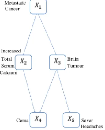
Fig 1_{. A 5-node DAG.}

where (x(_ji), λ(_jl)) is a configuration of the family (Xj,Λj). Letθ∈Θdenote the

set of parameters defined by

θjil=P

Xj=x(ji)|Λj =λ(jl)

, (2.2)

forl= 1, . . . , qj, i= 1, . . . , kj, j= 1, . . . , d, with

kj

i=1θjil= 1.

Using the decomposition of the probability distribution defined by the BN, the joint probability of a casex(k)may be written as

pX(k)|Θ(x(k)|θ, E)∝

d

j=1

qj

l=1

kj

i=1 θnjilk_jil .

For independent observations (x(1), . . . ,x(n)), the joint probability of the cases

is

pX|Θ(x|θ,G) ∝ n

k=1

d

j=1

qj

l=1

kj

i=1

θ_jilnjilk =

d

j=1

qj

l=1

kj

i=1 θ_jilnjil.,

wherenjil.=

n

k=1njilk, which is the likelihood function. One can observe that

the ML estimate ofθjilin Eq. (2.2) is given by

δ_jilM L= njil.

nj.l.

, (2.3)

where nj.l.=

kj i=1njil..

Observe that all parameters (θj1l, . . . , θjkjl) of a specific node Xj preserve

the inherent symmetry ofkj_i=1θjil= 1. We expect the corresponding estimates

(δj1l, . . . , δjkjl) preserve this symmetry and satisfy the constraint

kj

i=1δjil= 1.

This constraint is automatically achieved by the ML estimates in Eq. (2.3) and

kj

i=1δjilM L= 1.

Example 2.1. Consider the DAG depicted in Fig.1with five nodesX1, . . . , X5.

Suppose that all the nodes exceptX3are binary variables andX3 takes values 0,

4004

and the parent set ofX5 has three possible instantiationsλ(1)5 = 0,λ (2)

5 = 1and λ(3)₅ = 2. Suppose complete instantiations of 10 cases are available as below

x= ⎛ ⎜ ⎝ x(1) .. . x(10) ⎞ ⎟ ⎠= ⎛ ⎜ ⎜ ⎜ ⎜ ⎜ ⎜ ⎜ ⎜ ⎜ ⎜ ⎜ ⎜ ⎜ ⎜ ⎝

(0,0,1,0,1) (0,1,0,1,1) (1,1,1,0,1) (0,0,0,0,0) (1,0,2,0,1) (0,1,1,1,0) (0,1,2,1,1) (1,0,0,0,1) (0,0,0,0,0) (1,1,2,0,1)

⎞ ⎟ ⎟ ⎟ ⎟ ⎟ ⎟ ⎟ ⎟ ⎟ ⎟ ⎟ ⎟ ⎟ ⎟ ⎠

and we are interested in learning the parameters θ5l = (θ51l, θ52l), l = 1,2,3. The ML estimate of θ5l is given by δM L5l = (δ51M Ll , δ52M Ll ), where δ5M Lil =

n5il. n5.l.,

n5.l. =

2

i=1n5il.,i = 1,2, l = 1,2,3. So, the ML estimate of θ52 is given by

δM L

52 = (13, 2 3).

2.2. Bayesian learning methods

In Example 2.1, one might believe that the sequence (0,0,1,1,1) occurs in 80 percent of cases. If so, we could takea prioriknowledge into account, assuming that some prior knowledge in forms of a prior distribution is available.

To derive the Bayes estimate of θjil in Eq. (2.2), consider the conjugate

Dirichlet prior distribution Dir(αj1l, . . . , αjkjl), with pdf

π(θj1l, . . . , θjkjl) ∝ kj

i=1

θ_jilαjil−1, (2.4)

where 0 < θjil < 1,

kj

i=1θjil = 1 and αjil > 0. Given the data x = (x(1), . . . ,x(n)), it can be verified that (θj1l, . . . , θjkjl)|x∼Dir(nj1l.+αj1l, . . . , njkjl.+

αjkjl). Obviously the marginal posteriors have Beta distributions, i.e.,θjil|x∼

Beta(njil.+αjil, nj.l.+αj.l−njil.−αjil), whereαj.l =

kj i=1αjil.

It is easy to observe that the MAP and PM estimates ofθjil are

δM AP_jil = arg max

θjil π(θjil|X =x) =

njil.+αjil−1

nj.l.+αj.l−2

, (2.5)

δP M_jil =E[θjil|X =x] =

njil.+αjil

nj.l.+αj.l

. (2.6)

Example 2.2. (Example 2.1, cont.) To derive the MAP and PM estimates of θ5i2 = (θ512, θ522), consider the conjugate Dir(α512, α522)-prior with α512 = 1

andα522= 2. Then from (2.5) and (2.6),δ52M AP = (nn5125.2..++αα5125.2−−21,

n522.+α522−1

n5.2.+α5.2−2) =

(1₄,3₄)andδP M52 = (nn5125.2..++αα5125.2,

n522.+α522

n5.2.+α5.2) = ( 1 3,

4005

3. Constrained Bayesian learning

In the preceding section, assuming the squared error loss (SEL) function, we observed that if the only objective is simultaneous estimation of the BN param-etersθjl= (θj1l, . . . , θjkjl) withθjildefined in Eq. (2.2), the Bayes estimate is a

vector of posterior means, i.e.,δP M_jl = (δP M_j1l , . . . , δP M_jkjl) withδ_jilP M given by Eq. (2.6). In this section, following the idea of CB estimation of [29], we provide an adjusted version ofδP M

jil .

To avoid any unambiguity, we define the following key terms. Let δjl =

(δj1l, . . . , δjkjl) be a vector of arbitrary estimates of elements of θjl =

(θj1l, . . . , θjkjl) withθjil defined in Eq. (2.2). Define the sample mean and the

sample variance of ensemble of the estimates δjil by ¯δj.l = _kj1

kj

i=1δjil and

1

kj

kj i=1

δjil−¯δj.l

2

, respectively. Also, define the posterior expected sample mean (PESM) and the posterior expected sample variance (PESV) of ensemble of the parametersθjilby _kj1E kji=1θjil|X=x

and _kj1E kj_i=1θjil−θ¯j.l

2

|

X =x

with ¯θj.l =_kj1

kj

i=1θjil, respectively.

[29] suggested that problems with using posterior means as Bayes estimates might be dealt with by constructing a vector of CB estimators for which the sample mean and the sample variance of an ensemble of them are equal to the PESM and the PESV of an ensemble of parameters, respectively. Particularly, he proved that under normal likelihood with normal prior, the sampling variability of a collection of Bayes estimates is smaller than the posterior expectation of the corresponding population variability, see [16]. This property holds true in BNs, as provided in the following lemma. See the Appendix for a detailed verification of this inequality.

Lemma 3.1. LetδP M

jl = (δjP M1l , . . . , δjkjlP M)be a vector of PM’s ofθjl= (θj1l, . . . ,

θjkjl)withθjildefined in Eq. (2.2), w.r.t. some priorπ. Then, for a fixedj and

l, the sample variance of ensemble of the Bayes estimates in δP M

jl is smaller than the PESV of ensemble of parameters inθjl, i.e.,

1

kj kj

i=1

δP M_jil −δ¯P M_j.l 2< 1 kj

E

kj

i=1

θjil−θ¯j.l

2

|X =x

. (3.1)

where ¯δ_j.lP M= _kj1 kj_i=1δ_jilP M andθ¯j.l=_kj1

kj i=1θjil.

By the CB approach of [29], the empirical distribution function of CB esti-mates becomes close to the empirical distribution function of the corresponding unknown parameters. This way, the sampling variability of a collection of esti-mates is a better estimate of the underlying variability among the population parameters. For more details, see [11,13,14,15].

4006

Bayes estimators in problems such as disease mapping or environmental risk as-sessment. For example, in disease mapping it is supposed that there arekregions labeled with the indices 1,2, . . . , k. By this setting, [11] follows a hierarchical model for disease counts and estimate the true disease rates θi,i= 1,2, . . . , k.

For more information, see [11,16] and papers cited therein.

Now, consider the problem of estimatingθjildefined in (2.2) under the SEL

function for a fixedj andl. If interest lies in both simultaneous estimation and closeness between the distribution of estimates and the posterior distribution of the parameters, the idea of deriving CB estimation might be helpful. To make a motivation, it is of interest to compare our estimation problem with the disease mapping problem considered in [11]. In the latter problem, some levels were considered for the parameter of interest (the true disease ratesθi,i= 1,2, . . . , k)

and in our estimation problem, in a specific node and for a specific parent, the parameter of interest, i.e., θjil, has different levels when changingi in the set {1,2, . . . , kj}. Thus, CB estimation can be considered in order to meet the twin

objective of simultaneous estimation and closeness between the distribution of the estimates and the posterior distribution of the parameters.

Here, we consider the problem of obtaining CB estimates of θjil, subject to

the constraints considered by [29], and an additional constraint which is imposed due to the nature of parameter learning in BNs, i.e.,

(i)kj_i=1δjil=

kj

i=1E[θjil|X =x],

(ii) _kj1 kj_i=1(δjil−δ¯j.l)2=_kj1E kji=1(θjil−θ¯j.l)2|X=x

,

(iii) kj_i=1δjil= 1,

where ¯δj.l= _kj1

kj

i=1δjiland ¯θj.l= _kj1

kj i=1θjil.

It is interesting to note that sincekj_i=1θjil=

kj

i=1δP Mjil = 1, the constraint

(i) results in (iii). However, each one of the constraints (i) and (iii) plays its separate role and hence, we simultaneously consider both of these constraints for later use. The following theorem provides CB estimates of parameters in BNs. The main idea of this theorem comes from a proof that appeared in [29]. See the Appendix for a version of the proof compatible with the constraints considered in this paper.

Theorem 3.1. Let δP M

jl = (δjP M1l , . . . , δjkjP Ml) be a vector of PM’s of θjl w.r.t. some prior π. Then under the constraints (i)-(iii), the CB estimate of θjl is given byδCB

jl = (δCBj1l, . . . , δCBjkjl), whereδjilCB =ajlδjilP M+ (1−ajl)_kj1 and

ajl=

Sjl(x)−_kj1

Tjl(x)−_kj1

1 2

,

withSjl(x) =E[

kj

i=1θ2jil|X =x] andTjl(x) =

kj

i=1(δjilP M)2.

Example 3.1. (Example 2.1, cont.) To derive the CB estimate of θ52, w.r.t.

4007

that S52(x) = 26₄₂,Tjl(x) = 5₉ and a52=

15

7. Hence, δ52CB = (δCB512, δ512CB) with δCB

512 =

15

7δ512P M+ (1−

15 7)

1

2 = 0.2560 andδ522CB = 0.7440is the CB estimate

of θ52.

Bayes estimates generally depend on hyperparameters of a chosen prior and this can affect the relevant results. The following example clarifies this point.

Example 3.2. (Example 2.2, cont.) In Examples 2.2 and 3.1, the PM and CB estimates of θ5i2 = (θ512, θ522) with the hyperparameter choices α512 = 1

and α522 = 2 reported as δP M52 = (0.3333,0.6667) andδ52CB = (0.2560,0.7440),

respectively. Now, if one considers the hyperparameters as α512= 1andα522=

4, it is easy to verify that the PM and CB estimates becomeδP M

52 = (0.25,0.75)

andδCB

52 = (0.2113,0.7887).

That the hyperparameters affect learning BN structures has been reported as a serious problem [41, 45]. In the next section, we consider this issue and explore robust Bayesian methods to overcome this problem.

4. Posterior regret Gamma minimax learning

When available, a particular prior distribution is usually somewhat arbitrary and there are good reasons to question the reliability of such a distribution. Usually, there is no way for a user to say that a particular prior is better than another one. Thus, in practice, prior knowledge is often vague. Alternatively, the expert may be unable to specify the prior completely. This situation may also occur when two or more experts do agree on the choice of a prior distribution arising in a decision making problem but differ in opinion w.r.t. the choice of the hyperparameters. A common solution to handle prior uncertainty in Bayesian statistical inference is to choose a class Γ of prior distributions and compute some quantity, such as the posterior risk, the Bayes risk or the posterior expected value, as the prior ranges over Γ. This is known asrobust Bayesian analysis. This methodology is connected with studying the effect of changing a prior within a class Γ over some quantity, see [1, 2, 3]. In this section, we use the idea of SPRGM estimation in the parameter learning procedure. Readers may refer to the treatise by [19] for a detailed discussion of literature on various robust Bayes analysis problems. The book contains chapters on robust Bayes rules including many references dealing with various standard classes of priors (e.g., Chapters 8 and 13) as well as some applications provided in Chapters 17-21.

4008

priors and then the statistician in the second stage, puts a prior on Γ. Thus, if Γ ={π1is of a given functional form andλ∈Λ}, then the second stage would

consist of putting a prior,π2(λ), on the hyperparameter λ. While specification

of the hyperparameter is usually done based on subjective beliefs assuming that it reflects the best guess of statistician, it is difficult. The difficulty level of the hyperparameter specification is more tangible as number of hyparameters in-creases. BNs are a prime example of such a complicated specification and thus in this paper, we only emphasize on the robust Bayes approach. The difficulty of specifying the hyperprior has made common the use of noninformative priors at the second stage [e.g.1,37] but the noninformative priors might lead to in-appropriate choices of priors. In contrast, not only the robust Bayes approach we consider in this paper obviates the complicatedness of prior elicitation, it leads to a global prevention against inappropriate choices of priors or their hy-perparameters [22, 23]. See [12,37] for more information on robust Bayes and hierarchical Bayes approaches, and [21,22] for applications of these approaches as well as a quick list of some of their advantages and disadvantages.

Now, let ρ(π, δjil) be posterior risk of the estimate δjil of θjil in Eq. (2.2)

under the SEL function, i.e.,ρ(π, δjil) =E[(θjil−δjil)2|X=x].For a learning

procedure of the parameters θjl in a DAG under the SEL function and given

a class of priors Γ, the posterior regret of choosing δjil instead of the Bayes

estimate δP M

jil is rp(δjil, δjilP M) =ρ(π, δjil)−ρ(π, δP Mjil ) =

δjil−δjilP M

2

. With respect to simultaneous estimation, we define the posterior regret of choosing δjl instead ofδjlP M to be

rp(δjl,δjlP M) = kj

i=1

sup

πi∈Γ

rp(δjil, δP Mjil ) = kj

i=1

sup

πi∈Γ

δjil−δP Mjil

2 ,

with the constraintkj_i=1δjil= 1. Then we defineδSP Rjl = (δSP Rj1l , . . . , δjkjSP Rl ) to

be the SPRGM value over the class Γ of priors if

rp(δjl,SP RΓ ,δjlP M) = inf

δjl∈D

kj

i=1

sup

π∈Γ

rp(δjil, δP Mjil ) = inf

δjl∈D

kj

i=1

sup

π∈Γ

δjil−δjilP M

2 ,(4.1)

whereDis the class of all possible estimates ofθjl.

As it is obvious from Eq. (4.1), deriving SPRGM would be possible by deter-mining the supremum ofrp(δjil, δjilP M), where the prior varies over all priors in

the class Γ. Asδjildoes not depend on prior information, one way to obtain

in-sight into the supremum ofrp(δjil, δP Mjil ) is to look at the behavior of the Bayes

estimate δP M

jil in Eq. (2.6). For fixed data and fixed j and l, variation of the

hyperparametersαj1l, αj2l, . . . , αjkjl in some given intervals determines the

be-havior of the PM estimateδP M

jil and thus, the supremum ofrp(δjil, δjilP M) can be

analyzed. To make it clear, we recall Example2.2whereδP M512 = n5.n2.512+α.+512α512+α.522.

Obviously, δP M

512 is increasing in α512 and decreasing in α522. Now, if the

4009

intervals, δP M

512 can take some minimum and maximum values and thus, the

supremum of rp(δjil, δP Mjil ) can be analyzed in order to determine the SPRGM

estimate.

To derive SPRGM estimates of θjil, i = 1, . . . , kj, once again, consider the

conjugate Dir(αj1l, . . . , αjkjl) prior and let Kj =

αj1l, . . . , αjkjl

. Also, to adopt prior information in the robust learning methodology, our prior knowledge about the Dirichlet hyperparameters may cluster them at three disjoint sets, i.e., the prior information may indicate that it would be better to consider some elements of Kj, sayαjul, are fixed known constants and some other elements,

say αjvl, are varied over some fixed known intervals. We refer to these cases

as Uj and Vj, respectively. Thus, αjul is a fixed hyperparamer if u∈ Uj and

similarly, αjvl is a varying hyperparameter ifv ∈Vj. To cover all the possible

cases of hyperparameter variations, letWj=Kj−Uj−Vjconsist of all the other

cases. The set Wj is not necessarily empty, since prior knowledge may suggest

letting the sum of all the hyperparameters vary in a fixed known interval. This clustering leads to different classes of priors. The following are examples of such classes of Dirichlet priors Πj =Dir(αj1l, . . . , αjkjl)

Γ† =

Πj:αjul=α∗jul, αjvl≤αjvl≤αjvl, u∈Uj, v∈Kj−Uj, Vj =∅

, (4.2)

Γ‡=Πj:αjvl≤αjvl≤αjvl, αw≤

w∈Kj−Vj

αjwl≤αw, v∈Vj, w∈Kj−Vj, Uj=∅

,(4.3)

where α∗_jul, α_jvl, αjvl, αw and αw are known constants. The classes in (4.2)

and (4.3) are very general. A special case occurs when either Uj =∅ in Γ† or

Vj=Kj in Γ‡. The resulting class of priors is

Γ†‡=

Πj:αjvl≤αjvl≤αjvl, v∈Kj

, (4.4)

where α_jvl andαjvl are fixed known constants. As seen above, there can be a

wide variety of classes of Dirichlet priors for a specific problem. We emphasize that each of the possible classes of priors reflect the prior knowledge behind the choice of such a class of prior and this does not mean at all that a chosen class is superior to many alternatives. In fact, when choosing a class of priors, we only decide based on our experience.

Although SPRGM estimates of θjl = (θj1l, . . . , θjkjl) can be derived for

dif-ferent values ofkj, we provide two most promising cases withkj= 2 andkj= 3.

The following theorem provides one SPRGM estimator ofθjl under the sum of

SEL function when kj = 2. For the proof, see the Appendix.

Theorem 4.1. Let Γ be a class of priors and suppose that, for i = 1,2,

δ_jil(X)≡δ_jil= inf_π∈ΓδjilP M andδjil(X)≡δjil= supπ∈ΓδjilP M are finite. Then, the SPRGM estimate of (θj1l, θj2l) over the class Γ subject to the constraint

4010

δ_jSP R_1l,Γ =

⎧ ⎪ ⎪ ⎪ ⎪ ⎨ ⎪ ⎪ ⎪ ⎪ ⎩ 1 2

1 +δj1l−δj2l

, if δj1l+δj2l≥1 &δj1l+δj2l≥1

1 2

1 +δj1l−δj2l

, if δj1l+δj2l≤1 &δj1l+δj2l≤1

does not exist, Otherwise,

andδSP R

j2l,Γ= 1−δjSP R1l,Γ.

The following example illustrates how to derive SPRGM estimates in practice.

Example 4.1. (Example 3.1, cont.) To derive the SPRGM estimates of θ52,

consider the following classes of priors Γ† =

Dir(α512, α522) : 0.5≤α512≤1.5, α522= 2

,

Γ‡ =

Dir(α512, α522) : 2≤α522≤3, α512= 1

,

Γ†‡ =

Dir(α512, α522) : 0.5≤α512≤1.5, 2≤α522≤3

.

Notice that δP M

5i2 = nn55i.22..++αα55i.22, for a fixed i, is increasing in α5i2 and

decreas-ing in αjml, m = i. Thus over Γ†, δ512 = 113, δ512 = 5

13, δ522 = 138 and δ522 = ₁₁8. Obviously, δ512+δ522 ≤ 1, δ512+δ522 ≤ 1 and hence, δ₅₁₂SP R_,Γ† =

1

2(1 +δ512−δ522) =14347 andδ

SP R

522,Γ† = 1−δ

P R

512,Γ†= 96

143. Also overΓ‡,δ512=27, δ512= 1₃,δ522=23 andδ522=

5

7, and since δ512+δ522≤1andδ512+δ522≤1,

thusδSP R

512,Γ‡= 1

2(1 +δ512−δ522) =1342 andδ

SP R

522,Γ‡= 1−δ

SP R

522,Γ‡ = 29

42. Similarly, δSP R_512,Γ†‡ = 1₂(1 +δ512−δ522) = 134 andδ

SP R

522,Γ†‡ = 1−δ

SP R

522,Γ‡ = 9 13.

In the next theorem, we provide one SPRGM estimator ofθjl under the sum

of SEL function whenkj = 3. For the proof, see the Appendix.

Theorem 4.2. Let Γ be a class of priors and suppose that, for i = 1,2,3,

δ_jil(X) ≡ δ_jil = infπ∈ΓδP Mjil and δjil(X) ≡ δjil = sup_π∈ΓδP Mjil are finite. Then, the SPRGM estimate of (θj1l, θj2l, θj2l) over the class Γ subject to the constraint δj1l+δj2l+δj3l = 1, is given by δjl,SP RΓ = (δSP Rj1l,Γ, δjSP R2l,Γ, δjSP R3l,Γ) in

which δSP R

j3l,Γ = 1−δSP Rj1l,Γ −δjSP R2l,Γ and δjil,SP RΓ,i= 1,2, are determined by one of

the following conditions: (i) δSP R

j1l,Γ = 13(1 + 2δj1l−δj2l−δj3l) and δSP Rj2l,Γ = 13(1 + 2δj2l−δj1l−δj3l) provided that δSP R

j1l,Γ ≤ 1

2(δjil+δjil),i= 1,2,3,

(ii) δSP R

j1l,Γ = 13(1 + 2δj1l−δj2l−δj3l) and δjSP R2l,Γ = 13(1 + 2δj2l−δj1l−δj3l), provided that δSP R

jil,Γ ≤ 12(δjil+δjil),i= 1,2and δjSP R3l,Γ >12(δj3l+δj3l),

(iii) δSP R_j1l,Γ = 1₃(1 + 2δj1l−δj2l−δj3l) and δSP Rj2l,Γ = 13(1 + 2δj2l−δj1l−δj3l), provided that δSP R_jil,Γ ≤ 1₂(δ_jil+δjil),i= 1,3and δjP M2l > 12(δj2l+δj2l),

(iv) δSP R

j1l,Γ = 13(1 + 2δj1l−δj2l−δj3l) and δjSP R2l,Γ = 13(1 + 2δj2l−δj1l−δj3l), provided that δSP R

jil,Γ ≤ 12(δjil+δjil),i= 2,3and δjP M1l > 12(δj1l+δj1l),

(v) δSP R

j1l,Γ = 13(1 + 2δj1l−δj2l−δj3l) and δjSP R2l,Γ = 13(1 + 2δj2l−δj1l−δj3l), provided that δSP R

4011

Fig 2_{. A BN for the lung cancer problem.}

(vi) δSP R_j1l,Γ = 1₃(1 + 2δj1l−δj2l−δj3l) and δSP Rj2l,Γ = 13(1 + 2δj2l−δj1l−δj3l), provided thatδSP R_j2l,Γ ≤1₂(δ_j2l+δj2l) andδjil,SP RΓ > 12(δjil+δjil),i= 1,3,

(vii) δSP R

j1l,Γ = 13(1 + 2δj1l−δj2l−δj3l)andδjSP R2l,Γ = 13(1 + 2δj2l−δj1l−δj3l), If

δSP R

j3l,Γ ≤ 12(δj3l+δj3l)andδSP Rjil,Γ > 12(δjil+δjil),i= 1,2,

(viii) δSP R

j1l,Γ = 13(1 + 2δj1l−δj2l−δj3l)andδSP Rj2l,Γ = 13(1 + 2δj2l−δj1l−δj3l), provided thatδSP R

jil,Γ >12(δjil+δjil),i= 1,2,3.

5. Experiments

5.1. Synthetic data

In this section, we provide a simulation study to compare performance of the ML, MAP, PM, CB and SPRGM estimates. For this purpose, we use the well-known metastatic lung cancer BN shown in Fig. 2. This network appeared in the early literature on BNs, see [24,43] among others.

For our simulation study, letX1be distributed according toB(1,0.2), where B(1, p) stands for a Bernoulli distribution with success probabilityp. To generate values for the variablesX2andX3, note that their possible parent sets areλ(1)j =

0 andλ(2)_j = 1,j= 2,3. Now, supposeθ211= 0.8,θ212= 0.2,θ311= 0.95,θ312=

0.80, and generate the variablesXj|λj(l)∼B(1, θjil) for the specified indices. To

generate values for X4, the possible parent sets areλ(1)4 = (0,0), λ (2)

4 = (0,1), λ(3)₄ = (1,0) and λ(4)₄ = (1,1), we generate the variables X4|λ(4l) ∼ B(1, θ4il)

for the specified indices with θ411= 0.95,θ412 =θ413=θ414= 0.2. Finally, we

define the variableX5to be zero with probabilityθ511= 0.4 if the output ofX3

is zero. Otherwise, X5 takes one with probability θ522= 0.8, indicating that a

patient who has Brain tumour will suffer from severe headaches.

4012

l= 1,2. To obtain the MAP, PM and CB estimates ofθ52l,l= 1,2, we use the

conjugateDir(α52l, α51l)-prior distribution. Notice that in Bayes estimation of

θ51l, the conjugate prior isDir(α51l, α52l). To make a choice in estimatingθ522

w.r.t. the hyperparameters, suppose that three experts have provided informa-tion about having a brain tumour and subsequently estimated chance of being affected by severe headaches. Assume that one of the experts based on some prior knowledge assumes the conjugateDir(α522, α512)-prior withα512= 5 and α522= 35, implying that the mean chance is about 0.875. Suppose that this

ex-pert opinion does not attract consensus of opinion from the two other exex-perts. Rather, they believe in different hyperparameters. They attribute Dir(40,10) and Dir(45,15)-priors, respectively, reflecting that they believe that the prior mean is about 0.80 and 0.75. We shall refer to these three chosen priors byπ1, π2andπ3, respectively. Clearly, the three experts attributed priors with means

around the real parameter 0.8, but the resulting Bayes estimates can still be quite different. To deal with this issue, we consider the following class of priors incorporating the three experts’ beliefs:

Γ =

Dir(α522, α512) : 5≤α512≤15, 35≤α522≤45

. (5.1)

We rely on this class to derive the SPRGM estimate ofθ52= (θ512, θ522).

Now, to estimateθ521, the probability that a patient has severe headaches in

the absence of a Brain tumor, suppose similar to the above situation, that three experts have provided estimates of this conditional probability. The opinion of the three experts is expressed by theDir(α521, α511)-prior with (α521, α511) =

(40,25),(45,25),(35,30), implying that the mean chance is around 0.60. We shall refer to these priors byπ∗₁,π₂∗andπ₃∗, respectively. To obtain the SPRGM estimate ofθ51= (θ511, θ521), we consider the following class of priors

incorpo-rating the three experts’ beliefs:

Γ∗ =

Dir(α521, α511) : 25≤α511≤30, 35≤α521≤45

(5.2)

Consider the three priorsπj, πj∗, j = 1,2,3, and the classes of priors Γ and

Γ∗, as defined above. The following steps in the simulation study are taken:

Step 1. Complete instantiations (x1, . . . , x5) of ncases with n= 25, 50, 100,

200 are generated.

Step 2. For eachi= 1,2, taking each of the priorsπj,j= 1,2,3, and the class

Γ into account, the estimates δ₅M L_i2 ,δ₅M AP,πj_i2 ,δP M,πj_5i2 ,δCB,πj_5i2 andδSP R_5i2,Γ of

θ5i2are computed. For each fixedi= 1,2, these computations result in 11

estimates of θ5i2 denoted byd[k, i],k= 1, . . . ,11, and i= 1,2. Similarly,

taking each of the priors π∗_j, j = 1,2,3, and the class Γ∗ into account,

the estimates δM L

5i1 , δ

M AP,π∗j

5i1 , δ

P M,π∗j

5i1 ,δ

CB,π∗j

5i1 andδSP R5i1,Γ∗ ofθ5i1 are

com-puted. Again, these computations result in 11 estimates of θ5i1 denoted

4013

Step 3. Steps 1 and 2 are run N = 10,000 times. Based on the generated data, mean, average of Kullback-Leibler divergence (AKLD) and average of sample variance (ASV) of ensemble of the estimates (d[k,1], d[k,2]) of (θ512, θ522),k= 1, . . . ,11, are computed as follows:

Mean (d[k, i]) = 1

N

N

m=1

dm[k, i],

AKLD (d[k,1], d[k,2]) = 1

N

N

m=1

θ512log2

_θ

512

dm[k,1]

+θ522log2

_θ

522

dm[k,2]

,

ASV (d[k,1], d[k,2]) = 1

N

N

m=1

1 2

dm[k,1]−

1 2

2

+

dm[k,2]−

1 2

2

, (5.3)

where dm[k, i] stands for the estimate d[k, i] in them-th repetition. The

mean, AKLD and ASV of ensemble of the estimates (d∗[k,1], d∗[k,2]) of (θ511, θ521),k= 1, . . . ,11, are similarly computed.

The quantitative results for different values ofnare summarized in Table1 and TableA.1 of the Appendix. Before drawing any conclusion, we would like to restate that the true value of the parameters θ511, θ521, θ512 and θ522 are

0.4, 0.6, 0.2 and 0.8 respectively. Thus, based on the mean criterion in Step 3, any of the proposed estimates which has a mean close to the corresponding true value would be preferred to the alternatives. By the AKLD criterion, any estimate with lowest AKLD value would be preferred to the other alternatives. We introduced the ASV criterion based on the condition (ii) in Theorem3.1. By this criterion, sample variance of ensemble of the corresponding CB estimates (d[k,1], d[k,2]) of θ52 = (θ512, θ522) is equal to the PESV of ensemble of the

parameters inθ52.

From Table1, we observe that the simulation process failed to compute the ML estimate for n = 25, 50, 100. However, for n = 200 in Table 1 and all sample sizes in Table A.1 of the Appendix, the ML estimates perform quite well, although one should notice that in practice, we use them when there is no source of prior knowledge.

The three different priors in Table1have led to the different prior-based esti-mates MAP, PM and CB estiesti-mates. When consideringπ2, i.e.,Dir(α522, α512

)-prior with α512 = 10 and α522 = 40 (in this case the prior mean is equal to

the true parameter 0.8), the corresponding MAP, PM and CB estimates, i.e.,

δM AP,π2 5i2 ,δ

P M,π2 5i2 ,δ

CB,π2

5i2 , perform better than the other Bayes and CB estimates.

4014

A.

Karimnezhad

et

al.

n i δM L

5i2 δ

M AP,π1

5i2 δ

M AP,π2

5i2 δ

M AP,π3

5i2 δ

P M,π1

5i2 δ

P M,π2

5i2 δ

P M,π3

5i2 δ

CB,π1

5i2 δ

CB,π2

5i2 δ

CB,π3

5i2 δ

SP R

5i2,Γ

Mean 25 1 †na 0.1099 0.1880 0.2400 0.1285 0.2000 0.2484 0.1250 0.1950 0.2426 0.2000 2 na 0.8901 0.8120 0.7600 0.8715 0.8000 0.7516 0.8750 0.8050 0.7574 0.8000 AKLD na 0.0519 0.0013 0.0069 0.0304 0.0005 0.0098 0.0337 0.0006 0.0077 0.0005 ASV na 0.1523 0.0975 0.0677 0.1382 0.0901 0.0634 0.1408 0.0931 0.0663 0.0901 Mean 50 1 na 0.1143 0.1886 0.2389 0.1318 0.2001 0.2470 0.1284 0.1953 0.2414 0.2001 2 na 0.8857 0.8114 0.7611 0.8682 0.7999 0.7530 0.8716 0.8047 0.7586 0.7999 AKLD na 0.0482 0.0018 0.0068 0.0288 0.0010 0.0095 0.0318 0.0010 0.0076 0.0010 ASV na 0.1492 0.0972 0.0684 0.1359 0.0901 0.0642 0.1384 0.0931 0.0670 0.0901 Mean 100 1 na 0.1216 0.1894 0.2366 0.1375 0.2002 0.2443 0.1341 0.1956 0.2391 0.2002 2 na 0.8784 0.8106 0.7634 0.8625 0.7998 0.7557 0.8659 0.8044 0.7609 0.7998 AKLD na 0.0416 0.0024 0.0065 0.0257 0.0016 0.0089 0.0283 0.0016 0.0072 0.0016 ASV na 0.1437 0.0968 0.0697 0.1320 0.0903 0.0656 0.1344 0.0930 0.0683 0.0903 Mean 200 1 0.1994 0.1328 0.1905 0.2324 0.1460 0.1999 0.2395 0.1429 0.1959 0.2349 0.1999 2 0.8006 0.8672 0.8095 0.7676 0.8540 0.8001 0.7605 0.8571 0.8041 0.7651 0.8001 AKLD 0.0454 0.0330 0.0034 0.0061 0.0216 0.0026 0.0080 0.0235 0.0026 0.0066 0.0026 ASV 0.1011 0.1357 0.0964 0.0720 0.1261 0.0906 0.0683 0.1283 0.0930 0.0707 0.0906 †_{The simulation process failed to compute the ML estimates. The three priors π}

1, π2 and π3 stand for Dir(35,5), Dir(40,10) and

4015

Conducting a more precise investigation, Fig. 3 provides side-by-side his-tograms of sample variance of ensemble of the estimates in δ52 = (δ512, δ522)

of the parameters θ52 = (θ512, θ522) with δ5i2 replaced by one of the estimates δ₅M AP,πj_i2 ,δP M,πj_5i2 , δ₅CB,πj_i2 andδSP R_5i2,Γ,i= 1,2,j= 1,2,3 (the simulation process failed to compute the ML estimates). For these simulations we tookn= 50 but our investigation led to similar results for other values of n. Associated with each of the priors πj,j = 1,2,3, in each row of Fig.3, we provide histograms

of PESV of ensemble of the parameters in θ52 to show how similarly they

be-have, compared to the sample variance of ensemble of the estimates in δ52. We

observe that the histograms of PESV and the sample variance of ensemble of the CB estimates w.r.t. all the priors πj, j = 1,2,3 coincide. This is in fact

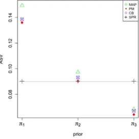
an illustration of Theorem3.1. It is also of interest to note that as we observe from Fig.3, the CB estimator is the only estimator with the same distribution of the posterior distribution of the parameters (the corresponding histogram and histogram of PESV fall on each other). Further, Fig.4provides averages of PESV (APESV) of ensemble of the parameters inθ52 and ASV of ensemble of

the different estimates w.r.t. all the priorsπj,j= 1,2,3 given by Eq. (5.3). This

figure also confirms that PESV associated with each of the priorsπj,j= 1,2,3,

is always greater than sample variance of the corresponding PM estimates (as provided by Lemma 3.1), and the CB estimator is the only estimator of which the corresponding sample variance is equal to the PESV of ensemble of the parameters inθ52(as an illustration of Theorem3.1).

On the other hand, if δ5l estimatesθ5l very well, the corresponding ASV is

expected to be close to 1₂(θ51l−1₂)2+ (θ52l−1₂)2

, which is equal to 0.01 for

l = 1 and 0.09 forl= 2. From Fig.4 we observe that the ASV of the SPRGM estimates of θ52 is not close to the APESV but its ASV is very close to 0.09.

Also, this is clearly observed from Fig. 3 in which the histogram of SPRGM estimates is centred about 0.09. Comparing the PM and the CB estimates, we observe that ASV of the CB estimates w.r.t. the priorπ3is closer to 0.09 than

the corresponding PM estimates and thus, their performance is better than the PM estimates w.r.t. the priors π3. This also can be confirmed from Table 1.

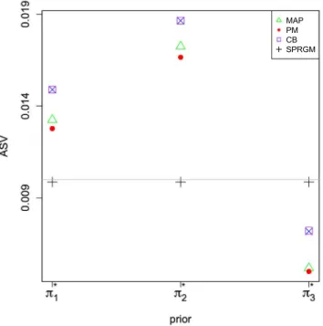
Thus, in some situations, the CB estimates act better than the PM ones. The same conclusions are deduced when estimating the parametersθ5i1,i=

1,2, w.r.t the priors π_j∗, j = 1,2,3, and the class of priors Γ∗, see Table A.1, Fig.A.1and Fig.A.2of the Appendix.

5.2. Real clinical data

4016

Fig 3_{. Histograms of ASV of ensemble of the MAP, PM, CB estimates w.r.t. the priorsπj,}

j = 1,2,3, and SPRGM estimates w.r.t. the class of priorsΓ along with histograms of the PESV of ensemble of the parameters in θ52. Each row is associated with one of the priors

4017

Fig 4_{. Plots of ASV of the MAP, PM, CB estimates w.r.t. the priorsπj, j = 1,2,3, and}

SPRGM estimates w.r.t. the class of priors Γ along with the APESV of ensemble of the parameters inθ52. In the figure,×represents PSEV. Also, green triangle corresponds to ASV

of the MAP estimates, red dot refers to ASV of the PM estimates, purple square represents ASV of the CB estimates, and black plus sign corresponds to ASV of the SPRGM estimates.

Fig 5. The structure of the Hepar BN.

The network models 18 variables related to diagnosis of a small set of hepatic disorders: three risk factors, 12 symptoms and test results, and three disorder nodes. To give the reader an idea of the number of numerical parameters needed to quantify a BN, let us assume for simplicity that each variable in the model in Fig.5 is Binary.

4018

Fig 6_{. Simplified Hepar BN model.}

values that pertain to PBC in some way. We will use this as an example to examine the effects of different parameter estimation methods. For example, LE cells = 0 and Antimytochondrial AB = 1, Gender = female will already give a high probability if the Age is above 40 and these are indeed part of the characteristics of the disease according to the clinical literature.

For simplicity, we refer to PBC, LE cells, Antimytochondrial AB, Gender and Age byB,L,A,GandE, respectively. The variablesA,GandLare assumed to be binary. For the variable Age, we consider thatEtakes value 0 if the patient’s age is under 40 and takes value 1, otherwise. Also, in our clinical data,B takes either the value zero (disease is absent) or one (disease is present). Thus, our goal is to compute

P(B = 1|G= 0, E= 1, L= 0, A= 1). (5.4)

Fig. 6 shows a simplified Hepar BN network with only these variables in-cluded. The following lemma restates the probability in (5.4) in terms of θjil

defined in Eq. (2.2).

Lemma 5.1. If we replaceG, E, B, L, A by the variablesX1, . . . , X5 and their

associated probabilistic parameters, the desired probability in (5.4) can be ex-pressed as follows

P(B = 1|G= 0, E= 1, L= 0, A= 1) = θ412θ522θ322

θ411θ521θ312+θ412θ522θ322

=θD.(5.5)

Suppose we know that the probabilityθ312=P(B= 1|E >40, A= 0) has a

high value (from our prior experience), but we are unable to determine its exact value reliably based on the data available. From the data we first determine point estimates for the parameters in Eq. (5.5), i.e., we can at least propose a prior distribution by looking at possible estimates ofθ312, e.g. its ML estimate,

which is 0.883. Based on this value, one may consider using theDir(α312, α322

)-prior withα312= 50 andα322= 5, which gives a prior mean of 50/55=0.9091.

4019

below, which reflects the possibility of getting some estimates in the interval (40/48, 60/62).

By expressing the uncertainty of the parameters in terms of some classes of conjugate distributions as listed below, we make sure that a wider range of probabilities is covered.

Γ1 =

Dir(α312, α322) : 40≤α312≤60,2≤α322≤8

,

Γ2 =

Dir(α411, α421) : 5≤α411≤25,90≤α421≤110

,

Γ3 =

Dir(α412, α422) : 2≤α412≤8,5≤α422≤15

,

Γ4 =

Dir(α511, α521) : 90≤α511≤110,2≤α522≤4

,

Γ5 =

Dir(α512, α522) : 3≤α512≤8,3≤α522≤8

.

One way to derive the SPRGM estimate of θD, is to compute SPRGM

esti-mate for each ofθjilas appeared in Eq. (5.5). The relevant computed estimates

are shown in Table2. It can be observed that the SPRGM estimate of the de-sired parameter θD is high enough, as somehow expected. For comparison, we

also report on the corresponding ML estimates in Table2. It should be empha-sized that since ML estimates do not depend on the prior knowledge, comparing ML estimates and Bayesian estimates is not fair and we should rely on the ML estimates only in situations in which we do not have access to any source of prior information.

Table 2

Computed SPRGM estimates of the parameters appeared in the Eq. (5.5).

Estimates θ312 θ322 θ411 θ412 θ521 θ522 θD

ML 0.8830 0.1170 0.1316 0.3071 0.0120 0.5679 0.9362 SPRGM 0.8889 0.1111 0.1317 0.3086 0.0200 0.0246 0.9150

6. Final remarks

4020

in the literature and new developments have been introduced, see for example [17] among many others. Thus assuming the random variables are discrete is not a restrictive assumption.

We also highlight that in our developments we assumed a BN with a complete instantiation is available, meaning that no missing values are present. But we would like to emphasize that in the presence of incomplete/missing data it can be handled with one of the available methods in the literature. [8] provided a theoretical approach to handle the problem of learning with missing data. They show that one can solve this problem by taking a sum of the conditional probabilities over all posible values for each missing data point. [27] studied the parameter learning task in presence of some missing data based on the Expectation-Maximization (EM) technique. [36] applied the important sampling technique into solving such a problem.

Among the existing methods, we suggest using the EM algorithm due to its advantage of being easy to implement and having the property of converging relatively quickly [38].

Now, to apply the EM algorithm, suppose that in the kth sample, k = 1,2, . . . , n, of the variables in the set x(k), Xm is the variable whose value is

missing. The EM algorithm starts with an initial estimationθ0 and at each

it-eration t, the data set is completed based on θt and then the parameters are

re-estimated using the completed data set, obtainingθt+1. The E-step finds the

conditional expectation of the complete data log-likelihood, given the observed component of the data and the current values of the parameters. In fact, the E-step computes the current expected log-likelihood ofθ given the data x, as denoted byQ(θ|θt) for simplicity below

Q(θ|θt) =

k

xm

P(Xm=xm|X(k)=x(k), θt) logP(X(k)=x(k), Xm=i|θ)

=

k

xm

i

j

l

P(Xm=xm|X(k)=x(k), θt)njilklogθjil

=

i

j

l

mtjillogθjil,

wheremt_jil=_kxmP(Xm=xm|X(k)=x(k), θt)njilkin whichnjilkis given

by the Eq. (2.1).

The M-step then computes the next estimate θt by maximizing the current

expected log-likelihood of the data, i.e., θt+1 = arg maxθQ(θ|θt). After some

algebraic manipulations, for alli,j andk, we will get

θt_jil+1= m

t jil

imtjil

.

Here mt

jil is interpreted as the number of cases where Xj =i when its parent

configuration is in the state λl in the completed data set. Thus, θtjil+1 is

inter-preted as the expected proportion of cases whereXj=iamong all possibilities

4021

Since the EM algorithm converges [26,38], this iterative approach leads to a replacement ofθjilbyθsjil, where sis the time thereafterθtjilis constant. Once

this replacement is done,δ_jilM Lin Eq. (2.3) is derived. Sincenj.l.will be known, we

getnjil.=δjilM Lnj.l.. Now, replacing the new value fornjil.in Eq. (2.5) and Eq.

(2.6), as well as Theorems3.1,4.1and4.2leads to MAP, PM, CB, and SPRGM estimates of parameters associated with the variable whose value is missing.

7. Conclusions and discussion

In this paper we considered the task of parameter learning in BNs. Improvements of Bayesian methods were provided, leading to the extension and application of the simultaneous estimation and robust Bayesian methodology to the context of parameter learning in BNs.

Assuming accessibility of some prior knowledge, we dealt with different ap-proaches to incorporate prior knowledge and derived explicit forms of Bayes (MAP and PM), adjusted Bayes (CB) and robust Bayes (SPRGM) estimates. From the Bayesian estimation literature it is understood that, in presence of crisp prior knowledge, one can reach a reliable Bayes estimate for the desired parameter. Prior knowledge can be specified by determining hyperparameters of the underlying prior distribution, but in many situations there may be a lack of consensus among experts or decision-makers concerning these hyperparame-ters. In such situations, one sensible approach, as adopted in this paper, would be to define a class of priors to ensure that the existing knowledge fall within the proposed class. The corresponding rule, which we referred to as the ‘robust Bayes rule’, can be used in the hope of arriving at a rule consistent with the real world.

Our simulation study emphasizes that if the crisp prior is present, Bayes and CB rules are reliable methods. This was obvious from the choiceDir(40,10) and

Dir(35,10)-priors and the corresponding Bayes and CB estimates in TableA.1 of the Appendix, as the true parameter was 0.2 and 0.4, respectively. But it is seen that for the other specified priors, the resulting Bayes and CB estimates are quite far from the true parameters and thus, these selected priors are bad choices. However, as noted earlier in the simulation study, in practice, the avail-ability of exact prior knowledge in terms of specific prior hyperparameters is rare. The overall class (5.1) was rich enough to ensure that it includes all the prior information attributed by the three experts. In addition to prevention of selecting bad choices of priors, quantitative statistics show that the SPRGM estimates perform quite well.

4022

PM estimates. We encourage using the CB estimates only if the interest lies in both simultaneous estimation and closeness between distribution of estimates and posterior distribution of the parameters. When there is a lack of consensus of opinion about the prior hyperparameters, we encourage using the SPRGM estimate(s), with the hope of reaching an optimal estimate.

We would like to wrap up this work by addressing the main interest of Bayesian analysis considered in this paper. Although different prior-based point estimates of the desired parameters have been provided in this paper, the points estimates have been driven by recovering the posterior distribution. The MAP and PM rules are the points that minimize the posterior function which is infor-mally averages of losses of choosing an estimator of the desired parameter w.r.t. the posterior distribution, the CB estimates adjust the PM estimates according to the additional constraints (i)-(iii) of Section 3 and the SPRGM estimates minimize the difference between posterior risk of any arbitrary estimator and the posterior risk of the Bayes estimator.

Appendix

Proof of Lemma 3.1.

E

kj

i=1

θjil−θ¯j.l

2

|X =x

=

kj

i=1

E[θ_jil2 |X=x]−kjE[¯θj.l2 |X=x]

=

kj

i=1

E[θ_jil2 |X=x]−kjV ar[¯θj.l|X=x]−kjE2[¯θj.l|X =x]

=

kj

i=1

E[θ_jil2 |X=x]− 1

kj

(since ¯θj.l=

1

kj

)

>

kj

i=1

E2[θjil|X=x]−

1

kj

(by Jensen inequality)

=

kj

i=1

E2[θjil|X=x]−kjδ¯P M

2

jl (since ¯δP Mjl =

1

kj kj

i=1

δ_jilP M = 1

kj

)

=

kj

i=1

δP Mjil 2−kjδ¯P M

2

j.l

=

kj

i=1

δP M_jil −δ¯P M_j.l 2.

4023

E

kj

i=1

θjil−θ¯j.l

2

|X =x

> kj i=1

δP M_jil −δ¯P M_jl 2.

Proof of Theorem 3.1. To derive CB estimates of the elements of θjl, we

minimize

E

kj

i=1

(θjil−δjil)2|X=x

,

w.r.t.δjilsubject to (i)-(iii). First note that

E

kj

i=1

(θjil−δjil)2|X =x

= E

kj

i=1

θjil+δP Mjil −δjilP M−δjil

2

|X=x

= E

kj

i=1

θjil−δP Mjil

2

|X=x

+ kj i=1

δjil−δjilP M

2

. (A.1)

The first term in the RHS of (A.1) does not depend on the estimatesδjil. Hence,

minimizing E[kj_i=1(θjil−δjil)2|X = x] subject to the constraints (i)-(iii) is

equivalent to minimizingkj_i=1

δjil−δjilP M

2

subject to the conditions (i)-(iii).

From the constraint (i),kj_i=1δjil=

kj

i=1δP Mjil , we observe that

kj

i=1

δjil−δjilP M

2 = kj i=1

δjil−¯δj.l+ ¯δj.lP M−δjilP M

2 = kj i=1

δjil−¯δj.l

2 + kj i=1

δP M_jil −δ¯P M_j.l 2

−2

kj

i=1

δP M_jil −δ¯P M_j.l δjil−δ¯j.l

= kj(V ar(Zjl) +V ar(Wjl)−2Cov(Zjl, Wjl)),(A.2)

where for a fixedj= 1, . . . , dandl= 1, . . . , qj,

P(Zjl=δjil, Wjl=δjilP M) =

1

kj

, i= 1, . . . , kj.

Due to the constraint (ii), for a fixedj = 1, . . . , dandl= 1, . . . , qj,V ar(Zjl) is

constant. It is obvious thatV ar(Wjl) does not depend onδjilvalues. Thus, the

right side of (A.2) is minimized whenCov(Zjl, Wjl) =

V ar(Zjl)

V ar(Wjl) or

equivalently the corresponding correlation is equal to one, i.e.,ρ(Zjl, Wjl) = 1.

This implies that Wjl =ajlZjl+bjl with probability 1 for some ajl >0 and

bjl∈ . Thus,

δjil = ajlδP Mjil +bjl. (A.3)