A Tutorial on Spectral Clustering
Ulrike von Luxburg
Max Planck Institute for Biological Cybernetics
Spemannstr. 38, 72076 T¨
ubingen, Germany
[email protected]
This article appears in Statistics and Computing, 17 (4), 2007.The original publication is available atwww.springer.com.
Abstract
In recent years, spectral clustering has become one of the most popular modern clustering algorithms. It is simple to implement, can be solved efficiently by standard linear algebra software, and very often outperforms traditional clustering algorithms such as the k-means algorithm. On the first glance spectral clustering appears slightly mysterious, and it is not obvious to see why it works at all and what it really does. The goal of this tutorial is to give some intuition on those questions. We describe different graph Laplacians and their basic properties, present the most common spectral clustering algorithms, and derive those algorithms from scratch by several different approaches. Advantages and disadvantages of the different spectral clustering algorithms are discussed.
Keywords: spectral clustering; graph Laplacian
1
Introduction
Clustering is one of the most widely used techniques for exploratory data analysis, with applications ranging from statistics, computer science, biology to social sciences or psychology. In virtually every scientific field dealing with empirical data, people attempt to get a first impression on their data by trying to identify groups of “similar behavior” in their data. In this article we would like to introduce the reader to the family of spectral clustering algorithms. Compared to the “traditional algorithms”
such ask-means or single linkage, spectral clustering has many fundamental advantages. Results
ob-tained by spectral clustering often outperform the traditional approaches, spectral clustering is very simple to implement and can be solved efficiently by standard linear algebra methods.
This tutorial is set up as a self-contained introduction to spectral clustering. We derive spectral clustering from scratch and present different points of view to why spectral clustering works. Apart from basic linear algebra, no particular mathematical background is required by the reader. However, we do not attempt to give a concise review of the whole literature on spectral clustering, which is
impossible due to the overwhelming amount of literature on this subject. The first two sections
are devoted to a step-by-step introduction to the mathematical objects used by spectral clustering: similarity graphs in Section 2, and graph Laplacians in Section 3. The spectral clustering algorithms themselves will be presented in Section 4. The next three sections are then devoted to explaining why those algorithms work. Each section corresponds to one explanation: Section 5 describes a graph partitioning approach, Section 6 a random walk perspective, and Section 7 a perturbation theory approach. In Section 8 we will study some practical issues related to spectral clustering, and discuss various extensions and literature related to spectral clustering in Section 9.
2
Similarity graphs
Given a set of data points x1, . . . xn and some notion of similaritysij ≥0 between all pairs of data
pointsxi andxj, the intuitive goal of clustering is to divide the data points into several groups such
that points in the same group are similar and points in different groups are dissimilar to each other. If we do not have more information than similarities between data points, a nice way of representing the
data is in form of thesimilarity graphG= (V, E). Each vertexviin this graph represents a data point
xi. Two vertices are connected if the similaritysij between the corresponding data pointsxi andxjis
positive or larger than a certain threshold, and the edge is weighted bysij. The problem of clustering
can now be reformulated using the similarity graph: we want to find a partition of the graph such that the edges between different groups have very low weights (which means that points in different clusters are dissimilar from each other) and the edges within a group have high weights (which means that points within the same cluster are similar to each other). To be able to formalize this intuition we first want to introduce some basic graph notation and briefly discuss the kind of graphs we are going to study.
2.1
Graph notation
LetG= (V, E) be an undirected graph with vertex setV ={v1, . . . , vn}. In the following we assume
that the graphGis weighted, that is each edge between two verticesvi andvj carries a non-negative
weight wij ≥ 0. The weighted adjacency matrix of the graph is the matrix W = (wij)i,j=1,...,n. If
wij = 0 this means that the verticesvi andvj are not connected by an edge. AsG is undirected we
requirewij=wji. The degree of a vertexvi∈V is defined as
di= n
X
j=1
wij.
Note that, in fact, this sum only runs over all vertices adjacent tovi, as for all other vertices vj the
weight wij is 0. The degree matrix D is defined as the diagonal matrix with the degrees d1, . . . , dn
on the diagonal. Given a subset of vertices A ⊂ V, we denote its complement V \A by A. We
define the indicator vector 1A = (f1, . . . , fn)0 ∈ Rn as the vector with entries fi = 1 if vi ∈ A and
fi = 0 otherwise. For convenience we introduce the shorthand notation i∈A for the set of indices
{i|vi∈A}, in particular when dealing with a sum likePi∈Awij. For two not necessarily disjoint sets
A, B⊂V we define
W(A, B) := X
i∈A,j∈B
wij.
We consider two different ways of measuring the “size” of a subsetA⊂V:
|A|:= the number of vertices inA
vol(A) :=X
i∈A
di.
Intuitively,|A| measures the size ofA by its number of vertices, while vol(A) measures the size ofA
by summing over the weights of all edges attached to vertices in A. A subset A ⊂V of a graph is
connected if any two vertices in Acan be joined by a path such that all intermediate points also lie
in A. A subset A is called a connected component if it is connected and if there are no connections
between vertices inAandA. The nonempty setsA1, . . . , Akform a partition of the graph ifAi∩Aj=∅
2.2
Different similarity graphs
There are several popular constructions to transform a given setx1, . . . , xn of data points with pairwise
similaritiessij or pairwise distancesdij into a graph. When constructing similarity graphs the goal is
to model the local neighborhood relationships between the data points.
Theε-neighborhood graph: Here we connect all points whose pairwise distances are smaller thanε.
As the distances between all connected points are roughly of the same scale (at mostε), weighting the
edges would not incorporate more information about the data to the graph. Hence, theε-neighborhood
graph is usually considered as an unweighted graph.
k-nearest neighbor graphs: Here the goal is to connect vertex vi with vertex vj if vj is among
thek-nearest neighbors ofvi. However, this definition leads to a directed graph, as the neighborhood
relationship is not symmetric. There are two ways of making this graph undirected. The first way is
to simply ignore the directions of the edges, that is we connectviandvj with an undirected edge ifvi
is among thek-nearest neighbors ofvj orifvj is among thek-nearest neighbors ofvi. The resulting
graph is what is usually calledthe k-nearest neighbor graph. The second choice is to connect vertices
vi andvj if bothvi is among thek-nearest neighbors of vj andvj is among thek-nearest neighbors of
vi. The resulting graph is called themutualk-nearest neighbor graph. In both cases, after connecting
the appropriate vertices we weight the edges by the similarity of their endpoints.
The fully connected graph: Here we simply connect all points with positive similarity with each
other, and we weight all edges by sij. As the graph should represent the local neighborhood
re-lationships, this construction is only useful if the similarity function itself models local
neighbor-hoods. An example for such a similarity function is the Gaussian similarity function s(xi, xj) =
exp(−kxi−xjk2/(2σ2)), where the parameterσ controls the width of the neighborhoods. This
pa-rameter plays a similar role as the papa-rameterεin case of theε-neighborhood graph.
All graphs mentioned above are regularly used in spectral clustering. To our knowledge, theoretical results on the question how the choice of the similarity graph influences the spectral clustering result do not exist. For a discussion of the behavior of the different graphs we refer to Section 8.
3
Graph Laplacians and their basic properties
The main tools for spectral clustering are graph Laplacian matrices. There exists a whole field ded-icated to the study of those matrices, called spectral graph theory (e.g., see Chung, 1997). In this section we want to define different graph Laplacians and point out their most important properties. We will carefully distinguish between different variants of graph Laplacians. Note that in the literature there is no unique convention which matrix exactly is called “graph Laplacian”. Usually, every author just calls “his” matrix the graph Laplacian. Hence, a lot of care is needed when reading literature on graph Laplacians.
In the following we always assume that G is an undirected, weighted graph with weight matrixW,
wherewij =wji≥0. When using eigenvectors of a matrix, we will not necessarily assume that they
are normalized. For example, the constant vector1and a multiplea1for somea6= 0 will be considered
as the same eigenvectors. Eigenvalues will always be ordered increasingly, respecting multiplicities.
3.1
The unnormalized graph Laplacian
The unnormalized graph Laplacian matrix is defined as
L=D−W.
An overview over many of its properties can be found in Mohar (1991, 1997). The following proposition summarizes the most important facts needed for spectral clustering.
Proposition 1 (Properties ofL) The matrixL satisfies the following properties:
1. For every vectorf ∈Rn we have
f0Lf =1 2
n
X
i,j=1
wij(fi−fj)2.
2. Lis symmetric and positive semi-definite.
3. The smallest eigenvalue of Lis 0, the corresponding eigenvector is the constant one vector 1.
4. Lhas nnon-negative, real-valued eigenvalues 0 =λ1≤λ2≤. . .≤λn.
Proof.
Part (1): By the definition ofdi,
f0Lf =f0Df−f0W f=
n
X
i=1
difi2− n
X
i,j=1
fifjwij
=1
2
n
X
i=1
difi2−2 n
X
i,j=1
fifjwij+ n
X
j=1
djfj2
=
1 2
n
X
i,j=1
wij(fi−fj)2.
Part (2): The symmetry ofL follows directly from the symmetry of W and D. The positive
semi-definiteness is a direct consequence of Part (1), which shows thatf0Lf ≥0 for allf ∈Rn.
Part (3): Obvious.
Part (4) is a direct consequence of Parts (1) - (3). 2
Note that the unnormalized graph Laplacian does not depend on the diagonal elements of the
adja-cency matrixW. Each adjacency matrix which coincides with W on all off-diagonal positions leads
to the same unnormalized graph LaplacianL. In particular, self-edges in a graph do not change the
corresponding graph Laplacian.
The unnormalized graph Laplacian and its eigenvalues and eigenvectors can be used to describe many properties of graphs, see Mohar (1991, 1997). One example which will be important for spectral clustering is the following:
Proposition 2 (Number of connected components and the spectrum ofL) LetGbe an
undi-rected graph with non-negative weights. Then the multiplicity k of the eigenvalue 0 of L equals the
number of connected componentsA1, . . . , Ak in the graph. The eigenspace of eigenvalue 0 is spanned
by the indicator vectors1A1, . . . ,1Ak of those components.
Proof. We start with the casek= 1, that is the graph is connected. Assume thatf is an eigenvector
with eigenvalue 0. Then we know that
0 =f0Lf =
n
X
i,j=1
As the weightswij are non-negative, this sum can only vanish if all termswij(fi−fj)2vanish. Thus,
if two verticesvi andvj are connected (i.e.,wij >0), thenfi needs to equalfj. With this argument
we can see thatf needs to be constant for all vertices which can be connected by a path in the graph.
Moreover, as all vertices of a connected component in an undirected graph can be connected by a
path, f needs to be constant on the whole connected component. In a graph consisting of only one
connected component we thus only have the constant one vector1 as eigenvector with eigenvalue 0,
which obviously is the indicator vector of the connected component.
Now consider the case of k connected components. Without loss of generality we assume that the
vertices are ordered according to the connected components they belong to. In this case, the adjacency
matrixW has a block diagonal form, and the same is true for the matrixL:
L=
L1
L2
. ..
Lk
Note that each of the blocksLi is a proper graph Laplacian on its own, namely the Laplacian
corre-sponding to the subgraph of the i-th connected component. As it is the case for all block diagonal
matrices, we know that the spectrum ofL is given by the union of the spectra of Li, and the
corre-sponding eigenvectors ofLare the eigenvectors ofLi, filled with 0 at the positions of the other blocks.
As eachLi is a graph Laplacian of a connected graph, we know that every Li has eigenvalue 0 with
multiplicity 1, and the corresponding eigenvector is the constant one vector on the i-th connected
component. Thus, the matrixL has as many eigenvalues 0 as there are connected components, and
the corresponding eigenvectors are the indicator vectors of the connected components. 2
3.2
The normalized graph Laplacians
There are two matrices which are called normalized graph Laplacians in the literature. Both matrices are closely related to each other and are defined as
Lsym:=D−1/2LD−1/2=I−D−1/2W D−1/2
Lrw:=D−1L=I−D−1W.
We denote the first matrix byLsym as it is a symmetric matrix, and the second one by Lrw as it is
closely related to a random walk. In the following we summarize several properties ofLsym andLrw.
The standard reference for normalized graph Laplacians is Chung (1997).
Proposition 3 (Properties ofLsym and Lrw) The normalized Laplacians satisfy the following
prop-erties:
1. For everyf ∈Rn we have
f0Lsymf =
1 2
n
X
i,j=1
wij
fi
√
di
−pfj
dj
!2 .
2. λ is an eigenvalue of Lrw with eigenvector u if and only if λ is an eigenvalue of Lsym with
eigenvector w=D1/2u.
3. λis an eigenvalue of Lrw with eigenvector uif and only if λand usolve the generalized
4. 0 is an eigenvalue of Lrw with the constant one vector 1 as eigenvector. 0 is an eigenvalue of
Lsym with eigenvectorD1/21.
5. Lsym and Lrw are positive semi-definite and have n non-negative real-valued eigenvalues 0 =
λ1≤. . .≤λn.
Proof. Part (1) can be proved similarly to Part (1) of Proposition 1.
Part (2) can be seen immediately by multiplying the eigenvalue equation Lsymw =λw with D−1/2
from the left and substitutingu=D−1/2w.
Part (3) follows directly by multiplying the eigenvalue equationLrwu=λuwith Dfrom the left.
Part (4): The first statement is obvious asLrw1= 0, the second statement follows from (2).
Part (5): The statement aboutLsymfollows from (1), and then the statement aboutLrw follows from
(2). 2
As it is the case for the unnormalized graph Laplacian, the multiplicity of the eigenvalue 0 of the normalized graph Laplacian is related to the number of connected components:
Proposition 4 (Number of connected components and spectra ofLsym and Lrw) Let G be
an undirected graph with non-negative weights. Then the multiplicitykof the eigenvalue0 of bothLrw
andLsymequals the number of connected componentsA1, . . . , Ak in the graph. ForLrw, the eigenspace
of 0 is spanned by the indicator vectors 1Ai of those components. For Lsym, the eigenspace of 0 is
spanned by the vectorsD1/21
Ai.
Proof. The proof is analogous to the one of Proposition 2, using Proposition 3. 2
4
Spectral Clustering Algorithms
Now we would like to state the most common spectral clustering algorithms. For references and the
history of spectral clustering we refer to Section 9. We assume that our data consists ofn “points”
x1, . . . , xn which can be arbitrary objects. We measure their pairwise similarities sij = s(xi, xj)
by some similarity function which is symmetric and non-negative, and we denote the corresponding similarity matrix byS = (sij)i,j=1...n.
Unnormalized spectral clustering Input: Similarity matrix S∈Rn×n
, number k of clusters to construct.
• Construct a similarity graph by one of the ways described in Section 2. Let W be its weighted adjacency matrix.
• Compute the unnormalized Laplacian L.
• Compute the firstk eigenvectors u1, . . . , uk of L.
• Let U ∈Rn×k
be the matrix containing the vectors u1, . . . , uk as columns.
• For i= 1, . . . , n, let yi ∈Rk be the vector corresponding to the i-th row of U.
• Cluster the points (yi)i=1,...,n in Rk with the k-means algorithm into clusters
C1, . . . , Ck.
Output: Clusters A1, . . . , Ak with Ai={j|yj∈Ci}.
graph Laplacians is used. We name both algorithms after two popular papers, for more references and history please see Section 9.
Normalized spectral clustering according to Shi and Malik (2000) Input: Similarity matrix S∈Rn×n
, number k of clusters to construct.
• Construct a similarity graph by one of the ways described in Section 2. Let W be its weighted adjacency matrix.
• Compute the unnormalized Laplacian L.
• Compute the first k generalized eigenvectors u1, . . . , uk of the generalized
eigenprob-lem Lu=λDu.
• Let U ∈Rn×k
be the matrix containing the vectors u1, . . . , uk as columns.
• For i= 1, . . . , n, let yi ∈Rk be the vector corresponding to the i-th row of U.
• Cluster the points (yi)i=1,...,n in Rk with the k-means algorithm into clusters
C1, . . . , Ck.
Output: Clusters A1, . . . , Ak with Ai={j|yj∈Ci}.
Note that this algorithm uses the generalized eigenvectors of L, which according to Proposition 3
correspond to the eigenvectors of the matrixLrw. So in fact, the algorithm works with eigenvectors of
the normalized LaplacianLrw, and hence is called normalized spectral clustering. The next algorithm
also uses a normalized Laplacian, but this time the matrixLsym instead ofLrw. As we will see, this
algorithm needs to introduce an additional row normalization step which is not needed in the other algorithms. The reasons will become clear in Section 7.
Normalized spectral clustering according to Ng, Jordan, and Weiss (2002) Input: Similarity matrix S∈Rn×n
, number k of clusters to construct.
• Construct a similarity graph by one of the ways described in Section 2. Let W be its weighted adjacency matrix.
• Compute the normalized Laplacian Lsym.
• Compute the firstk eigenvectors u1, . . . , uk of Lsym.
• Let U ∈Rn×k
be the matrix containing the vectors u1, . . . , uk as columns.
• Form the matrix T ∈Rn×k from U by normalizing the rows to norm 1,
that is set tij =uij/(Pku
2
ik)
1/2.
• For i= 1, . . . , n, let yi ∈Rk be the vector corresponding to the i-th row of T.
• Cluster the points (yi)i=1,...,n with the k-means algorithm into clusters C1, . . . , Ck.
Output: Clusters A1, . . . , Ak with Ai={j|yj∈Ci}.
All three algorithms stated above look rather similar, apart from the fact that they use three different graph Laplacians. In all three algorithms, the main trick is to change the representation of the abstract
data pointsxito pointsyi∈Rk. It is due to the properties of the graph Laplacians that this change of
representation is useful. We will see in the next sections that this change of representation enhances the cluster-properties in the data, so that clusters can be trivially detected in the new representation.
In particular, the simplek-means clustering algorithm has no difficulties to detect the clusters in this
0 2 4 6 8 10 0 2 4 6 8
Histogram of the sample
1 2 3 4 5 6 7 8 9 10 0 0.02 0.04 0.06 0.08 Eigenvalues norm, knn
2 4 6 8 0
0.2 0.4
norm, knn
Eigenvector 1
2 4 6 8 −0.5 −0.4 −0.3 −0.2 −0.1 Eigenvector 2
2 4 6 8 0
0.2 0.4
Eigenvector 3
2 4 6 8 0
0.2 0.4
Eigenvector 4
2 4 6 8 −0.5
0 0.5
Eigenvector 5
1 2 3 4 5 6 7 8 9 10 0 0.01 0.02 0.03 0.04 Eigenvalues unnorm, knn
2 4 6 8 0
0.05 0.1
unnorm, knn
Eigenvector 1
2 4 6 8 −0.1
−0.05 0
Eigenvector 2
2 4 6 8 −0.1
−0.05 0
Eigenvector 3
2 4 6 8 −0.1
−0.05 0
Eigenvector 4
2 4 6 8 −0.1
0 0.1
Eigenvector 5
1 2 3 4 5 6 7 8 9 10 0 0.2 0.4 0.6 0.8 Eigenvalues
norm, full graph
2 4 6 8 −0.1451
−0.1451 −0.1451
norm, full graph
Eigenvector 1
2 4 6 8 −0.1
0 0.1
Eigenvector 2
2 4 6 8 −0.1
0 0.1
Eigenvector 3
2 4 6 8 −0.1
0 0.1
Eigenvector 4
2 4 6 8 −0.5
0 0.5
Eigenvector 5
1 2 3 4 5 6 7 8 9 10 0
0.05 0.1 0.15
Eigenvalues
unnorm, full graph
2 4 6 8 −0.0707
−0.0707 −0.0707
unnorm, full graph
Eigenvector 1
2 4 6 8 −0.05
0 0.05
Eigenvector 2
2 4 6 8 −0.05
0 0.05
Eigenvector 3
2 4 6 8 −0.05
0 0.05
Eigenvector 4
2 4 6 8 0 0.2 0.4 0.6 0.8 Eigenvector 5
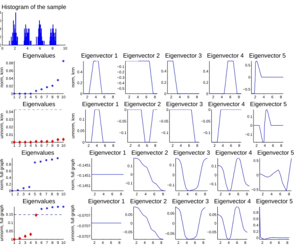
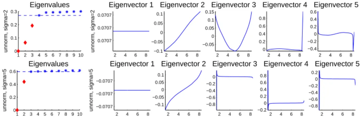
Figure 1: Toy example for spectral clustering where the data points have been drawn from a mixture of
four Gaussians onR. Left upper corner: histogram of the data. First and second row: eigenvalues and
eigenvectors ofLrw andLbased on the k-nearest neighbor graph. Third and fourth row: eigenvalues
and eigenvectors ofLrwandLbased on the fully connected graph. For all plots, we used the Gaussian
kernel withσ= 1 as similarity function. See text for more details.
text books, for example in Hastie, Tibshirani, and Friedman (2001).
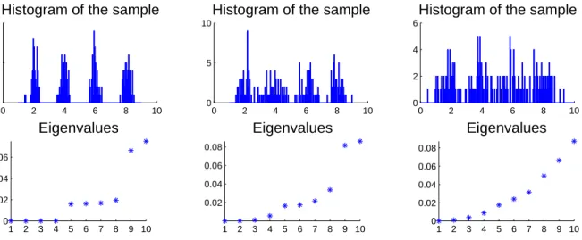
Before we dive into the theory of spectral clustering, we would like to illustrate its principle on a very simple toy example. This example will be used at several places in this tutorial, and we chose it because it is so simple that the relevant quantities can easily be plotted. This toy data set consists of a random
sample of 200 pointsx1, . . . , x200∈Rdrawn according to a mixture of four Gaussians. The first row
of Figure 1 shows the histogram of a sample drawn from this distribution (thex-axis represents the
one-dimensional data space). As similarity function on this data set we choose the Gaussian similarity functions(xi, xj) = exp(−|xi −xj|2/(2σ2)) with σ = 1. As similarity graph we consider both the
fully connected graph and the 10-nearest neighbor graph. In Figure 1 we show the first eigenvalues
and eigenvectors of the unnormalized LaplacianLand the normalized LaplacianLrw. That is, in the
eigenvalue plot we plotivs. λi (for the moment ignore the dashed line and the different shapes of the
eigenvalues in the plots for the unnormalized case; their meaning will be discussed in Section 8.5). In the eigenvector plots of an eigenvectoru= (u1, . . . , u200)0 we plotxi vs. ui (note that in the example
chosenxi is simply a real number, hence we can depict it on thex-axis). The first two rows of Figure
1 show the results based on the 10-nearest neighbor graph. We can see that the first four eigenvalues are 0, and the corresponding eigenvectors are cluster indicator vectors. The reason is that the clusters
form disconnected parts in the 10-nearest neighbor graph, in which case the eigenvectors are given as in Propositions 2 and 4. The next two rows show the results for the fully connected graph. As the Gaussian similarity function is always positive, this graph only consists of one connected component. Thus, eigenvalue 0 has multiplicity 1, and the first eigenvector is the constant vector. The following eigenvectors carry the information about the clusters. For example in the unnormalized case (last row), if we threshold the second eigenvector at 0, then the part below 0 corresponds to clusters 1 and 2, and the part above 0 to clusters 3 and 4. Similarly, thresholding the third eigenvector separates clusters 1 and 4 from clusters 2 and 3, and thresholding the fourth eigenvector separates clusters 1 and 3 from clusters 2 and 4. Altogether, the first four eigenvectors carry all the information about the
four clusters. In all the cases illustrated in this figure, spectral clustering usingk-means on the first
four eigenvectors easily detects the correct four clusters.
5
Graph cut point of view
The intuition of clustering is to separate points in different groups according to their similarities. For data given in form of a similarity graph, this problem can be restated as follows: we want to find a par-tition of the graph such that the edges between different groups have a very low weight (which means that points in different clusters are dissimilar from each other) and the edges within a group have high weight (which means that points within the same cluster are similar to each other). In this section we will see how spectral clustering can be derived as an approximation to such graph partitioning problems.
Given a similarity graph with adjacency matrix W, the simplest and most direct way to construct
a partition of the graph is to solve the mincut problem. To define it, please recall the notation
W(A, B) := P
i∈A,j∈Bwij and A for the complement of A. For a given number k of subsets, the
mincut approach simply consists in choosing a partitionA1, . . . , Ak which minimizes
cut(A1, . . . , Ak) :=
1 2
k
X
i=1
W(Ai, Ai).
Here we introduce the factor 1/2 for notational consistency, otherwise we would count each edge twice
in the cut. In particular fork= 2, mincut is a relatively easy problem and can be solved efficiently,
see Stoer and Wagner (1997) and the discussion therein. However, in practice it often does not lead to satisfactory partitions. The problem is that in many cases, the solution of mincut simply separates one individual vertex from the rest of the graph. Of course this is not what we want to achieve in clustering, as clusters should be reasonably large groups of points. One way to circumvent this problem
is to explicitly request that the setsA1, . . . , Akare “reasonably large”. The two most common objective
functions to encode this are RatioCut (Hagen and Kahng, 1992) and the normalized cut Ncut (Shi
and Malik, 2000). In RatioCut, the size of a subsetAof a graph is measured by its number of vertices
|A|, while in Ncut the size is measured by the weights of its edges vol(A). The definitions are:
RatioCut(A1, . . . , Ak) :=
1 2
k
X
i=1
W(Ai, Ai)
|Ai|
=
k
X
i=1
cut(Ai, Ai)
|Ai|
Ncut(A1, . . . , Ak) :=
1 2
k
X
i=1
W(Ai, Ai)
vol(Ai)
=
k
X
i=1
cut(Ai, Ai)
vol(Ai)
.
Note that both objective functions take a small value if the clustersAi are not too small. In
partic-ular, the minimum of the functionPk
i=1(1/|Ai|) is achieved if all |Ai|coincide, and the minimum of
Pk
i=1(1/vol(Ai)) is achieved if all vol(Ai) coincide. So what both objective functions try to achieve is
that the clusters are “balanced”, as measured by the number of vertices or edge weights, respectively. Unfortunately, introducing balancing conditions makes the previously simple to solve mincut problem
become NP hard, see Wagner and Wagner (1993) for a discussion. Spectral clustering is a way to solve relaxed versions of those problems. We will see that relaxing Ncut leads to normalized spectral clustering, while relaxing RatioCut leads to unnormalized spectral clustering (see also the tutorial slides by Ding (2004)).
5.1
Approximating RatioCut for
k
= 2
Let us start with the case of RatioCut andk= 2, because the relaxation is easiest to understand in
this setting. Our goal is to solve the optimization problem min
A⊂VRatioCut(A, A). (1)
We first rewrite the problem in a more convenient form. Given a subsetA⊂V we define the vector
f = (f1, . . . , fn)0∈Rn with entries
fi =
q
|A|/|A| ifvi∈A
−
q
|A|/|A| ifvi∈A.
(2)
Now the RatioCut objective function can be conveniently rewritten using the unnormalized graph Laplacian. This is due to the following calculation:
f0Lf = 1 2
n
X
i,j=1
wij(fi−fj)2
= 1
2
X
i∈A,j∈A
wij
s
|A| |A|+
s
|A| |A|
2 +1 2 X
i∈A,j∈A
wij
− s
|A| |A| −
s
|A| |A|
2
= cut(A, A)
|A|
|A|+ |A| |A|+ 2
= cut(A, A)
|A|+|A|
|A| +
|A|+|A| |A|
=|V| ·RatioCut(A, A).
Additionally, we have
n
X
i=1
fi=
X
i∈A
s
|A| |A|−
X
i∈A
s
|A| |A| =|A|
s
|A| |A|− |A|
s
|A| |A| = 0.
In other words, the vectorf as defined in Equation (2) is orthogonal to the constant one vector 1.
Finally, note thatf satisfies
kfk2=
n
X
i=1
fi2=|A||A| |A|+|A|
|A|
|A| =|A|+|A|=n.
Altogether we can see that the problem of minimizing (1) can be equivalently rewritten as min
A⊂Vf
0Lf subject to f ⊥1, f
i as defined in Eq. (2), kfk=
√
n. (3)
This is a discrete optimization problem as the entries of the solution vectorf are only allowed to take
to discard the discreteness condition and instead allow thatfitakes arbitrary values inR. This leads
to the relaxed optimization problem min
f∈Rnf
0Lf subject tof ⊥1, kfk=√n. (4)
By the Rayleigh-Ritz theorem (e.g., see Section 5.5.2. of L¨utkepohl, 1997) it can be seen immediately
that the solution of this problem is given by the vectorf which is the eigenvector corresponding to
the second smallest eigenvalue ofL (recall that the smallest eigenvalue ofL is 0 with eigenvector1).
So we can approximate a minimizer of RatioCut by the second eigenvector ofL. However, in order
to obtain a partition of the graph we need to re-transform the real-valued solution vector f of the
relaxed problem into a discrete indicator vector. The simplest way to do this is to use the sign off as
indicator function, that is to choose
(
vi∈A iffi≥0
vi∈A iffi<0.
However, in particular in the case ofk > 2 treated below, this heuristic is too simple. What most
spectral clustering algorithms do instead is to consider the coordinates fi as points inRand cluster
them into two groups C, C by the k-means clustering algorithm. Then we carry over the resulting
clustering to the underlying data points, that is we choose
(
vi ∈A iffi∈C
vi ∈A iffi∈C.
This is exactly theunnormalized spectral clusteringalgorithm for the case of k= 2.
5.2
Approximating RatioCut for arbitrary
k
The relaxation of the RatioCut minimization problem in the case of a general valuekfollows a similar
principle as the one above. Given a partition ofV intoksetsA1, . . . , Ak, we definekindicator vectors
hj = (h1,j, . . . , hn,j)0 by
hi,j =
(
1/p|Aj| ifvi∈Aj
0 otherwise (i= 1, . . . , n; j = 1, . . . , k). (5)
Then we set the matrix H ∈ Rn×k as the matrix containing those k indicator vectors as columns.
Observe that the columns in H are orthonormal to each other, that is H0H = I. Similar to the
calculations in the last section we can see that
h0iLhi=
cut(Ai, Ai)
|Ai|
.
Moreover, one can check that
h0iLhi = (H0LH)ii.
Combining those facts we get
RatioCut(A1, . . . , Ak) = k
X
i=1
h0iLhi = k
X
i=1
where Tr denotes the trace of a matrix. So the problem of minimizing RatioCut(A1, . . . , Ak) can be
rewritten as
min
A1,...,AkTr(H
0LH) subject toH0H =I, H as defined in Eq. (5).
Similar to above we now relax the problem by allowing the entries of the matrixH to take arbitrary
real values. Then the relaxed problem becomes: min
H∈Rn×kTr(H
0LH) subject toH0H =I.
This is the standard form of a trace minimization problem, and again a version of the Rayleigh-Ritz
theorem (e.g., see Section 5.2.2.(6) of L¨utkepohl, 1997) tells us that the solution is given by choosing
H as the matrix which contains the firstkeigenvectors ofL as columns. We can see that the matrix
H is in fact the matrix U used in the unnormalized spectral clustering algorithm as described in
Section 4. Again we need to re-convert the real valued solution matrix to a discrete partition. As
above, the standard way is to use thek-means algorithms on the rows ofU. This leads to the general
unnormalized spectral clustering algorithm as presented in Section 4.
5.3
Approximating Ncut
Techniques very similar to the ones used for RatioCut can be used to derive normalized spectral
clustering as relaxation of minimizing Ncut. In the casek= 2 we define the cluster indicator vectorf
by
fi=
q
vol(A)
volA ifvi∈A
−qvol(A)
vol(A) ifvi∈A.
(6)
Similar to above one can check that (Df)01= 0,f0Df = vol(V), andf0Lf = vol(V) Ncut(A, A). Thus
we can rewrite the problem of minimizing Ncut by the equivalent problem min
A f
0Lf subject to f as in (6), Df ⊥1, f0Df = vol(V). (7)
Again we relax the problem by allowingf to take arbitrary real values:
min
f∈Rnf
0Lf subject to Df ⊥1, f0Df = vol(V). (8)
Now we substituteg:=D1/2f. After substitution, the problem is
min
g∈Rng
0D−1/2LD−1/2g subject to g⊥D1/21, kgk2= vol(V). (9)
Observe thatD−1/2LD−1/2=Lsym, D1/21 is the first eigenvector of Lsym, and vol(V) is a constant.
Hence, Problem (9) is in the form of the standard Rayleigh-Ritz theorem, and its solutiong is given
by the second eigenvector ofLsym. Re-substitutingf =D−1/2g and using Proposition 3 we see that
f is the second eigenvector ofLrw, or equivalently the generalized eigenvector ofLu=λDu.
For the case of findingk >2 clusters, we define the indicator vectorshj= (h1,j, . . . , hn,j)0 by
hi,j=
(
1/pvol(Aj) ifvi∈Aj
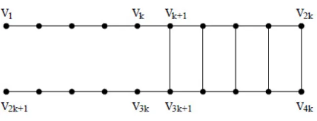
Figure 2: The cockroach graph from Guattery and Miller (1998).
Then we set the matrixH as the matrix containing thosekindicator vectors as columns. Observe that
H0H =I, h0iDhi = 1, andhi0Lhi = cut(Ai, Ai)/vol(Ai). So we can write the problem of minimizing
Ncut as
min
A1,...,Ak
Tr(H0LH) subject toH0DH =I, H as in (10).
Relaxing the discreteness condition and substitutingT =D1/2H we obtain the relaxed problem
min
T∈Rn×kTr(T
0D−1/2LD−1/2T) subject toT0T =I. (11)
Again this is the standard trace minimization problem which is solved by the matrixT which contains
the firstkeigenvectors ofLsymas columns. Re-substitutingH =D−1/2T and using Proposition 3 we
see that the solutionH consists of the firstkeigenvectors of the matrixLrw, or the firstkgeneralized
eigenvectors ofLu=λDu. This yields the normalized spectral clustering algorithm according to Shi
and Malik (2000).
5.4
Comments on the relaxation approach
There are several comments we should make about this derivation of spectral clustering. Most im-portantly, there is no guarantee whatsoever on the quality of the solution of the relaxed problem
compared to the exact solution. That is, ifA1, . . . , Akis the exact solution of minimizing RatioCut, and
B1, . . . , Bkis the solution constructed by unnormalized spectral clustering, then RatioCut(B1, . . . , Bk)−
RatioCut(A1, . . . , Ak) can be arbitrary large. Several examples for this can be found in Guattery
and Miller (1998). For instance, the authors consider a very simple class of graphs called
“cock-roach graphs”. Those graphs essentially look like a ladder, with a few rimes removed, see
Fig-ure 2. Obviously, the ideal RatioCut for k = 2 just cuts the ladder by a vertical cut such that
A={v1, . . . , vk, v2k+1, . . . , v3k}andA={vk+1, . . . , v2k, v3k+1, . . . , v4k}. This cut is perfectly balanced
with|A|=|A|= 2kand cut(A, A) = 2. However, by studying the properties of the second eigenvector
of the unnormalized graph Laplacian of cockroach graphs the authors prove that unnormalized spectral
clustering always cuts horizontally through the ladder, constructing the sets B = {v1, . . . , v2k} and
B ={v2k+1, . . . , v4k}. This also results in a balanced cut, but now we cut kedges instead of just 2.
So RatioCut(A, A) = 2/k, while RatioCut(B, B) = 1. This means that compared to the optimal cut,
the RatioCut value obtained by spectral clustering isk/2 times worse, that is a factor in the order of
n. Several other papers investigate the quality of the clustering constructed by spectral clustering, for
example Spielman and Teng (1996) (for unnormalized spectral clustering) and Kannan, Vempala, and Vetta (2004) (for normalized spectral clustering). In general it is known that efficient algorithms to approximate balanced graph cuts up to a constant factor do not exist. To the contrary, this approxi-mation problem can be NP hard itself (Bui and Jones, 1992).
Of course, the relaxation we discussed above is not unique. For example, a completely different relax-ation which leads to a semi-definite program is derived in Bie and Cristianini (2006), and there might be many other useful relaxations. The reason why the spectral relaxation is so appealing is not that it leads to particularly good solutions. Its popularity is mainly due to the fact that it results in a standard linear algebra problem which is simple to solve.
6
Random walks point of view
Another line of argument to explain spectral clustering is based on random walks on the similarity graph. A random walk on a graph is a stochastic process which randomly jumps from vertex to vertex. We will see below that spectral clustering can be interpreted as trying to find a partition of the graph such that the random walk stays long within the same cluster and seldom jumps between clusters. Intuitively this makes sense, in particular together with the graph cut explanation of the last section: a balanced partition with a low cut will also have the property that the random walk does not have many opportunities to jump between clusters. For background reading on random walks in general we
refer to Norris (1997) and Br´emaud (1999), and for random walks on graphs we recommend Aldous
and Fill (in preparation) and Lov´asz (1993). Formally, the transition probability of jumping in one
step from vertexvi to vertex vj is proportional to the edge weight wij and is given by pij :=wij/di.
The transition matrixP = (pij)i,j=1,...,n of the random walk is thus defined by
P =D−1W.
If the graph is connected and non-bipartite, then the random walk always possesses a unique stationary distributionπ= (π1, . . . , πn)0, whereπi=di/vol(V). Obviously there is a tight relationship between
LrwandP, asLrw=I−P. As a consequence,λis an eigenvalue ofLrw with eigenvectoruif and only
if 1−λis an eigenvalue ofP with eigenvectoru. It is well known that many properties of a graph can
be expressed in terms of the corresponding random walk transition matrixP, see Lov´asz (1993) for
an overview. From this point of view it does not come as a surprise that the largest eigenvectors ofP
and the smallest eigenvectors ofLrwcan be used to describe cluster properties of the graph.
Random walks and Ncut
A formal equivalence between Ncut and transition probabilities of the random walk has been observed in Meila and Shi (2001).
Proposition 5 (Ncut via transition probabilities) Let G be connected and non bi-partite.
As-sume that we run the random walk (Xt)t∈N starting with X0 in the stationary distribution π. For
disjoint subsetsA, B⊂V, denote byP(B|A) :=P(X1∈B|X0∈A). Then:
Ncut(A, A) =P(A|A) +P(A|A).
Proof. First of all observe that
P(X0∈A, X1∈B) =
X
i∈A,j∈B
P(X0=i, X1=j) =
X
i∈A,j∈B
πipij
= X
i∈A,j∈B
di
vol(V)
wij
di
= 1
vol(V)
X
i∈A,j∈B
Using this we obtain
P(X1∈B|X0∈A) =
P(X0∈A, X1∈B)
P(X0∈A)
=
1 vol(V)
X
i∈A,j∈B
wij
vol(A) vol(V)
−1
=
P
i∈A,j∈Bwij
vol(A) .
Now the proposition follows directly with the definition of Ncut. 2
This proposition leads to a nice interpretation of Ncut, and hence of normalized spectral clustering. It tells us that when minimizing Ncut, we actually look for a cut through the graph such that a random
walk seldom transitions fromAtoAand vice versa.
The commute distance
A second connection between random walks and graph Laplacians can be made via the commute
dis-tance on the graph. The commute disdis-tance (also called resisdis-tance disdis-tance)cij between two vertices
viandvj is the expected time it takes the random walk to travel from vertexvi to vertexvj and back
(Lov´asz, 1993; Aldous and Fill, in preparation). The commute distance has several nice properties
which make it particularly appealing for machine learning. As opposed to the shortest path distance on a graph, the commute distance between two vertices decreases if there are many different short ways
to get from vertexvi to vertexvj. So instead of just looking for the one shortest path, the commute
distance looks at the set of short paths. Points which are connected by a short path in the graph and lie in the same high-density region of the graph are considered closer to each other than points which are connected by a short path but lie in different high-density regions of the graph. In this sense, the commute distance seems particularly well-suited to be used for clustering purposes.
Remarkably, the commute distance on a graph can be computed with the help of the generalized inverse
(also called pseudo-inverse or Moore-Penrose inverse)L†of the graph LaplacianL. In the following we
denoteei = (0, . . .0,1,0, . . . ,0)0 as the i-th unit vector. To define the generalized inverse ofL, recall
that by Proposition 1 the matrixLcan be decomposed asL=UΛU0whereU is the matrix containing
all eigenvectors as columns and Λ the diagonal matrix with the eigenvaluesλ1, . . . , λnon the diagonal.
As at least one of the eigenvalues is 0, the matrixLis not invertible. Instead, we define its generalized
inverse asL†:=UΛ†U0where the matrix Λ† is the diagonal matrix with diagonal entries 1/λiifλi6= 0
and 0 ifλi= 0. The entries ofL† can be computed asl†ij=
Pn
k=2 1
λkuikujk. The matrixL
† is positive
semi-definite and symmetric. For further properties ofL† see Gutman and Xiao (2004).
Proposition 6 (Commute distance) Let G= (V, E)a connected, undirected graph. Denote bycij
the commute distance between vertexvi and vertexvj, and byL† = (l†ij)i,j=1,...,nthe generalized inverse
ofL. Then we have:
cij= vol(V)(l†ii−2l † ij+l
†
jj) = vol(V)(ei−ej)0L†(ei−ej).
This result has been published by Klein and Randic (1993), where it has been proved by methods of electrical network theory. For a proof using first step analysis for random walks see Fouss, Pirotte, Ren-ders, and Saerens (2007). There also exist other ways to express the commute distance with the help
of graph Laplacians. For example a method in terms of eigenvectors of the normalized LaplacianLsym
can be found as Corollary 3.2 in Lov´asz (1993), and a method computing the commute distance with
the help of determinants of certain sub-matrices ofLcan be found in Bapat, Gutman, and Xiao (2003).
Proposition 6 has an important consequence. It shows that √cij can be considered as a Euclidean
maps the vertices vi of the graph on points zi ∈ Rn such that the Euclidean distances between the
pointszi coincide with the commute distances on the graph. This works as follows. As the matrixL†
is positive semi-definite and symmetric, it induces an inner product onRn (or to be more formal, it
induces an inner product on the subspace ofRn which is perpendicular to the vector1). Now choose
zi as the point in Rn corresponding to the i-th row of the matrixU(Λ†)1/2. Then, by Proposition 6
and by the construction ofL† we have thathzi, zji=e0iL†ej andcij = vol(V)||zi−zj||2.
The embedding used in unnormalized spectral clustering is related to the commute time embedding,
but not identical. In spectral clustering, we map the vertices of the graph on the rowsyiof the matrix
U, while the commute time embedding maps the vertices on the rowszi of the matrix (Λ†)1/2U. That
is, compared to the entries ofyi, the entries of zi are additionally scaled by the inverse eigenvalues
ofL. Moreover, in spectral clustering we only take the firstk columns of the matrix, while the
com-mute time embedding takes all columns. Several authors now try to justify why yi and zi are not
so different after all and state a bit hand-waiving that the fact that spectral clustering constructs
clusters based on the Euclidean distances between theyican be interpreted as building clusters of the
vertices in the graph based on the commute distance. However, note that both approaches can differ
considerably. For example, in the optimal case where the graph consists ofkdisconnected components,
the firstk eigenvalues of Lare 0 according to Proposition 2, and the first k columns ofU consist of
the cluster indicator vectors. However, the first k columns of the matrix (Λ†)1/2U consist of zeros
only, as the firstk diagonal elements of Λ† are 0. In this case, the information contained in the first
k columns of U is completely ignored in the matrix (Λ†)1/2U, and all the non-zero elements of the
matrix (Λ†)1/2U which can be found in columns k+ 1 to n are not taken into account in spectral
clustering, which discards all those columns. On the other hand, those problems do not occur if the underlying graph is connected. In this case, the only eigenvector with eigenvalue 0 is the constant one
vector, which can be ignored in both cases. The eigenvectors corresponding to small eigenvalues λi
ofL are then stressed in the matrix (Λ†)1/2U as they are multiplied by λ†
i = 1/λi. In such a
situa-tion, it might be true that the commute time embedding and the spectral embedding do similar things. All in all, it seems that the commute time distance can be a helpful intuition, but without making further assumptions there is only a rather loose relation between spectral clustering and the commute distance. It might be possible that those relations can be tightened, for example if the similarity function is strictly positive definite. However, we have not yet seen a precise mathematical statement about this.
7
Perturbation theory point of view
Perturbation theory studies the question of how eigenvalues and eigenvectors of a matrixAchange if
we add a small perturbationH, that is we consider the perturbed matrix ˜A:=A+H. Most
perturba-tion theorems state that a certain distance between eigenvalues or eigenvectors ofAand ˜Ais bounded
by a constant times a norm ofH. The constant usually depends on which eigenvalue we are looking
at, and how far this eigenvalue is separated from the rest of the spectrum (for a formal statement see below). The justification of spectral clustering is then the following: Let us first consider the “ideal case” where the between-cluster similarity is exactly 0. We have seen in Section 3 that then the first
k eigenvectors of Lor Lrw are the indicator vectors of the clusters. In this case, the points yi ∈ Rk
constructed in the spectral clustering algorithms have the form (0, . . . ,0,1,0, . . .0)0 where the position
of the 1 indicates the connected component this point belongs to. In particular, allyi belonging to the
same connected component coincide. Thek-means algorithm will trivially find the correct partition
by placing a center point on each of the points (0, . . . ,0,1,0, . . .0)0 ∈ Rk. In a “nearly ideal case”
where we still have distinct clusters, but the between-cluster similarity is not exactly 0, we consider the Laplacian matrices to be perturbed versions of the ones of the ideal case. Perturbation theory then
completely coincide with (0, . . . ,0,1,0, . . .0)0, but do so up to some small error term. Hence, if the
perturbations are not too large, thenk-means algorithm will still separate the groups from each other.
7.1
The formal perturbation argument
The formal basis for the perturbation approach to spectral clustering is the Davis-Kahan theorem from matrix perturbation theory. This theorem bounds the difference between eigenspaces of symmetric matrices under perturbations. We state those results for completeness, but for background reading we refer to Section V of Stewart and Sun (1990) and Section VII.3 of Bhatia (1997). In perturbation theory, distances between subspaces are usually measured using “canonical angles” (also called “principal
angles”). To define principal angles, letV1 andV2 be twop-dimensional subspaces ofRd, and V1and
V2 two matrices such that their columns form orthonormal systems forV1andV2, respectively. Then
the cosines cos Θi of the principal angles Θi are the singular values ofV10V2. Forp= 1, the so defined
canonical angles coincide with the normal definition of an angle. Canonical angles can also be defined
ifV1andV2do not have the same dimension, see Section V of Stewart and Sun (1990), Section VII.3 of
Bhatia (1997), or Section 12.4.3 of Golub and Van Loan (1996). The matrix sinΘ(V1,V2) will denote
the diagonal matrix with the sine of the canonical angles on the diagonal.
Theorem 7 (Davis-Kahan) Let A, H ∈Rn×n be symmetric matrices, and letk · kbe the Frobenius
norm or the two-norm for matrices, respectively. ConsiderA˜:=A+H as a perturbed version of A.
Let S1 ⊂Rbe an interval. Denote by σS1(A) the set of eigenvalues of A which are contained in S1,
and by V1 the eigenspace corresponding to all those eigenvalues (more formally, V1 is the image of
the spectral projection induced byσS1(A)). Denote byσS1( ˜A) andV˜1 the analogous quantities for A˜.
Define the distance betweenS1 and the spectrum ofA outside of S1 as
δ= min{|λ−s|; λeigenvalue of A, λ6∈S1, s∈S1}.
Then the distanced(V1,V˜1) :=ksinΘ(V1,V˜1)k between the two subspacesV1 andV˜1 is bounded by
d(V1,V˜1)≤
kHk
δ .
For a discussion and proofs of this theorem see for example Section V.3 of Stewart and Sun (1990). Let us try to decrypt this theorem, for simplicity in the case of the unnormalized Laplacian (for the
normalized Laplacian it works analogously). The matrix A will correspond to the graph Laplacian
L in the ideal case where the graph has k connected components. The matrix ˜A corresponds to a
perturbed case, where due to noise thek components in the graph are no longer completely
discon-nected, but they are only connected by few edges with low weight. We denote the corresponding graph
Laplacian of this case by ˜L. For spectral clustering we need to consider the first k eigenvalues and
eigenvectors of ˜L. Denote the eigenvalues of Lbyλ1, . . . λn and the ones of the perturbed Laplacian
˜
Lby ˜λ1, . . . ,˜λn. Choosing the interval S1 is now the crucial point. We want to choose it such that
both the first k eigenvalues of ˜L and the first k eigenvalues of L are contained inS1. This is easier
the smaller the perturbation H = L−L˜ and the larger the eigengap |λk−λk+1| is. If we manage
to find such a set, then the Davis-Kahan theorem tells us that the eigenspaces corresponding to the
firstkeigenvalues of the ideal matrixLand the firstkeigenvalues of the perturbed matrix ˜Lare very
close to each other, that is their distance is bounded bykHk/δ. Then, as the eigenvectors in the ideal
case are piecewise constant on the connected components, the same will approximately be true in the
perturbed case. How good “approximately” is depends on the norm of the perturbationkHk and the
distanceδbetweenS1and the (k+ 1)st eigenvector ofL. If the setS1has been chosen as the interval
[0, λk], thenδcoincides with the spectral gap|λk+1−λk|. We can see from the theorem that the larger
this eigengap is, the closer the eigenvectors of the ideal case and the perturbed case are, and hence the better spectral clustering works. Below we will see that the size of the eigengap can also be used in a
different context as a quality criterion for spectral clustering, namely when choosing the numberkof clusters to construct.
If the perturbationH is too large or the eigengap is too small, we might not find a set S1 such that
both the firstkeigenvalues ofLand ˜Lare contained inS1. In this case, we need to make a compromise
by choosing the setS1to contain the firstkeigenvalues ofL, but maybe a few more or less eigenvalues
of ˜L. The statement of the theorem then becomes weaker in the sense that either we do not compare
the eigenspaces corresponding to the firstkeigenvectors ofLand ˜L, but the eigenspaces corresponding
to the firstkeigenvectors of Land the first ˜keigenvectors of ˜L(where ˜kis the number of eigenvalues
of ˜L contained in S1). Or, it can happen thatδ becomes so small that the bound on the distance
betweend(V1,V˜1) blows up so much that it becomes useless.
7.2
Comments about the perturbation approach
A bit of caution is needed when using perturbation theory arguments to justify clustering algorithms
based on eigenvectors of matrices. In general,anyblock diagonal symmetric matrix has the property
that there exists a basis of eigenvectors which are zero outside the individual blocks and real-valued within the blocks. For example, based on this argument several authors use the eigenvectors of the
similarity matrixS or adjacency matrixW to discover clusters. However, being block diagonal in the
ideal case of completely separated clusters can be considered as a necessary condition for a successful use of eigenvectors, but not a sufficient one. At least two more properties should be satisfied:
First, we need to make sure that theorderof the eigenvalues and eigenvectors is meaningful. In case
of the Laplacians this is always true, as we know that any connected component possesses exactly one
eigenvector which has eigenvalue 0. Hence, if the graph haskconnected components and we take the
firstkeigenvectors of the Laplacian, then we know that we have exactly one eigenvector per
compo-nent. However, this might not be the case for other matrices such asS orW. For example, it could be
the case that the two largest eigenvalues of a block diagonal similarity matrixS come from the same
block. In such a situation, if we take the firstk eigenvectors of S, some blocks will be represented
several times, while there are other blocks which we will miss completely (unless we take certain
pre-cautions). This is the reason why using the eigenvectors ofSorW for clustering should be discouraged.
The second property is that in the ideal case, the entries of the eigenvectors on the components should be “safely bounded away” from 0. Assume that an eigenvector on the first connected component has an entryu1,i>0 at positioni. In the ideal case, the fact that this entry is non-zero indicates that the
corresponding pointibelongs to the first cluster. The other way round, if a pointjdoes not belong to
cluster 1, then in the ideal case it should be the case thatu1,j = 0. Now consider the same situation,
but with perturbed data. The perturbed eigenvector ˜uwill usually not have any non-zero component
any more; but if the noise is not too large, then perturbation theory tells us that the entries ˜u1,iand
˜
u1,j are still “close” to their original valuesu1,i andu1,j. So both entries ˜u1,i and ˜u1,j will take some
small values, say ε1 and ε2. In practice, if those values are very small it is unclear how we should
interpret this situation. Either we believe that small entries in ˜uindicate that the points do not belong
to the first cluster (which then misclassifies the first data pointi), or we think that the entries already
indicate class membership and classify both points to the first cluster (which misclassifies pointj).
For both matricesLandLrw, the eigenvectors in the ideal situation are indicator vectors, so the second
problem described above cannot occur. However, this is not true for the matrixLsym, which is used
in the normalized spectral clustering algorithm of Ng et al. (2002). Even in the ideal case, the eigen-vectors of this matrix are given asD1/21Ai. If the degrees of the vertices differ a lot, and in particular
if there are vertices which have a very low degree, the corresponding entries in the eigenvectors are very small. To counteract the problem described above, the row-normalization step in the algorithm
non-zero entry per row. After row-normalization, the matrixT in the algorithm of Ng et al. (2002) then consists of the cluster indicator vectors. Note however, that this might not always work out correctly in practice. Assume that we have ˜ui,1=ε1 and ˜ui,2=ε2. If we now normalize thei-th row
ofU, bothε1andε2 will be multiplied by the factor of 1/
p ε2
1+ε22 and become rather large. We now
run into a similar problem as described above: both points are likely to be classified into the same cluster, even though they belong to different clusters. This argument shows that spectral clustering
using the matrixLsym can be problematic if the eigenvectors contain particularly small entries. On
the other hand, note that such small entries in the eigenvectors only occur if some of the vertices have
a particularly low degrees (as the eigenvectors ofLsymare given byD1/21Ai). One could argue that in
such a case, the data point should be considered an outlier anyway, and then it does not really matter in which cluster the point will end up.
To summarize, the conclusion is that both unnormalized spectral clustering and normalized spectral
clustering withLrw are well justified by the perturbation theory approach. Normalized spectral
clus-tering withLsymcan also be justified by perturbation theory, but it should be treated with more care
if the graph contains vertices with very low degrees.
8
Practical details
In this section we will briefly discuss some of the issues which come up when actually implementing spectral clustering. There are several choices to be made and parameters to be set. However, the discussion in this section is mainly meant to raise awareness about the general problems which an occur. For thorough studies on the behavior of spectral clustering for various real world tasks we refer to the literature.
8.1
Constructing the similarity graph
Constructing the similarity graph for spectral clustering is not a trivial task, and little is known on theoretical implications of the various constructions.
The similarity function itself
Before we can even think about constructing a similarity graph, we need to define a similarity function on the data. As we are going to construct a neighborhood graph later on, we need to make sure that the local neighborhoods induced by this similarity function are “meaningful”. This means that we need to be sure that points which are considered to be “very similar” by the similarity function are also closely related in the application the data comes from. For example, when constructing a similarity function between text documents it makes sense to check whether documents with a high similarity score indeed belong to the same text category. The global “long-range” behavior of the similarity function is not so important for spectral clustering — it does not really matter whether two data points have similarity score 0.01 or 0.001, say, as we will not connect those two points in the similarity graph anyway. In the
common case where the data points live in the Euclidean spaceRd, a reasonable default candidate is
the Gaussian similarity functions(xi, xj) = exp(−kxi−xjk2/(2σ2)) (but of course we need to choose
the parameterσ here, see below). Ultimately, the choice of the similarity function depends on the
domain the data comes from, and no general advice can be given.
Which type of similarity graph
The next choice one has to make concerns the type of the graph one wants to use, such as thek-nearest
neighbor or theε-neighborhood graph. Let us illustrate the behavior of the different graphs using the
−1 0 1 2 −3
−2 −1 0 1
Data points
−1 0 1 2
−3 −2 −1 0 1
epsilon−graph, epsilon=0.3
−1 0 1 2
−3 −2 −1 0 1
kNN graph, k = 5
−1 0 1 2
−3 −2 −1 0 1
Mutual kNN graph, k = 5
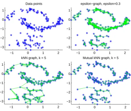
Figure 3: Different similarity graphs, see text for details.
three clusters: two “moons” and a Gaussian. The density of the bottom moon is chosen to be larger than the one of the top moon. The upper left panel in Figure 3 shows a sample drawn from this distribution. The next three panels show the different similarity graphs on this sample.
In the ε-neighborhood graph, we can see that it is difficult to choose a useful parameter ε. With
ε= 0.3 as in the figure, the points on the middle moon are already very tightly connected, while the
points in the Gaussian are barely connected. This problem always occurs if we have data “on different scales”, that is the distances between data points are different in different regions of the space.
Thek-nearest neighbor graph, on the other hand, can connect points “on different scales”. We can
see that points in the low-density Gaussian are connected with points in the high-density moon. This
is a general property ofk-nearest neighbor graphs which can be very useful. We can also see that the
k-nearest neighbor graph can break into several disconnected components if there are high density
re-gions which are reasonably far away from each other. This is the case for the two moons in this example.
The mutualk-nearest neighbor graph has the property that it tends to connect points within regions
of constant density, but does not connect regions of different densities with each other. So the mutual
k-nearest neighbor graph can be considered as being “in between” theε-neighborhood graph and the
k-nearest neighbor graph. It is able to act on different scales, but does not mix those scales with each
other. Hence, the mutualk-nearest neighbor graph seems particularly well-suited if we want to detect
clusters of different densities.
The fully connected graph is very often used in connection with the Gaussian similarity function
s(xi, xj) = exp(−kxi−xjk2/(2σ2)). Here the parameterσplays a similar role as the parameter εin
theε-neighborhood graph. Points in local neighborhoods are connected with relatively high weights,
similarity matrix is not a sparse matrix.
As a general recommendation we suggest to work with thek-nearest neighbor graph as the first choice.
It is simple to work with, results in a sparse adjacency matrix W, and in our experience is less
vulnerable to unsuitable choices of parameters than the other graphs.
The parameters of the similarity graph
Once one has decided for the type of the similarity graph, one has to choose its connectivity parameter
korε, respectively. Unfortunately, barely any theoretical results are known to guide us in this task. In
general, if the similarity graph contains more connected components than the number of clusters we ask the algorithm to detect, then spectral clustering will trivially return connected components as clusters. Unless one is perfectly sure that those connected components are the correct clusters, one should make sure that the similarity graph is connected, or only consists of “few” connected components and very few or no isolated vertices. There are many theoretical results on how connectivity of random graphs
can be achieved, but all those results only hold in the limit for the sample sizen→ ∞. For example,
it is known that forndata points drawn i.i.d. from some underlying density with a connected support
inRd, thek-nearest neighbor graph and the mutualk-nearest neighbor graph will be connected if we
choose k on the order of log(n) (e.g., Brito, Chavez, Quiroz, and Yukich, 1997). Similar arguments
show that the parameterεin theε-neighborhood graph has to be chosen as (log(n)/n)d to guarantee
connectivity in the limit (Penrose, 1999). While being of theoretical interest, all those results do not
really help us for choosingkon a finite sample.
Now let us give some rules of thumb. When working with the k-nearest neighbor graph, then the
connectivity parameter should be chosen such that the resulting graph is connected, or at least has significantly fewer connected components than clusters we want to detect. For small or medium-sized graphs this can be tried out ”by foot”. For very large graphs, a first approximation could be to choose
kin the order of log(n), as suggested by the asymptotic connectivity results.
For the mutualk-nearest neighbor graph, we have to admit that we are a bit lost for rules of thumb.
The advantage of the mutualk-nearest neighbor graph compared to the standard k-nearest neighbor
graph is that it tends not to connect areas of different density. While this can be good if there are clear clusters induced by separate high-density areas, this can hurt in less obvious situations as disconnected parts in the graph will always be chosen to be clusters by spectral clustering. Very generally, one can
observe that the mutualk-nearest neighbor graph has much fewer edges than the standard k-nearest
neighbor graph for the same parameterk. This suggests to chooseksignificantly larger for the mutual
k-nearest neighbor graph than one would do for the standardk-nearest neighbor graph. However, to
take advantage of the property that the mutualk-nearest neighbor graph does not connect regions
of different density, it would be necessary to allow for several “meaningful” disconnected parts of the
graph. Unfortunately, we do not know of any general heuristic to choose the parameterk such that
this can be achieved.
For theε-neighborhood graph, we suggest to chooseεsuch that the resulting graph is safely connected.
To determine the smallest value ofε where the graph is connected is very simple: one has to choose
ε as the length of the longest edge in a minimal spanning tree of the fully connected graph on the
data points. The latter can be determined easily by any minimal spanning tree algorithm. However,
note that when the data contains outliers this heuristic will chooseε so large that even the outliers
are connected to the rest of the data. A similar effect happens when the data contains several tight
clusters which are very far apart from each other. In both cases,εwill be chosen too large to reflect
the scale of the most important part of the data.