Andrew Ang
Columbia University and NBER Geert Bekaert
Columbia University, NBER and CPER
We examine the predictive power of the dividend yields for forecasting excess returns, cash flows, and interest rates. Dividend yields predict excess returns only at short horizons together with the short rate and do not have any long-horizon predictive power. At short horizons, the short rate strongly negatively predicts returns. These results are robust in international data and are not due to lack of power. A present value model that matches the data shows that discount rate and short rate movements play a large role in explaining the variation in dividend yields. Finally, we find that earnings yields significantly predict future cash flows. (JELC12, C51, C52, E49, F30, G12)
In a rational no-bubble model, the price-dividend ratio is the expected value of future cash flows discounted with time-varying discount rates. Because price-dividend ratios, or dividend yields, vary over time, dividend yield variability can be attributed to the variation of expected cash flow growth, expected future risk-free rates, or risk premia. The ‘‘conventional wisdom’’ in the literature (see, among others, Campbell, 1991; Cochrane, 1992) is that aggregate dividend yields strongly predict excess returns, and the predictability is stronger at longer horizons.1Since dividend yields only weakly predict dividend growth, conventional wisdom attributes most of the variation of dividend yields to changing forecasts of expected returns. We critically and comprehensively re-examine this conventional wisdom regarding return predictability on the aggregate market.
We thank Xiaoyan Zhang for help with data. We thank Kobi Boudoukh, Michael Brandt, John Campbell, John Cochrane, George Constantinides, Cam Harvey, Bob Hodrick, Charles Jones, Owen Lamont, Martin Lettau, Jun Liu, Sydney Ludvigson, Chris Neely, Jim Poterba, Tano Santos, Bob Shiller, Tim Simin, Ken Singleton, Rob Stambaugh, Meir Statman, Jim Stock, Ane Tamayo, Samuel Thomson, Ivo Welch, Jeff Wurgler, and seminar participants at Columbia University, Duke University, INSEAD, London Business School, the NY Federal Reserve, NYU, Stanford University, UC San Diego, Wharton, Yale, the American Finance Association, an NBER Asset Pricing meeting, the European Finance Association, and the Western Finance Association for helpful comments. We also thank three anonymous referees and Yacine Aı¨t-Sahalia (the editor) for valuable, extensive comments that greatly improved the article. Andrew Ang thanks the Chazen Institute at Columbia Business School for financial support. Geert Bekaert thanks the NSF for financial support. Address correspondence to Geert Bekaert, Columbia Business school, Room 802, Uris Hall, 3022 Broadway, New York, NY 10027, or e-mail: [email protected].
1
Among those examining the predictive power of the dividend yield on excess stock returns are Fama and French (1988), Campbell and Shiller (1988a,b), Goetzmann and Jorion (1993, 1995), Hodrick (1992), Stambaugh (1999), Wolf (2000), Goyal and Welch (2003, 2004), Engstrom (2003), Valkanov (2003), Lewellen (2004), and Campbell and Yogo (2006).
Our main findings can be summarized as follows. First, the statistical inference at long horizons critically depends on the choice of standard errors. With the standard Hansen–Hodrick (1980) or Newey–West (1987) standard errors, there is some evidence for long horizon predictability, but it disappears when we correct for heteroskedasticity and remove the moving average structure in the error terms induced by summing returns over long horizons (Richardson and Smith 1991, Hodrick 1992, Boudoukh and Richardson, 1993).
Second, we find that the most robust predictive variable for future excess returns is the short rate, but it is significant only at short horizons.2 Whereas, the dividend yield does not univariately predict excess returns, the predictive ability of the dividend yield is considerably enhanced, at short horizons, in a bivariate regression with the short rate. To mitigate data snooping concerns (Lo and MacKinlay 1990, Bossaerts and Hillion 1999, Ferson, Sarkissian, and Simin 2003, Goyal and Welch 2004), we confirm and strengthen this evidence using three other countries: the United Kingdom, France, and Germany.
Third, the dividend yield’s predictive power to forecast future dividend growth is not robust across sample periods or countries. We find that high dividend yields are associated with high future interest rates. While the statistical evidence for interest rate predictability is weak, the same posi-tive relationship is implied by an economic model, and we observe the same patterns across countries.
To help interpret our findings and to deepen our understanding of the data, we provide additional economic analysis. First, we build a nonlinear present value model with stochastic discount rates, short rates, and divi-dend growth, that matches our evidence on excess return predictability. As is true in the data, the model implies that the dividend yield only weakly predicts future cash flows but is positively related to future move-ments in interest rates. While excess discount rates still dominate the variation in price-dividend ratios, accounting for 61%, of the variation short rate movements account for up to 22% of the variation. In compar-ison, dividend growth accounts for around 7% of the variance of price-dividend ratios. The rest of the variation is accounted for by covariance terms.
Because many studies, particularly in the portfolio choice literature, use univariate dividend yield regressions to compute expected returns (Campbell and Viceira, 1999), we use the nonlinear present value model to examine the fit of regression-based expected returns with true expected returns. Consistent with the data, we find that a univariate dividend yield
2
Authors examining the predictability of excess stock returns by the nominal interest rate include Fama and Schwert (1977), Campbell (1987), Breen, Glosten, and Jagannathan (1989), Shiller and Beltratti (1992), and Lee (1992).
regression provides a rather poor proxy to true expected returns. How-ever, using both the short rate and dividend yield considerably improves the fit, especially at short horizons.
Second, using the present value model, we show that long-horizon statistical inference with the standard Hansen–Hodrick (1980) or Newey–West (1987) standard errors is treacherous. We find that both Hansen–Hodrick and Newey–West standard errors lead to severe over-rejections of the null hypothesis of no predictability at long horizons but that standard errors developed by Hodrick (1992) retain the correct size in small samples. The power of Hodrickt-statistics exceeds 0.60 for a 5% test for our longest sample. Moreover, when we pool data across differ-ent countries, the power for our shortest sample increases to 74%. Hence, lack of power is unlikely to explain our results.3
Finally, we focus on expanding the information set to obtain a poten-tially better estimate of true value-relevant cash flows in the future. Dividends may be potentially poor instruments because dividends are often manipulated or smoothed. Bansal and Lundblad (2002) and Bansal and Yaron (2004) argue that dividend growth itself follows an intricate ARMA process. Consequently, it is conceivable that more than one factor drives the dynamics of cash flows. One obvious way to increase the information set is to use earnings. Lamont (1998) argues that the earnings yield has independent forecasting power for excess stock returns in addition to the dividend yield. When we examine the predictive power of the earnings yield for both returns and cash flows, we find only weak evidence for Lamont’s excess return predictability results. However, we detect significant predictability of future cash flows by earnings yields.
This article is organized as follows. Section 1 describes the data. Section 2 contains the main predictability results for returns, while Section 3 discusses cash flow and interest rate predictability by the dividend yield. Section 4 develops a present value model under the null and various alternative models to interpret the empirical results. In Section 5, we conduct a size and power analysis of Hodrick (1992) standard errors. Section 6 investi-gates the predictive power of the earnings yield for excess returns and cash flows. Section 7 concludes and briefly discusses a number of contempora-neous papers on stock return predictability. It appears that the literature is converging to a new consensus, substantially different from the old view. 3
Given the excellent performance of Hodrick (1992) standard errors, we do not rely on the alternative inference techniques that use unit root, or local-to-unity, data generating processes (see, among others, Richardson and Stock 1989, Richardson and Smith 1991, Elliot and Stock 1994, Lewellen 2004, Torous, Valkanov, and Yan 2004, Campbell and Yogo 2006, Polk, Thompson, and Vuolteenaho 2006, Jansson and Moreira 2006). One major advantage of Hodrick standard errors is that the set up can handle multiple regressors, whereas the inference with unit root type processes relies almost exclusively on univariate regressors. The tests for multivariate predictive regressions using local-to-unity data generating processes developed by Polk et al. (2006) involve computationally intensive bootstrapping procedures. This test also has very poor size properties under the nonlinear present value we present in Section 4. These results are available upon request.
1. Data
We work with two data sets, a long data set for the United States, United Kingdom and Germany and a shorter data set for a sample of four countries (United States, United Kingdom, France, and Germany). In the data, dividend and earnings yields are constructed using dividends and earnings summed up over the past year. Monthly or quarterly fre-quency dividends and earnings are impossible to use because they are dominated by seasonal components.
We construct dividend growth and earnings growth from these ratios, producing rates of annual dividend or earnings growth over the course of a month or a quarter. To illustrate this construction, suppose we take the frequency of our data to be quarterly. We denote log dividend growth at a quarterly frequency as gdt,4, with the superscript 4 to denote that it is constructed using dividends summed up over the past year (four quar-ters). We computegtd,4from dividend yieldsD4
t=Pt, where the dividends
are summed over the past year, using the relation
gdt,4¼log D
4
t=Pt
D4
t1=Pt1
Pt
Pt1
, ð1Þ
whereD4
t ¼DtþDt1þDt2þDt3 represents dividends summed over
the past year andPt=Pt1 is the price return over the past quarter.
In our data, the long sample is at a quarterly frequency and the short sample is at a monthly frequency. In the case of the monthly frequency, we append dividend yields, earnings yields, dividend growth and earnings growth with a superscript of 12 to indicate that dividends and earnings have been summed over the past 12 months. We also denote log dividend yields by lower case letters. Hence dy4
t ¼logðD4t=PtÞ, in the case of
quarterly data anddy12
t ¼logðD12t =PtÞ in the case of monthly data. We
also use similar definitions for log earnings yields:ey4
t andey12t .
1.1 Long sample data
Our US data consists of price return (capital gain only), total return (capital gain plus dividend), and dividend and earnings yields on the Standard & Poor’s Composite Index from June 1935 to December 2001. This data is obtained from theSecurity Price Index Record, published by Standard & Poor’s Statistical Service. Lamont (1998) uses the same data set over a shorter period. The long-sample UK data comprises price returns and total returns on the Financial Times (FT) Actuaries Index, and we construct implied dividend yields from these series. For our German data, we take price returns, total returns, and dividend yields on the composite DAX (CDAX) index from the Deutsche Borsche. The long-sample UK and Ge-rman data span June 1953 to December 2001
and were purchased from Global Financial Data. All the long sample data for the United States, United Kingdom, and Germany are at the quarterly frequency, and we consequently use three-month T-bills as quarterly short rates.
Panel A of Table 1 lists summary statistics. US earnings growth is almost as variable as returns, whereas the volatility of dividend growth is less than half the return volatility. The variability of UK and German dividend growth rates is of the same order of magnitude as that of returns. The instruments (short rates, dividend and earnings yields) are all highly persistent. Because the persistence of these instruments plays a crucial role in the finite sample performance of predictability test statis-tics, we report test statistics under the null of a unit root and a stationary process in Panel A. Investigating both null hypotheses is important because unit root tests have very low power to reject the null of a stationary, but persistent, process.
In the United Kingdom and Germany, dividend yields are unambigu-ously stationary, as we reject the null of a unit root and fail to reject the null of stationarity at the 5% level. For the US dividend yield, the evidence for non-stationarity is weak as we fail to reject either hypothesis. This is surprising because the trend toward low dividend yields in the 1990s has received much attention. Figure 1 plots dividend yields for the
Table 1
Sample moments, unit root, and stationarity tests
Excess return
Short rate
Dividend yield
Earnings yield
Dividend growth
Earnings growth
Panel A: Long-sample data
US S&P Data, June 1935–December 2001
Mean 0.0749 0.0409 0.0403 0.0768 0.0532 0.0548 Stdev 0.1684 0.0317 0.0150 0.0297 0.0658 0.1572 Auto 0.1173 0.9548 0.9504 0.9517 0.4071 0.3832 Test statistics
H0: unit root 14.50** 2.194 1.187 1.183 10.83** 10.55**
H0: stationary 0.073 0.635* 0.372 0.336 0.035 0.026
UK FT Data, June 1953–December 2001
Mean 0.0563 0.0751 0.0478 0.0670
Stdev 0.1938 0.0331 0.0131 0.1866
Auto 0.0907 0.9400 0.8290 0.0486
Test statistics
H0: unit root 12.66** 2.559 4.125** 14.64**
H0: stationary 0.037 0.637* 0.199 0.068
Germany DAX Data, June 1953–December 2001
Mean 0.0577 0.0467 0.0287 0.0788
Stdev 0.1921 0.0198 0.0090 0.2086
Auto 0.0851 0.9376 0.9087 0.1136
Test statistics
H0: unit root 12.89** 3.036* 3.336* 12.34**
United States, United Kingdom, and Germany. For the United Kingdom, the dividend yield also declined during the late 1990s, but the United Kingdom experienced similar low level dividend yields during the late 1960s and early 1970s. For Germany, there is absolutely no trend in the dividend yield. If a time trend in dividend yields is a concern for Table 1
(continued)
Excess return
Short rate
Dividend yield
Earnings yield
Dividend growth
Earnings growth Correlations of excess returns, June 1953–December 2001
United States United Kingdom United Kingdom 0.6281
Germany 0.5118 0.4598
Panel B: MSCI data
February 1975–December 2001 United States
Mean 0.0576 0.0745 0.0353 0.0744 0.0529 0.0501 Stdev 0.1513 0.0341 0.0143 0.0305 0.0589 0.0883 Auto 0.0044 0.9675 0.9892 0.9867 0.3187 0.1490 United Kingdom
Mean 0.0604 0.0989 0.0456 0.0874 0.0812 0.0651 Stdev 0.1824 0.0355 0.0123 0.0346 0.0707 0.0973 Auto 0.0184 0.9615 0.9701 0.9758 0.0524 0.2346 France
Mean 0.0542 0.0906 0.0415 0.0675 0.0782 0.0690 Stdev 0.2079 0.0476 0.0188 0.0397 0.0849 0.5868 Auto 0.0745 0.8741 0.9849 0.9627 0.0068 0.0765 Germany
Mean 0.0498 0.0563 0.0359 0.0688 0.0643 0.0564 Stdev 0.1925 0.0241 0.0125 0.0287 0.0876 0.2217 Auto 0.0665 0.9764 0.9860 0.9836 0.0936 0.1781 Correlations of excess returns
United States United Kingdom France United Kingdom 0.5960
France 0.5237 0.5184
Germany 0.4951 0.4742 0.6178
Panel A reports summary statistics of long-sample data for the United States, United Kingdom, and Germany, all at a quarterly frequency. Panel B reports statistics for monthly frequency Morgan Stanley Capital International MSCI data. Excess returns and short rates are continuously compounded. Sample means and standard deviations (Stdev) for excess returns, dividend, and earnings growth have been annualized by multiplying by 4 (12) andpffiffiffiffi4ðpffiffiffiffiffi12Þ, respectively, for the case of quarterly (monthly) frequency data. Short rates for the long-sample (MSCI) data are three-month T-bill returns (one month EURO rates). Dividend and earnings yields, and the corresponding dividend and earnings growth are computed using dividends or earnings summed up over the past year. In Panel A, the unit root test is the Phillips and Perron (1988) test for the estimated regression xt¼þxt1þut under the null xt¼xt1þut. The critical values corresponding top-values of 0.01, 0.025, 0.05, and 0.10 are3:46, 3:14,2:88, and2:57, respectively. The test for stationarity is the Kwiatkowskiet al.(1992) test. The critical values corresponding top-values of 0.01, 0.025, 0.05, and 0.10 are 0.739, 0.574, 0.463, 0.347, respectively.
*p<0.05. **p<0.01.
interpreting the evidence on excess return predictability using the divi-dend yield, international data are clearly helpful. Present value models which impose transversality also imply that dividend yields must be stationary.
Interest rates are also highly persistent variables. While German inter-est rates appear to be stationary, there is some evidence of borderline non-stationary behavior for both US and UK interest rates. Most economic models also imply that interest rates are stationary (Clarida, Galı´, and Gertler, 1999). Our present value model incorporates realistic persistence in short rates, but because of the high persistence of the short rate, we check the robustness of interest rate predictability by using a detrended short rate.
1.2 Short sample MSCI data
The data for the United States, United Kingdom, France, and Germany consist of monthly frequency price indices (capital appreciation only), total return indices (including income), and valuation ratios from Morgan Stanley Capital International (MSCI) in local currency, from February
1940 1950 1960 1970 1980 1990 2000 0
0.02 0.04 0.06 0.08 0.1 0.12
US UK Germany
Figure 1
Dividend yields over the long sample
We plot dividend yields from June 1935 to December 2001 for the United States and from March 1953 to December 2001 for the United Kingdom and Germany.
1975 to December 2001. We use the one-month EURO rate from Data-stream as the short rate.
Panel B of Table 1 shows that the United States has the least variable stock returns with the least variable cash flow growth rates. The extreme variability of French earnings growth rates is primarily due to a few outliers between May 1983 and May 1984, when there are very large movements in price-earnings ratios. Without these outliers, the French earnings growth variability drops to 33%. The variability of short rates, dividend, and earnings yields is similar across countries. The equity pre-mium for the United States, France, Germany, and the United Kingdom roughly lies between 4 and 6% during this sample period. Dividend yields and short rates are again very persistent over the post-1975 sample. We also report excess return correlations showing that correlations range between 0.47 and 0.60. The correlations for the United States, United Kingdom, and Germany are similar to the correlations over the post-1953 period reported in Panel A.
2. The Predictability of Equity Returns
2.1 Predictability regressions
Denote the gross return on equity by Ytþ1¼ ðPtþ1þDtþ1Þ=Pt and the
continuously compounded return byytþ1¼logðYtþ1Þ. The main
regres-sion we consider is
~
ytþk¼kþkztþ"tþk,k, ð2Þ
where ~ytþk¼ ð =kÞ½ðytþ1rtÞ þ:::þ ðytþkrtþk1Þ is the annualized k-period excess return for the aggregate stock market,rt is the risk-free
rate from t to tþ1, and ytþ1rt is the excess one period return from
timettotþ1. A period is either a monthð ¼12Þor a quarterð ¼4Þ. All returns are continuously compounded. The error term"tþk,kfollows a
MAðk1Þ process under the null of no predictabilityðk¼0Þbecause
of overlapping observations. We use log dividend yields and annualized continuously compounder risk-free rates as instruments inzt.
We estimate the regression (2) by OLS and compute standard errors of the parameters¼ ð
kÞ
following Hodrick (1992). Using generalized method of moments, (GMM)has an asymptotic distributionpffiffiffiffiTð^Þ a
Nð0,Þwhere¼Z01S0Z01,Z0¼EðxtxtÞ, andxt ¼ ð1 ztÞ
. Hodrick exploits covariance stationarity to remove the overlapping nature of the error terms in the standard error computation. Instead of summing"tþk,k
into the future to obtain an estimate ofS0, Hodrick sumsxtxtjinto the
^
S0¼ 1
T XT
t¼k
wktwkt, ð3Þ
where
wkt¼"tþ1,1 Xk1
i¼0 xti
!
:
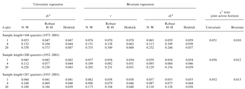
We show in section 5 that the performance of Hodrick (1992) standard errors is far superior to the Newey–West (1987) standard errors or the robust GMM generalization of Hansen and Hodrick (1980) standard errors (see Appendix A) typically run in the literature. Hence, our pre-dictability evidence exclusively focuses on Hodrickt-statistics. Mindful of Richardson’s (1993) critique of focusing predictability tests on only one particular horizonk, we also compute joint tests across horizons. For the quarterly (monthly) frequency data, we test for predictability jointly across horizons of 1, 4, and 20 quarters (1, 12, and 60 months). Appendix B details the construction of joint tests across horizons accommodating Hodrick standard errors. Finally, when considering predictability in multiple countries, we estimate pooled coefficients across countries and provide joint tests of the null of no predictability. Pooled estimations mitigate the data-mining problem plaguing US data and, under the null of no predictability, enhance efficiency because the correlations of returns across countries are not very high (Table 1). Appendix C details the econometrics underlying the pooled estimations.
2.2 Return predictability in the United States
We report results for several sample periods, in addition to the full sample 1935–2001. Interest rate data are hard to interpret before the 1951 Treasury Accord, as the Federal Reserve pegged interest rates during the 1930s and the 1940s. Hence, we examine the post-Accord period, starting in 1952. Second, the majority of studies establishing strong evidence of predictabil-ity use data before or up to the early 1990s. Studies by Lettau and Ludvigson (2001) and Goyal and Welch (2003) point out that predictability by the dividend yield is not robust to the addition of the 1990s decade. Hence, we separately consider the effect of adding the 1990s to the sample. We start by focusing on a univariate regression with the dividend yield as the regressor. Figure 2 shows the slope coefficients for three different sample periods, using the quarterly US S&P data. The left-hand column reports the dividend yield coefficients, whereas the right-hand column reports t-statistics computed using Newey–West (1987), robust Hansen–Hodrick (1980), and Hodrick (1992) standard errors. For the
Newey–West errors, we usekþ1 lags. The coefficient pattern is similar across the three periods, but the coefficients are twice as large for the period omitting the 1990s from the sample. For the other two periods (1935–2001 and 1952–2001), the one-period coefficient is about 0.110,
1935-2001 Dividend Yield Coefficient 1935-2001 T-statistic
0 2 4 6 8 10 12 14 16 18 20 0.08 0.085 0.09 0.095 0.1 0.105 0.11 0.115 Horizon (quarters) t n ei ciff e o C
0 2 4 6 8 10 12 14 16 18 20 0 0.5 1 1.5 2 2.5 3 3.5 4 4.5 5 5.5 Horizon (quarters) t at s − T Robust Hansen−Hodrick Hodrick Newey−West
1952-2001 Dividend Yield Coefficient 1952-2001 T-statistic
0 2 4 6 8 10 12 14 16 18 20 0.04 0.05 0.06 0.07 0.08 0.09 0.1 0.11 0.12 Horizon (quarters) t n ei cif f e o C
0 2 4 6 8 10 12 14 16 18 20 0 0.5 1 1.5 2 2.5 3 3.5 4 4.5 5 5.5 Horizon (quarters) t at s − T Robust Hansen−Hodrick Hodrick Newey−West
1935-1990 Dividend Yield Coefficient 1935-1990 T-statistic
0 2 4 6 8 10 12 14 16 18 20 0.16 0.17 0.18 0.19 0.2 0.21 0.22 0.23 0.24 0.25 Horizon (quarters) t n ei ciff e o C
0 2 4 6 8 10 12 14 16 18 20 0 0.5 1 1.5 2 2.5 3 3.5 4 4.5 5 5.5 Horizon (quarters) t at s − T Robust Hansen−Hodrick Hodrick Newey−West Figure 2
Dividend yield coefficients andt-statistics from US regressions
The left (right) column shows the dividend yield coefficients k (t-statistics) in the regression ~
ytþk¼þkdy4tþ"tþk,k, where~ytþkis the cumulated and annualizedk-quarter ahead excess return
anddy4
t is the log dividend yield.T-statistics are computed using Robust Hansen-Hodrick (1980),
rises until the one-year horizon, and then decreases, before increasing again near 20 quarters.
Over 1935–2001, the Hodrickt-statistic is above 2 only for horizons 2– 4 quarters. However, there is no evidence of short-run predictability (at the one-quarter horizon) or long-horizon predictability. We draw a very different picture of predictability if we use Newey–West or robust Hansen–Hodrick t-statistics, which are almost uniformly higher than Hodrickt-statistics. Using Newey–West standard errors, the evidence in favor of predictability would extend to eight quarters for the full sample. Over the 1952–2001 sample, there is no evidence of predictability, whereas for the 1935–1990 period, the evidence for predictability is very strong, whatever the horizon, with all threet-statistics being above 2.4.
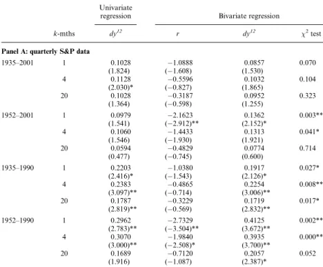
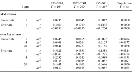
Table 2 summarizes the excess return predictability results for horizons of one month (quarter), one year, and five years. We only report
t-statistics using Hodrick standard errors. In addition to the sample periods shown in Figure 2, we also show the 1952–1990 period, which is close to the 1947–1994 sample period in Lamont (1998). When we omit the 1990s, we confirm the standard results found by Campbell and Shiller (1988a,b) and others: the dividend yield is a significant predictor of excess
Table 2
Predictability of US excess returns
Univariate
regression Bivariate regression
k-mths dy12
r dy12 2
test
Panel A: quarterly S&P data
1935–2001 1 0.1028 1.0888 0.0857 0.070
(1.824) (1.608) (1.530)
4 0.1128 0.5596 0.1032 0.104
(2.030)* (0.827) (1.865)
20 0.1028 0.3187 0.0952 0.323
(1.364) (0.598) (1.255)
1952–2001 1 0.0979 2.1623 0.1362 0.003**
(1.541) (2.912)** (2.152)*
4 0.1060 1.4433 0.1313 0.041*
(1.546) (1.930) (1.921)
20 0.0594 0.4829 0.0774 0.714
(0.477) (0.745) (0.600)
1935–1990 1 0.2203 1.0380 0.1917 0.027*
(2.416)* (1.543) (2.126)*
4 0.2383 0.4865 0.2254 0.008**
(3.097)** (0.714) (3.006)**
20 0.1787 0.3229 0.1719 0.017*
(2.819)** (0.569) (2.832)**
1952–1990 1 0.2962 2.7329 0.4125 0.002**
(2.783)** (3.504)** (3.672)**
4 0.3070 1.9840 0.3935 0.000**
(3.000)** (2.508)* (3.700)**
20 0.1689 0.7120 0.2057 0.052
returns at all horizons. However, when we use all the data, we only find 5% significance at the one-year horizon for the longest sample. A test for predictability by the dividend yield jointly across horizons rejects with a
p-value of 0.014 for the 1935–1990 period, but fails to reject with a
p-value of 0.587 over the whole sample, even though the shorter horizon
t-statistics all exceed 1.5 in absolute value. While it is tempting to blame the bull market of the 1990s for the results, our data extend until the end of 2001 and hence incorporate a part of the bear market that followed. For the 1975–2001 sample, reported in Panel B, the dividend yield also fails to predict excess returns.
Table 2 also reports bivariate regression results with the short rate as an additional regressor. For the post-Treasury Accord 1952–2001 sample, a 1% increase in the annualized short rate decreases the equity premium by about 2.16%. The effect is significant at the 1% level. A joint test on the interest rate coefficients across horizons rejects strongly for both the 1952–2001 period ðp-value¼0:004Þ and the 1952–1990 period
ðp-value¼0:000Þ. The predictive power of the short rate dissipates quickly for longer horizons but remains borderline significant at the 5% level at the one-year horizon.4If expected excess returns are related only to short rates and short rates follow a univariate autoregressive process, the persistence of the interest rate (0.955 in Table 1) implies that the coefficient on the short rate should tend to zero slowly for long horizons. In fact, the decay rate should be 1=k ð1kÞ=ð1Þfor horizonk. The
Table 2 (continued)
Univariate
regression Bivariate regression
k-mths dy12
r dy12 2
test
Panel B: monthly MSCI data
1975–2001 1 0.0274 2.4358 0.1364 0.057
(0.405) (2.388)* (1.626)
12 0.0106 1.2470 0.0669 0.395
(0.141) (1.361) (0.744)
60 0.0884 0.3451 0.1207 0.857
(0.475) (0.238) (0.397)
We estimate regressions of the form~ytþk¼kþztþtþk,kwhere~ytþkis the cumulated and annualized k-period ahead excess return, with instrumentszt being log dividend yields or risk-free rates and log
dividend yields together.T-statistics in parentheses are computed using Hodrick (1992) standard errors. For Panel A (B), horizonskare quarterly (monthly). The2test column reports ap-value for a test that
both the risk-free rate and log dividend yield coefficients are jointly equal to zero. *p<0.05.
**p<0.01.
4
The results do not change when a detrended short rate is used instead of the level of the short rate or when we use a dummy variable over the period from October 1979 to October 1982 to account for the monetary targeting period.
decay rate in data is clearly more rapid, indicating that either expected excess returns or risk-free rates, or both, are multifactor processes.
In the bivariate regression, the dividend yield coefficient is only signifi-cant at the 5% level for the one-quarter horizon. Joint tests reject at the 1% (5%) level for the one-quarter (four-quarter) horizon but fail to reject at long horizons. When we omit the 1990s, the predictive power of the short rate becomes even stronger. A joint predictability test still fails to reject the null of no predictability at long horizons, but the p-value is borderline significant (0.052). Over the 1975–2001 sample, the coefficient on the short rate remains remarkably robust and is significant at the 5% level. While the coefficient on the dividend yield is no longer significantly different from zero, it is similar in magnitude to the full sample coefficient and a joint test is borderline significant ðp-value¼0:057Þ. The Richardson (1993) joint predictability test over all horizons and both predictors rejects at the 1% level in the samples excluding the 1990s and the full sample, rejects at the 5% level for 1952–2001, and rejects at the 10% level for 1975–2001.
Looking at the 1951–2001 and 1975–2001 samples, the evidence for the bivariate regression at short horizons is remarkably consistent. Moreover, the coefficient on the dividend yield is larger in the bivariate regression than in the univariate regression. This suggests that the univariate regres-sion suffers from an omitted variable bias that lowers the marginal impact of dividend yields on expected excess returns. Engstrom (2003), Menzly, Santos, and Veronesi (2004), and Lettau and Ludvigson (2005) also note that a univariate dividend yield regression may understate the dividend yield’s ability to forecast returns.
2.3 Predictability of excess returns in four countries
The weak predictive power of the univariate dividend yield in the full sample may simply be a small sample phenomenon due to the very special nature of the last decade for the US stock market. Alternatively, the conventional wisdom of strong long-horizon excess return predictability by dividend yields before 1990 may be a statistical fluke. International evidence can help us to sort out these two interpretations of the data and check the robustness of predictability patterns observed in US data.
Figure 3 displays the univariate dividend yield coefficients and their
t-statistics using Hodrick standard errors in the 1975–2001 sample. First, none of the patterns in other countries resembles the US pattern. For France and Germany, and to a lesser degree for the United Kingdom, the coefficients first increase with horizon, then decrease, and finally increase again. This is roughly the pattern we see in US data for the longer samples. However, for France and Germany, the coefficients are small at short horizons and are negative for many horizons. They are also never statistically significant. The UK coefficient is larger and remains positive across horizons: it is also significantly different from zero at the
very shortest horizons. These results are opposite to the results in a recent study by Campbell (2003), who reports strong long-horizon predictability for France, Germany, and the United Kingdom over similar sample periods. We find that Campbell’s conclusions derive from the use of Newey–West (1987) standard errors, and the predictability disappears when Hodrick (1992) standard errors are employed.
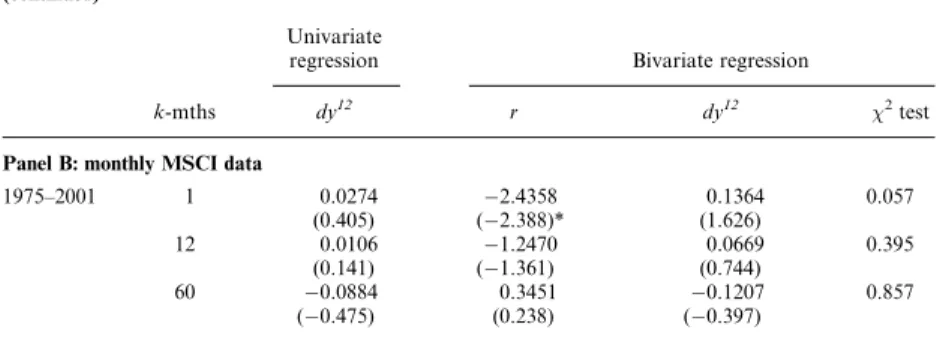
For the United Kingdom and Germany, we also investigate the longer 1953–2001 sample in Panel A of Table 3. The first column reports the univariate dividend yield coefficients. We only find significance at the one-year horizon for the UK, but the coefficients are all positive and more than twice as large as the US coefficients.5Germany’s dividend yield
5
For the United Kingdom, we also looked at a sample spanning 1935–2001, where we find a significant univariate dividend yield coefficient at the five-year horizon but not at the one-quarter horizon.
−0.1 −0.05 0 0.05 0.1
US dy coefficient
0.1 0.15 0.2 0.25 0.3
0.35 UK dy coefficient
−0.02 0 0.02 0.04
0.06 FR dy coefficient
0 10 20 30 40 50 60 −0.04
−0.02 0 0.02 0.04
GR dy coefficient
Horizon (months)
−1 0 1 2
US t−stat
−1 0 1 2
UK t−stat
−1 0 1 2
FR t−stat
0 10 20 30 40 50 60 −1
0 1 2
GR t−stat
Horizon (months)
Figure 3
Dividend yield coefficients andt-statistics in four countries
The left (right) column shows the dividend yield coefficients k (t-statistics) in the regression ~
ytþk¼þkdy12t þ"tþk,k, where~ytþkis the cumulated and annualizedk-month ahead excess return
anddy12
t is the log dividend yield.T-statistics are computed using Hodrick (1992) standard errors. The
coefficients are the same order of magnitude than those of the United States, but are all insignificant.
Figure 4 displays the coefficient patterns for the annualized short rate and its associatedt-statistics in the bivariate regression for the 1975–2001 sample. Strikingly, this coefficient pattern is very robust across countries. For all countries, the one-month coefficient is negative, below 3 for Table 3
Excess return regressions across countries
Univariate
regression Bivariate regression
k-qtrs dy4only J-test r dy4 2Test J-test
Panel A: quarterly long-sample data
United Kingdom, 1953–2001 1 0.2280 1.2148 0.2596 0.069 (1.449) (1.500) (1.675)
4 0.2600 0.7138 0.2777 0.041* (2.075)* (0.896) (2.273)* 20 0.1290 0.1075 0.1264 0.326
(1.403) (0.182) (1.338)
Germany, 1953–2001 1 0.0740 3.4079 0.1083 0.030* (0.827) (2.545)* (1.204)
4 0.1235 2.1027 0.1443 0.094 (1.366) (1.679) (1.610) 20 0.0415 0.4758 0.0372 0.814
(0.397) (0.489) (0.360) Pooled United States,
United Kingdom,
1 0.1230 (1.964)*
0.496 1.958 (2.927)**
0.1600 (2.626)**
0.001** 0.133 Germany, 1953–2001 4 0.1523 0.344 1.2561 0.1754 0.008** 0.307
(2.268)* (1.909) (2.709)**
20 0.0657 0.495 0.0157 0.0653 0.637 0.658 (0.763) (0.0319) (0.818)
Univariate
regression Bivariate regression
k-mths dy12
only J-test r dy12
chi2test J-test Panel B: monthly MSCI data
Pooled United States, United Kingdom, Germany,
1 0.0560 (0.866)
0.096 1.8161 (2.718)**
0.1640 (2.222)*
0.031* 0.016* France, 1975–2001 12 0.0386 0.327 1.1392 0.1060 0.229 0.113
(0.533) (2.045)* (1.337) 60 0.0169
(0.130)
0.663 0.1799 (0.405)
0.0035 (0.033)
0.699 0.887 We estimate regressions of the form~ytþk¼kþztþ"tþk,kwhere~ytþkis the cumulated and annualized k-period ahead excess return, with instrumentsztbeing log dividend yields or risk-free rates and log
dividend yields together. T-statistics in parentheses are computed using Hodrick (1992) standard errors. Panel A estimates the regression pooling data across the United States, United Kingdom, and Germany on data from 1953–2001. The estimates listed in the United Kingdom and Germany panels allow each country to have its own predictive coefficients and intercepts, but we compute Seemingly Unrelated Regression (SUR) standard errors following the method outlined in the Appendix. The coefficients listed in the pooled panel are produced by constraining the predictive coefficients to be the same across countries. In Panel B, monthly frequency MSCI data is used from 1975–2001. The column labeled ‘‘2
test’’ reports ap-value for a test that both the risk-free rate and log dividend yield coefficients are jointly equal to zero. The ‘‘J-test’’ columns reportp-values for a2test of the overidentifying restrictions.
*p<0.05. **p<0.01.
Germany and around 1:5 for France. The coefficient monotonically increases with the horizon, leveling off around 0.35 for the United States, 0.13 for France, 1.41 for Germany, and0:74 for the United Kingdom. The t-statistics are larger in absolute magnitude for short horizons. In particular, at the one-month horizon, the short rate coefficients are statistically different from zero for the United States and Germany and thet-statistics are near 1.5 (in absolute value) for the United Kingdom and France.
Panel A of Table 3 reports the bivariate coefficients for the long sample for the United Kingdom and Germany. Both countries have negative coefficients on the short rate. For Germany, the short rate coefficient is highly significant, while the UKt-statistic is only 1:5. For both coun-tries, the short rate coefficients increase with horizon and turn positive at
−3 −2 −1 0
1 US rf coefficient
−2.5 −2 −1.5 −1 −0.5
UK rf coefficient
−2 −1.5 −1 −0.5 0
0.5 FR rf coefficient
0 10 20 30 40 50 60 −4
−2 0
2 GR rf coefficient
Horizon (months)
−3 −2 −1 0 1
2 US t−stat
−3 −2 −1 0 1 2
UK t−stat
−3 −2 −1 0 1
2 FR t−stat
0 10 20 30 40 50 60 −3
−2 −1 0 1
2 GR t−stat
Horizon (months)
Figure 4
Short rate coefficients from bivariate regressions in four countries
The left (right) column shows the risk-free rate coefficientsk(t-statistics) from the bivariate regression ~
ytþk¼þztkþ"tþk,k, where~ytþkis the cumulated and annualizedk-month ahead excess return and zt¼ ðrtdy12t Þcontains the annualized risk-free rate and the log dividend yield. We report only the short
rate coefficient.T-statistics are computed using Hodrick (1992) standard errors. The monthly data is from MSCI and the sample period is from 1975 to 2001.
the five-year horizon. Similar to the United States, the dividend yield coefficients are larger in the bivariate regressions than in the univariate regression. However, the dividend yield coefficient is still only signifi-cantly different from zero at the 5% level in the United Kingdom at the one-year horizon.
To obtain more clear-cut conclusions, Table 3 reports pooled predict-ability coefficients and tests. We pool across the United States, United Kingdom, and Germany for the long sample in Panel A, and pool across all four countries in Panel B. The univariate dividend yield regression delivers mixed evidence across the two samples. For the long sample, the dividend yield coefficients are larger than 0.10 at the quarter and one-year horizons and statistically significant at the 5% level. The joint pre-dictability tests for the shorter sample reveal a pattern of small dividend yield coefficients that decrease with horizon and are never significantly different from zero. We also report aJ-test of the overidentifying restric-tions for the joint estimation (see Appendix C). This test fails to reject for all horizons in both the long and short samples, which suggests that pooling is appropriate.
What is most striking about the bivariate regression results across the long and short samples is the consistency of the results. At the one-period forecasting horizon, the short rate coefficient is1:96 in the long sample and 1:82 in the short sample, both significant at the 1% level. The bivariate regression also produces a dividend yield coefficient around 0.16 that is significant at the 1% (5%) level in the long (short) sample. Not surprisingly, the joint test rejects at the 5% level. However, for the short sample, the test of the overidentifying restrictions rejects at the 5% level, suggesting that pooling may not be appropriate for this horizon. For longer horizons, this test does not reject, and the evidence for predictability weakens. Nevertheless, for the long sample, we still reject the null of no predictability at the 1% level for the one-year horizon.
We conclude that whereas the dividend yield is a poor predictor of future returns in univariate regressions, there is strong evidence of pre-dictability at short horizons using both dividend yields and short rates as instruments. The short rate is the stronger predictor and predicts excess returns with a coefficient that is negative in all four countries that we consider.
3. Do Dividend Yields Predict Cash flows or Interest Rates?
Our predictability results overturn some conventional, well-accepted results regarding the predictive power of dividend yields for stock returns. The dividend yield is nonetheless a natural predictor for stock returns. Define the discount rate t as the log conditional expected total return,
expð tÞ ¼Et½ðPtþ1þDtþ1Þ=Pt Et½Ytþ1: ð4Þ
Denotinggd
tþ1as log dividend growth,gtdþ1¼logðDtþ1=DtÞ, we can
rear-range (4) and iterate forward to obtain the present value relation:
Pt
Dt
¼Et
X1
i¼1
exp X
i1
j¼0
tþjþ
Xi j¼1
gdtþj !
" #
, ð5Þ
assuming a transversality condition holds. Note that Equation (5) is different from the Campbell and Shiller (1988a,b) log linear approxima-tion for the log price-dividend ratioptdt¼logðPt=DtÞ:
ptdtcþEt
X1
j¼1
j1ðytþjgtdþjÞ
" #
, ð6Þ
where c and are linearization constants. Equation (5) is an exact expression and involves true expected returns. In contrast, the approx-imation in Equation (6) involves actual total log returnsyt.
Since the price-dividend ratio varies through time, so must some com-ponent on the RHS of Equation (5). As the discount rate is the sum of the risk-free rate and a risk premium, time-varying price-dividend ratios or dividend yields consequently imply that either risk-free rates, risk pre-miums, or cash flows must be predictable by the dividend yield. Although we find predictable components in excess returns, the dividend yield appears to be a strong predictive instrument at short horizons only when augmented with the short rate. Of course, the nonlinearity in Equation (5) may make it difficult for linear predictive regressions to capture these predictable components. In this section, we examine whether the dividend yield predicts cash flow growth rates or future interest rates.6
3.1 Dividend growth predictability
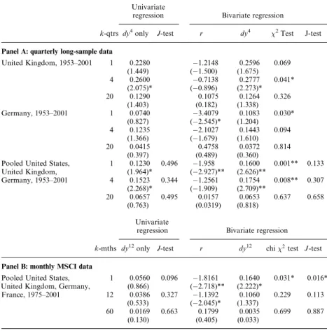
Panel A of Table 4 investigates US dividend growth over two samples, 1935–2001 and 1952–2001. Over the longer sample, we find no evidence of dividend growth predictability. For the shorter sample, high dividend yields predict future high dividend growth at the one- and four-quarter 6
Goyal and Welch (2003) show that in a Campbell and Shiller (1988a,b) log-linear framework, the predictive coefficient on the log dividend yield in a regression of the one-period total return on a constant and the log dividend yield can be decomposed into an autocorrelation coefficient of the dividend yield and a coefficient reflecting the predictive power of dividend yields for future cash-flows. In Section 4, we attribute the time variation of the dividend yield into its three possible components—risk-free rates, excess returns, and cash flows—using a nonlinear present value model.
horizons. The magnitude of the coefficients is preserved in the bivariate regression, but the coefficient is no longer significantly different from zero at the one-quarter horizon and borderline significant at the one-year horizon. However, the short rate coefficient is positive and strongly significant at the one-quarter horizon. The coefficient becomes smaller and insignificant at longer horizons. The joint tests (across the two Table 4
Predictability of dividend growth
Univariate
regression Bivariate regression
k-qtrs dy4only r dy4 2test
Panel A: US S&P data
1935–2001 1 0.0036 0.0586 0.0027 0.974
(0.175) (0.227) (0.147)
4 0.0126 0.0389 0.0133 0.738
(0.504) (0.157) (0.588)
20 0.0100 0.0384 0.0091 0.886
(0.489) (0.299) (0.483)
1952–2001 1 0.0251 0.3541 0.0188 0.000**
(2.476)* (2.191)* (1.599)
4 0.0259 0.1791 0.0228 0.005**
(2.503)* (1.131) (1.903)
20 0.0165 0.0863 0.0132 0.325
(0.927) (0.808) (0.649)
Panel B: pooled across the United States, United Kingdom, and Germany
1953–2001 1 0.1545 0.6991 0.1677 0.000**
(15.54)** (4.296)** (14.16)**
4 0.1552 0.4897 0.1642 0.000**
(14.64)** (3.005)** (13.19)**
20 0.0489 0.2678 0.0555 0.030*
(2.544)* (2.276) (2.452)* Univariate
regression Bivariate regression
k-mths dy12only r dy12 2test
Panel C: pooled across United States, United Kingdom, Germany, and France
1975–2001 1 0.0179 0.3248 0.0371 0.616
(0.757) (1.194) (1.286)
12 0.0116 0.3348 0.0082 0.377
(0.440) (1.511) (0.281)
60 0.0077 0.0702 0.0025 0.266
(0.138) (0.359) (0.059)
We estimate regressions of cumulated and annualizedk-period ahead dividend growth, on log dividend yields alone or risk-free rates and log dividend yields together. Panels B and C pool data jointly across countries, constraining the predictive coefficients to be the same across countries. The2test column
reports ap-value for a test that both the risk-free rate and log dividend yield coefficients are jointly equal to zero.T-statistics in parentheses are computed using Hodrick (1992) standard errors.
*p<0.05. **p<0.01.
coefficients) reject at the 1% level for both the one- and four-quarter horizons.
Campbell and Shiller (1988a,b) note that the approximate linear relation (6) implies a link between high dividend yields today and either high future returns, or low future cash flows, or both. Hence, the positive sign of the dividend yield coefficient in the short sample is surprising. However, the Campbell–Shiller intuition is incomplete because it relies on a linear approximation to the true present value relation (5). Positive dividend yield coefficients in predictive cash-flow regressions can arise in rational models. For example, Ang and Liu (2006) show how the nonlinearity of the present value model can induce a positive dividend yield coefficient. Menzly, Santos, and Veronesi (2004) show that the dividend yield coeffi-cient is a function of a variable capturing shocks to aggregate preferences. Consequently, it changes over time and can take positive values.
In Panels B and C of Table 4, we investigate the relation between dividend yields and cash-flows for other countries. Panel B pools data across the United States, United Kingdom, and Germany for the 1953– 2001 sample. Unlike the US post-1952 sample, the dividend yield coeffi-cients are strongly negative. Because the United Kingdom and German coefficients are so different from the United States (data not shown), a pooled result is hard to interpret, and the GMM over-identifying restric-tions are strongly rejected with ap-value of less than 0.001. Nevertheless, pooling yields negative, not positive, dividend yield coefficients. The short rate coefficients are strongly positive and are about twice the magnitude of the US coefficients (a 1% increase in the short rate approxi-mately forecasts an annualized 70 basis point increase in expected divi-dend growth over the next quarter).
Panel C reports coefficients for the MSCI sample. The dividend yield coefficients are small, mostly negative and never statistically significantly different from zero. The short rate coefficients are also insignificant, although they are similar in magnitude to the coefficient found in long-term US data. There is no general pattern in the individual country dividend yield coefficients (data not shown): the dividend yield coefficient in the univariate regression is positive (negative) in the United States and United Kingdom (France and Germany), with the dividend yield coeffi-cients retaining the same signs in the bivariate regression in each country. All in all, we conclude that the evidence for linear cash-flow predictability by the dividend yield is weak and not robust across countries or sample periods.7
7
It is conceivable that dividend yields exhibit stronger predictive power forrealdividend growth. However, we find the results for real and nominal growth to be quite similar. In the long US sample, the dividend yield fails to forecast future ex-post real dividend growth and the coefficients are positive. For the shorter sample, pooled results across the four countries produce negative coefficients that are actually significant at short horizons. These results are available upon request. Campbell (2003) also finds analogous results.
3.2 Interest Rate Predictability
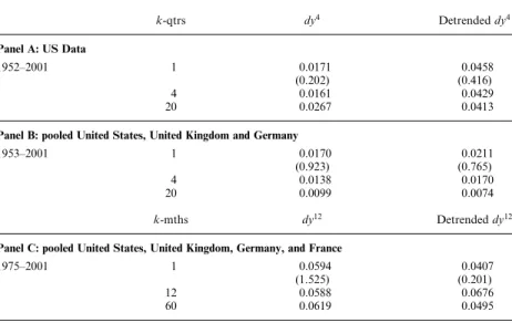
We examine the possibility that the dividend yield predicts risk-free rates in Table 5, which reports coefficients of a regression of future annualized cumulated interest rates on log dividend yields. The persistence of the risk-free rate causes two econometric problems in linear regressions. First, because the interest rate and dividend yield are both persistent variables, the regression is potentially subject to spurious regression bias. To address this issue, we also report results using the detrended dividend yield, which is the dividend yield relative to a 12-month moving average (Campbell 1991, Hodrick 1992). Second, the residuals in the predictive regression are highly autocorrelated, which means that the use of Hodrick (1992) standard errors is inappropriate. For a one-period horizon, we use Cochrane–Orcutt standard errors and generalize the use of this procedure to panel data in the Appendix. We do not report standard errors for horizons greater than one period, because the residuals contain both autocorrelation and moving average effects that cannot be accommo-dated in a simple procedure.
Table 5 reports that the long sample for the United States shows a positive effect of the dividend yield on future interest rates. The effect is economically small (a 1% increase in the log dividend yield predicts an increase in the one-quarter short rate by 1.7 basis points on an annualized
Table 5
Predictability of risk-free rates
k-qtrs dy4 Detrendeddy4
Panel A: US Data
1952–2001 1 0.0171 0.0458
(0.202) (0.416)
4 0.0161 0.0429
20 0.0267 0.0413
Panel B: pooled United States, United Kingdom and Germany
1953–2001 1 0.0170 0.0211
(0.923) (0.765)
4 0.0138 0.0170
20 0.0099 0.0074
k-mths dy12 Detrendeddy12
Panel C: pooled United States, United Kingdom, Germany, and France
1975–2001 1 0.0594 0.0407
(1.525) (0.201)
12 0.0588 0.0676
60 0.0619 0.0495
We estimate regressions of cumulated and annualizedk-period ahead average risk-free rates by log dividend yields. The detrended log dividend yield refers to the difference between the log dividend yield and a moving average of log dividend yields over the past year. Panel c pools data across countries. We compute Cochrane-Orcuttt-statistics (in parentheses) for a one-quarter horizon.
basis next quarter). Using a detrended dividend yield also leads to the same positive sign. While both effects are statistically insignificant, we view the relationship between dividend yields and future interest rates as economically important because interest rates are a crucial component of a present value relation. From the present value relation (5), we expect a positive relation between dividend yields and future discount rates. The interest rate enters the discount rate in two ways. The discount rate is the sum of the risk-free rate and the risk premium and enters these two components with opposite signs. It is the first component that gives rise to the positive relation.
Although not statistically significant, the positive sign of interest rate predictability by dividend yields is robust. First, omitting the 1990s does not change the inference, but actually increases thet-statistics. Second, we also find a positive sign for Germany and the United Kingdom in the long sample and for all countries in the short sample. In particular, for MSCI data, the individual coefficients range from 0.036 in the United States to 0.085 in France at the one-month horizon.8
4. A Present Value Model for Stock Returns
In this section, we present a present value model to shed light on what kind of discount rate processes are most consistent with the predictability evidence.
4.1 The model
We start with the basic present value relation in (5) and parameterize the dynamics of the discount rates and cash flows. We assume that the continuously compounded risk-free rate rt and log dividend growth gtd
follow the VAR:
Xt¼þXt1þ"t, ð7Þ
where Xt ¼ ðrt,gdtÞ
and "t IIDNð0,Þ. Let the discount rate, t, in
Equation (4) follow the process:
t¼þXtþ t1þut, ð8Þ
with utIIDNð0,2Þ and "t and ut are independent. We denote the
individual components of as¼ ðr,gdÞ.
8
We also examine the predictive power of the dividend yield for ex-post real interest rates, similar to Campbell (2003). Although the individual coefficients across countries fail to have a consistent sign, pooled results produce positive coefficients at all horizons, as in the nominal case. However, the coefficients are not statistically significant.
Proposition 4.1. Assuming that Xt¼ ðrt,gdtÞ
follows Equation (7) and that the log conditional total expected return t follows (8), the
price-dividend ratio Pt=Dt is given by
Pt
Dt
¼X
1
i¼1
expðaiþbiXtþci tÞ, ð9Þ
where
aiþ1¼ aiþciþ
1 2c
2
i
2þ ðe
2þbiþciÞ
þ1
2ðe2þbiþciÞ
ð
e2þbiþciÞ
biþ1¼ ðe2þbiþciÞ
ciþ1¼ci1,
ð10Þ
where e2¼ ð0, 1Þ,aiand ciare scalars, and biis a21vector. The initial
conditions are given by
a1¼e2þ1
2e
2e2 b1¼e2
c1¼ 1:
ð11Þ
Proof: See Appendix D.
Proposition 4.1 implies that the dividend yield is a highly nonlinear function of interest rates, excess returns, and cash flows. Not surprisingly, if discount rates are persistent, thecicoefficients are negative and higher
discount rates decrease the price-dividend ratio. Analogously, when divi-dend growth is positively autocorrelated, a positive shock to dividivi-dend growth likely increases the price-dividend ratio, unless it entails an oppo-site discount rate effectðdg >0Þ.
The present value model endogenously generates heteroskedasticity. While previous studies model returns and dividend yields in finite-order VAR systems (see, among many others, Hodrick 1992, Campbell and Shiller 1988a,b, Stambaugh 1999), a VAR cannot fully capture the non-linear dynamics of dividend yields implied by the present value model. We can also contrast our present value model with Goetzmann and Jorion (1993, 1995) and Bollerslev and Hodrick (1996), who either ignore the cointegrating relation between dividends and price levels that
characterizes rational pricing or only develop approximate solutions. In contrast, we impose cointegration between dividends and prices and our solution is exact.
Under the special case of constant total returns, that is t ¼, with
¼¼2¼0, and IID dividend growthðgd
t ¼d þd"gtÞ, Equation (9)
simplifies to a version of the Gordon model:
Pt
Dt
¼ expðd þ
1 2
2
dÞ
1expðdþ122dÞ
:
Another important special case of the model is constant expected excess returns, where t ¼þrt, so¼ ð1, 0Þ, and¼2¼0. In this case, the
time variation in total expected returns is all due to the time variation in interest rates. This is the relevant null model for our excess return regressions where the expected excess return is constant but the total expected return varies with the interest rate.
Under the null of constant expected excess returns, the gross total returnYt¼ ðPtþ1þDtþ1Þ=PtÞless the gross interest rate expðrtÞis
Et½Ytþ1expðrtÞ ¼expðrtÞ½expðÞ 1,
so regressing the simple net excess return on the interest rate actually yields a nonzero coefficient onrt. The scaled expected return, Et½Ytþ1=expðrtÞ is
constant and equal to. The predictability regressions typically run in the literature do not correspond to any of these two concepts, since they use log returns ~ytþ1logðYtþ1Þ rt. In our economy, regressing log returns
onto state variables does not yield zero coefficients because the log excess return is heteroskedastic. However, we would expect these coefficients to be small, relative to the null of time-varying expected excess returns (where
t takes the full specification in Equation (8)).
Under the alternative of time-varying discount rates in Equation (8), total expected returns can depend on both fundamentals (short rates and dividend growth) and exogenous shocks. The case of ¼0 represents fully exogenous time-varying expected returns. By specifying
t¼þXt, Equation (8) also nests the case of state-dependent
expected returns. 4.2 Estimation
The estimation of the present value model is complicated by the fact that in the data, we observe dividends summed up over the past year, but we specify a quarterly frequency in the model. We estimate the present value model with simulated method of moments (SMM) (Duffie and Singleton 1993) on US data from January 1952 to December 2001. We provide full details of the estimation in Appendix E.
Panel A of Table 6 reports the VAR parameters. Dividend growth displays significant positive persistence, and the interest rate has a small and insignificant effect on dividend growth. The implied unconditional standard deviation ofgd
t from the estimation is 0.0173 per quarter. If we
estimate a VAR onðrt,gdt,4Þ, the implied unconditional standard
devia-tion ofgdt,4is 0.0156 per quarter. Hence, summing up dividends over the
past four quarters effectively creates a smoother series of dividend growth compared to the true, but unobservable, cash-flow process.
Panel B presents the parameter estimates for five different discount rate processes in Equation (8). The first model we estimate (Null 1) is a simple constant total expected stock return benchmark model. The second model (Null 2) is our main null model because it imposes constant expected
Table 6
Calibration of the present value model
1=2
rt gtd rt gdt Panel A: estimates of the VAR forðrtgdtÞ
rt 0.0010 0.9263 0.0000 0.0026 0.0000
(0.0005) (0.0396) (0.0006)
gd
t 0.0053 0.0078 0.5489 0.0036 0.0171
(0.0013) (0.0899) (0.1208) (0.0001) (0.0048)
Null 1 Null 2 Alt 1 Alt 2 Alt 3
Panel B: estimates of the discount rate process
100 2.0168 0.8508 0.0407 0.0476 0.0988
(0.0358) (0.0349) (0.0123) (0.0034) (0.2525)
0.9816 0.9298
(0.0052) (0.0616)
r 1.0000 2.0454 0.0007
(0.4038) (0.0011)
d
g 0.0041 0.0014
(0.5704) (0.0024)
100 0.1751 0.5024
(0.0475) (0.1616)
2testp-value 0.0000 0.0000 0.0101 0.0000 0.1332
The table reports parameter estimates and standard errors in parentheses of the present value model. Panel A reports estimates of the VAR of short rates and dividend growth in Equation (7). The short rate
rtequation is an AR(1), with standard errors produced by GMM with four Newey–West (1987) lags. The
parameters forgd
t are estimated using SMM by matching first and second moments ofgdt,4, along with
the moments Eðrtgdt,4Þ, Eðgdt,44g
d,4
t Þ, and Eðrt4gdt,4Þ. Panel B reports parameter estimates for the discount
rate process t¼þXtþ t1þut[see Equation (8)], with¼ ðr,gdÞ. The Null Models 1 and 2
impose the restriction¼gd¼¼0, withr¼0 for Null Model 1 orr¼1 for Null Model 2. These
represent the null hypotheses of constant expected total returns (Null Model 1) or constant expected excess returns (Null Model 2). Alternative Model 1 setsr¼gd¼0, so the discount rate process is
entirely exogenous, whereas Alternative Model 2 imposes¼gd¼0, so the discount rate process is
entirely endogenous. In Alternative Model 3, all parameters of the discount rate process are nonzero. The estimation is done by holding the VAR parameters fixed and matching the first and second moments of excess returns and dividend yields, along with lagged short rates and lagged dividend growth as instruments. The last row reports thep-value from a2overidentification test.
excess returns by settingr¼1 andgd ¼¼¼0. The first model under
the alternative of time-varying discount rates that we consider (Alternative 1) features completely exogenous discount rates ð¼0Þ. The estimation shows that the log discount rate is very persistent ð¼0:98Þ and its unconditional variance is about 1% at the quarterly level. Alternative 2 sets¼0 but allows the discount rate process to depend on the two state variables. We find a slightly positive but insignificant effect of dividend growth rates on the discount rate, but a strong and significantly negative interest rate effect. Alternative 3 combines the two models. The negative interest rate effect disappears, but the zero coefficient means that excess returns are negatively related to interest rates. The persistence of the discount rate process now drops to 0.93. The last line of Panel B reports the p-value of the2-test of the overidentifying restrictions for the SMM estimation. Only Alternative 3 passes this test.
4.3 Economic implications
In this section, we investigate how well the present value models match the data moments and decompose the variability of the price-dividend ratio into its components. We also examine how well linear predictive regressions capture true expected returns implied by the models.
4.3.1 Moments and price-dividend ratio variance decomposition. Table 7 reports a number of implied moments for the various models. Panel A reports the variance and mean of the dividend yield and excess returns. We start by examining the null models. Because Null 1 has no time variation in expected returns, it underestimates the volatility of excess returns and gen-erates only one-tenth of the dividend yield variability present in the data. The annualized mean equity premium is only 2.6% instead of 6.12% in the data, but this is still comfortably within two standard errors of the data moment. The model also matches the mean dividend yield. The Null 2 model has similar mean implications, but the variation of excess returns increases substantially and endogenous dividend yield volatility triples. By definition, all of the variation in price-dividend ratios should come from either short rates or cash flows, which we confirm in a variance decomposition of the price-dividend ratio reported in Panel B.
The variance decompositions represent the computation:
1varzðP=D
4Þ
varðP=D4Þ, ð12Þ
where varðP=D4Þis the variance of price-dividend ratios implied by the
model, and varzðP=D4Þis the variance of the price-dividend ratio
long-run mean. We take z to be short rates, dividend growth, total discount rates, and excess discount rates, respectively. For Null 2, the price-dividend ratio variance accounted for by short rate movements is 87.4%. The total discount rate accounts for 14.2% of the variation of the price-dividend ratio, but this is all due to time-varying interest rates. By construction, the excess discount rate does not account for any of the volatility of the price-dividend ratio. Dividend growth also accounts for only a small part (5.5%) of total price-dividend ratio volatility.
The alternative models 1–3 match the data much better than the null models, showing that some variation in (excess) discount rates is essential. In particular, all three alternative models match the variability of excess returns and, in addition, Alternatives 1 and 3, both featuring exogenous discount rate variation, match the variability of dividend yields. Table 7
Economic implications of the present value model
US data Null 1 Null 2 Alt 1 Alt 2 Alt 3 Estm SE
Panel A: implied selected moments
Mean excess return 0.0065 0.0066 0.0066 0.0054 0.0068 0.0153 0.0057 Mean dividend yield 0.0335 0.0339 0.0343 0.0348 0.0352 0.0349 0.0008 Volatility excess return 0.0393* 0.0472* 0.0785 0.0824 0.0811 0.0779 0.0061 Volatility dividend yield 0.0010* 0.0031* 0.0120 0.0072* 0.0115 0.0114 0.0011
Panel B: decompositions of the variance of the price-dividend ratio
Percent of short rate 0.0009 0.8745 0.0003 0.9757 0.2221 Percent of dividend growth 1.0000 0.0545 0.0042 0.0328 0.0689 Percent of total discount rate 0.0009 0.1418 0.9955 0.1593 0.9295 Percent of excess return 0.0008 0.0000 0.0214 0.2911 0.6132
Panel C: correlations between true expected excess returns and forecasts from predictive regressions
k¼1, univariate regression dy4 0.7364 0.7783 0.7859
k¼1, bivariate regression dy4,r 0.9325 0.9785 0.8654
k¼4, univariate regression dy4 0.7521 0.7684 0.7710
k¼4, bivariate regression dy4,r 0.9328 0.9916 0.8297
k¼20, univariate regression dy4 0.8506 0.7539 0.7976
k¼20, bivariate regression dy4,r 0.9177 0.9971 0.8165
The table reports various economic and statistical implications from the present value models. Panel A reports various moments and summary statistics implied from each model. The quarterly moments reported are the mean and volatility of excess returns and dividend yields in levels. The data standard errors of the moments are computed by GMM with four Newey–West (1987) lags. In Panel B, the variance decompositions report the computation 1varzðP=D4Þ=varðP=D4Þ, where varðP=D4Þis the
variance of price-dividend ratios implied by the model, and varzðP=D4Þis the variance of the
price-dividend ratios where all realizations ofz¼rt,gt, tor the risk premium are set at their unconditional
means. Panel C reports the correlation between fitted values from the excess return predictive regressions and true conditional expected excess returns Etð~ytþkÞimplied by the model. The population moments
implied by the model are computed using 1,00,000 simulations from the estimates in Table 6. In Panel A, the standard errors for the sample moments are computed using GMM.
*Indicates that the population moments lie outside a two standard deviation bound around the point estimate of the sample moment.
Alternative 3, the best fitting model, also perfectly matches the first-order autocorrelation of the dividend yield (0.9596 compared to 0.9548 in US data spanning 1952–2001). The variance decomposition of the various models are as expected, given how the discount rates are modeled in each specification: in Alternative 1, most variation comes from the exogenous discount rate; in Alternative 2, almost all variation comes from the short rate (which in turn drives variation in the discount rate), and in Alter-native 3, the exogenous discount rate dominates but interest rates are still important. Since Alternative 3 fits the data the best, the variance decom-position is of considerable interest. It suggests that 61% of the price-dividend ratio variation is driven by risk premiums, 22% by the short rate and 7% by dividend growth. The remainder is accounted for by covariance terms.
4.3.2 How well do predictive regressions capture true expected returns?
In Panel C of Table 7, we examine how well linear forecasting models can capture true time variation in expected returns in the alternative models. We compute the correlation of expected log excess returns, Etð~ytþkÞ, implied by the model with the fitted value on the RHS of the
regression (2).9 There are two striking results in Panel C. First, a uni-variate dividend regression captures a much smaller proportion of move-ments in log expected excess returns than a bivariate regression including both risk-free rates and dividend yields. For example, for Alternative 1 (3), the correlation rises from 74% (75%) in a univariate regression to 93% (84%) in a bivariate regression at a one-quarter horizon.
Second, long-horizon regressions do not necessarily capture the dynamics of true expected excess returns better than short-horizon regres-sions. Cochrane (2001) and others, show that in linear VAR models, long-horizon regressions more successfully capture predictable components in expected returns. However, in our nonlinear present value model, long-horizon regressions may fare worse than short-long-horizon regressions in capturing true expected returns. For example, for Alternative 3, the forecasts from a one-quarter regression with the short rate and dividend yield have a correlation of 87% with true expected excess returns, whereas the correlation is 82% at a 20-quarter horizon. In Alternative 2, where there are no exogenous components in discount rates, the correlation between the bivariate regression and true expected returns is around
9
In a present value model, the economically relevant quantity for discount rates is the log expected return
t¼logððPtþ1þDtþ1Þ=PtÞ ¼logðEtðYtþ1ÞÞ. However, the predictive regressions produce a forecast of
expected log returns EtðlogðYtþ1ÞÞ. The two quantities logðEtðYtþ1ÞÞand EtðlogðYtþ1ÞÞare not
equiva-lent because of time-varying Jensen’s inequality terms. For example, the correlation ofP tþjrtþjin
Null Model 2 is zero with any variable, whereas the correlation of expected excess log returns Etð~ytþkÞis