Sanjeev Arora [email protected] Princeton University, Computer Science Department and Center for Computational Intractability, Princeton 08540, USA
Aditya Bhaskara [email protected]
Google Research, New York, NY 10011, USA
Rong Ge [email protected]
Microsoft Research, Cambridge, MA 02142, USA
Tengyu Ma [email protected]
Princeton University, Computer Science Department and Center for Computational Intractability, Princeton 08540, USA
Abstract
We give algorithms with provable guarantees that learn a class of deep nets in the generative model view popularized by Hinton and others. Our gen-erative model is an n node multilayer network that has degree at mostnγ for someγ < 1 and each edge has a random edge weight in[−1,1]. Our algorithm learnsalmost allnetworks in this class with polynomial running time. The sample complexity is quadratic or cubic depending upon the details of the model.
The algorithm uses layerwise learning. It is based upon a novel idea of observing correla-tions among features and using these to infer the underlying edge structure via a global graph re-covery procedure. The analysis of the algorithm reveals interesting structure of neural nets with random edge weights.
1. Introduction
Can we provide theoretical explanation for the practical success of deep nets? Like many other ML tasks, learn-ing deep neural nets is NP-hard, and in fact seems “badly NP-hard” because of many layers of hidden variables con-nected by nonlinear operations. Usually one imagines that NP-hardness is not a barrier to provable algorithms in ML because the inputs to the learner are drawn from some sim-ple distribution and are not worst-case. This hope was recently borne out in case of generative models such as
Proceedings of the 31st International Conference on Machine Learning, Beijing, China, 2014. JMLR: W&CP volume 32. Copy-right 2014 by the author(s).
HMMs, Gaussian Mixtures, LDA etc., for which learn-ing algorithms with provable guarantees were given (Hsu et al.,2012;Moitra & Valiant,2010;Hsu & Kakade,2013; Arora et al.,2012; Anandkumar et al.,2012). However, supervised learning of neural nets even on random inputs still seems as hard as cracking cryptographic schemes: this holds for depth-5neural nets (Jackson et al.,2002) and even ANDs of thresholds (a simple depth two network) (Klivans & Sherstov,2009).
However, modern deep nets are not “ just” neural nets (see the survey (Bengio,2009)). Instead, the net (or a related net) runin reversefrom top to bottom is also seen as a a generative model for the input distribution. Hinton pro-moted this viewpoint, and suggested modeling each level as a Restricted Boltzmann Machine (RBM), which is “ re-versible” in this sense. Vincent et al. (Vincent et al.,2008) suggested modeling each level as adenoising autoencoder, consisting of a pair of encoder-decoder functions (see Def-inition1). These viewpoints allowunsupervised, and lay-erwise learningin contrast to the supervised learning view-point in classical backpropagation. The bottom layer (be-tween observed variables and first layer of hidden vari-ables) is learnt inunsupervised fashionusing the provided data. This gives values for the first layer of hidden vari-ables, which are used as the data to learn the next layer, and so on. The final net thus learnt is also a good generative model for the distribution of the observed layer. In practice the unsupervised phase is usually used forpretraining, and is followed by supervised training1.
This viewpoint of reversible deep nets is more promising
1Recent work, e.g., (Krizhevsky et al., 2012) suggests that classical backpropagation does well even without unsupervised pretraining, though the authors suggest that unsupervised pre-training should help further.
for theoretical work and naturally suggests the following problem:Given samples from a sparsely connected neural network whose each layer is a denoising autoencoder, can the net (and hence its reverse) be learnt in polynomial time with low sample complexity? Many barriers present them-selves in solving such a question. There is no known math-ematical condition that describes when a layer in a neural net is a denoising autoencoder. Furthermore, learning even a asinglelayer sparse denoising autoencoder seems much harder than learning sparse-used overcomplete dictionar-ies—which correspond to a single hidden layer with lin-ear operations— and even for this much simpler problem there were no provable bounds at all until the very recent manuscript (Arora et al.,2013)2.
The current paper presents an interesting family of de-noising autoencoders —namely, a sparse network whose weights are randomly chosen in[−1,1]; see Section2for details—as well as new algorithms to provably learn almost all models in this family with low time and sample com-plexity; see Theorem1. The algorithm outputs a network whose generative behavior is statistically (in`1norm) in-distinguishable from the ground truth net. (If the weights are discrete, say in{−1,1}then it exactly learns the ground truth net.)
Along the way we exhibit interesting properties of such randomly-generated neural nets. (a) Each pair of adja-cent layers constitutes a denoising autoencoder whp see Lemma2. In other words, the decoder (i.e., sparse neural net with random weights) assumed in the generative model has an associated encoder which is actually the same net run in reverse but with different thresholds at the nodes. (b) The reverse computation is stable to dropouts and noise. (c) The distribution generated by a two-layer net cannot be represented byanysingle layer neural net (see Section8), which in turn suggests that a random t-layer network can-not be represented byanyt/2-level neural net3.
Note that properties (a) to (c) are assumed in modern deep net work (e.g., reversibility is called “weight ty-ing”) whereas theyprovablyhold for our random genera-tive model, which is perhaps some theoretical validation of those assumptions.
Context. Recent theoretical papers have analysed multi-level models with hidden features, including SVMs (Cho
2
The parameter choices in that manuscript make it less inter-esting in context of deep learning, since the hidden layer is re-quired to have no more than√nnonzeros wherenis the size of the observed layer —in other words, the observed vector must be highly compressible.
3
Formally proving this fort > 3is difficult however since showing limitations of even 2-layer neural nets is a major open problem in computational complexity theory. Some deep learning papers mistakenly cite an old paper for such a result, but the result that actually exists is far weaker.
& Saul,2009;Livni et al.,2013). However, none solves the task of recovering a ground-truth neural network as we do.
Though real-life neural nets are not random, our consid-eration of random deep networks makes sense for obtain-ing theoretical results. Sparse denoisobtain-ing autoencoders are reminiscent of other objects such as error-correcting codes, compressed sensing matrices, etc. which were all first analysed in the random case. As mentioned, provable re-construction of the hidden layer (i.e., input encoding) in a known single layer neural net already seems a nonlin-ear generalization of compressed sensing, whereas even the usual (linear) version of compressed sensing seems possible only if the adjacency matrix has “random-like” properties (low coherence or restricted isometry or loss-less expansion). In fact our result that a single layer of our generative model is a sparse denoising autoencoder can be seen as an analog of the fact that random matrices are good for compressed sensing/sparse reconstruction (see Donoho (Donoho,2006) for general matrices and Berinde et al. (Berinde et al.,2008) for sparse matrices). Of course, in compressed sensing the matrix of edge weights is known whereas here it has to be learnt, which is the main contribu-tion of our work. Furthermore, we show that our algorithm for learning a single layer of weights can be extended to do layerwise learning of the entire network.
Does our algorithm yield new approaches in practice? We discuss this possibility after sketching our algorithm in the next section.
2. Definitions and Results
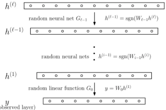
Our generative model (“ground truth”) has`hidden layers of vectors of binary variablesh(`),h(`−1), ..,h(1) (where h(`) is the top layer) and an observed layery (sometimes denoted byh(0)) at bottom (see Figure1). Each layer hasn nodes4. The weighted graph between layersiandi+ 1is
denoted byGi= (Ui, Vi, Ei, Wi). Values atUicorrespond to (h(i+1)), and those ofV
itoh(i), setEiconsists of edges between them andWi is the weighted adjacency matrix. The degree of this graph isd = nγ, and all edge weights are in[−1,1].
The samples are generated by propagating down the net-work to the observations. First sample the top layerh(`), where the set of nodes that are1is picked uniformly among all sets of sizeρ`n. We callρ`thesparsityof top level (sim-ilarlyρiwill approximately denote the sparsity of leveli). Fori=`down to2, each node in layeri−1computes a weighted sum of its neighbors in layeri, and becomes1iff that sum strictly exceeds0. We will usesgn(x)to denote
4In the full version of the paper we allow them to have differ-ent number of nodes
the threshold function that is1ifx > 0and0else. (Ap-plying sgn()to a vector involves applying it component-wise.) Thus the network computes as follows: h(i−1) = sgn(Wi−1h(i))for alli >1andy =h(0) =W0h(1)(i.e., no threshold at the observed layer).
y h(`−1)
h(1) h(`)
random neural netG`−1
random linear functionG0 y=W0h(1)
h(`−1)= sgn(W
`−1h(`))
(observed layer)
random neural nets h(i−1)= sgn(W
i−1h(i))
Figure 1.Example of a deep network
Random deep net model: We assume that in the ground truth network, the edges between layers are chosen ran-domly subject to expected degreedbeing5nγ, whereγ < 1/(`+1), and each edgee∈Eicarries a weight that is cho-sen randomly in[−1,1]. This is our modelR(`, ρ`,{Gi}). We also consider —because it leads to a simpler and more efficient learner—a model where edge weights are random in{±1} instead of [−1,1]; this is called D(`, ρ`,{Gi}). Recall thatρ` >0is such that the0/1vector input at the top layer has1’s in a random subset ofρ`nnodes.
It can be seen that since the network is random of degree d, applying aρ`n-sparse vector at the top layer is likely to produce the following density of1’s (approximately) at the successive layers: ρ`d/2, ρ`(d/2)2, etc.. We assume the density of last layerρ`d`/2`=O(1). This way the density at the last-but-one layer iso(1), and the last layer is real-valued and dense.
Now we state our main result. Note that1/ρ`is at mostn. Theorem 1 When degree d = nγ for 0 < γ
≤ 0.2, density ρ`(d/2)` = C for some large constant C6, the network model D(`, ρ`,{Gi}) can be learnt7 using O(logn/ρ2
`)samples andO(n2`)time. The network model
R(`, ρ`,{Gi})can be learnt in polynomial time and using O(n3`2logn/η2)samples8.
5
In the full version we allow degrees to be different for differ-ent layers.
6Notice that this number is roughly the expected number of features that are on and influence a particular observed variable. WhenCis a large constant the output has sparsity close to 1.
7The algorithm outputs a network that is equivalent to the ground truth up to permutation of hidden variables
8
Here the learning algorithm outputs a network; the distribu-tion generated by this output for all but the last layer is within total variation distanceηto the true distribution.
Algorithmic ideas. We are unable to analyse existing al-gorithms. Instead, we give new learning algorithms that exploit the very same structure that makes these random networks interesting in the first place i.e., each layer is a denoising autoencoder. The crux of the algorithm is a new twist on the old Hebbian rule (Hebb,1949) that “Things that fire together wire together.” In the setting of layerwise learning, this is adapted as follows: “Nodes in the same layer that fire together a lot are likely to be connected (with positive weight) to the same node at the higher layer.” The algorithm consists of looking for such pairwise (or3-wise) correlations and putting together this information globally. The global procedure boils down to the graph-theoretic problem of reconstructing a bipartite graph given pairs of nodes that share a common neighbor (see Section6). This is a variant of the GRAPH SQUARE ROOT problem which is NP-complete on worst-case instances but solvable for sparse random (or random-like) graphs.
Note that existing neural net algorithms (to the extent that they are Hebbian) can also be seen as leveraging corre-lations. But putting together this information is done via the language of nonconvex optimization (i.e., an objective function with suitable penalty terms). Our ground truth network is indeed a particular local optimum in any rea-sonable formulation. It would be interesting to show that existing algorithms provably find the ground truth in poly-nomial time but currently this seems difficult.
Can our new ideas be useful in practice? We think that using a global reconstruction procedure that leverages lo-cal correlations seems promising, especially if it avoids nonconvex optimization. Our proof currently needs that the hidden layers are sparse, and the edge structure of the ground truth network is “random like” (in the sense that two distinct features at a level tend to affectfairlydisjoint sets of features at the next level). We need this assumption both for inferring correlations and the reconstruction step. Finally, note that random neural nets do seem useful in so-called reservoir computing, and more structured neu-ral nets with random edge weights are also interesting in feature learning (Saxe et al.,2011). So perhaps they do provide useful representational power on real data. Such empirical study is left for future work.
Throughout, we need well-known properties of random graphs with expected degree d, such as the fact that they are expanders (Hoory et al.,2006); these properties appear in the supplementary material. The most important one, unique neighbors property, appears in the next Section.
3. Each layer is a Denoising Auto-encoder
As mentioned earlier, modern deep nets research often as-sumes that the net (or at least some layers in it) shouldapproximately preserve information, and even allows easy going back/forth between representations in two adjacent layers (what we earlier called “reversibility”). Below,y de-notes the lower layer andhthe higher (hidden) layer. Pop-ular choices ofsinclude logistic function, soft max, etc.; we use a simple threshold function in our model.
Definition 1 (DENOISING AUTOENCODER) An autoen-coderconsists of adecoding functionD(h) =s(W h+b) and an encoding function E(y) = s(W0y +b0) where W, W0 are linear transformations, b, b0 are fixed vectors
andsis a nonlinear function that acts identically on each coordinate. The autoencoder isdenoisingifE(D(h)+ξ) = hwith high probability wherehis drawn from the distribu-tion of the hidden layer, ξ is a noise vector drawn from the noise distribution, and D(h) + ξ is a shorthand for “D(h)corrupted with noiseξ.” The autoencoder is said to useweight tyingifW0=WT.
In empirical work the denoising autoencoder property is only implicitly imposed on the deep net by minimizing the reconstruction error||y−D(E(y +ξ))||, whereξ is the noise vector. Our definition is slightly different but is ac-tually stronger since y is exactly D(h) according to the generative model. Our definition implies the existence of an encoder E that makes the penalty term exactly zero. We show that in our ground truth net (whether from model
D(`, ρ`,{Gi})orR(`, ρ`,{Gi})) every graphGiwhp sat-isfies this definition, and with weight-tying.
We show a single-layer random network is a denoising au-toencoder if the input layer is a randomρnsparse vector, and the output layer has densityρd/2<1/20.
Lemma 2 Ifρd <0.1(i.e., the bottom layer is also fairly sparse) then the single-layer network G(U, V, E, W) in
D(`, ρ`,{Gi}) or R(`, ρ`,{Gi}) is a denoising autoen-coder with high probability (over the choice of the random graph and weights), where the noise flips every output bit independently with probability0.1. It uses weight tying. The proof of this lemma highly relies on a property of ran-dom graph, called thestrong unique-neighbor property. For any nodeu∈U, letF(u)be its neighbors inV; for any subsetS⊂U, letUF(u, S)be the set ofuniqueneighbors ofuwith respect toS, i.e.,
UF(u, S),{v∈V :v∈F(u), v6∈F(S\ {u})}
Property 1 In a bipartite graph G(U, V, E, W), a node u∈ U has(1−)-unique neighbor property (UNP) with respect toSif
X
v∈UF(u,S)
|W(u, v)| ≥(1−) X v∈F(u)
|W(u, v)| (1)
The setS has(1−)-strong UNP if every node inU has (1−)-UNP with respect toS.
Note that we don’t need this property to hold for all sets of sizeρn(which is possible ifρdis much smaller). However, for any fixed setSof sizeρn, this property holds with high probability over the randomness of the graph.
Now we sketch the proof for Lemma2 (details are in full version) when the edge weights are in{−1,1}.
First, the decoder definition is implicit in our generative model:y = sgn(W h). (That is,b=~0in the autoencoder definition.) Let the encoder beE(y) = sgn(WTy +b0)
forb0 = 0.2d
×~1.In other words, the same bipartite graph and different thresholds can transform an assignment on the lower level to the one at the higher level.
To prove this consider the strong unique-neighbor property of the network. For the set of nodes that are1at the higher level, a majority of their neighbors at the lower level are unique neighbors.The unique neighbors with positive edges will always be 1 because there are no−1edges that can cancel the +1edge (similarly the unique neighbors with negative edges will always be 0). Thus by looking at the set of nodes that are1at the lower level, one can infer the correct0/1assignment to the higher level by doing a sim-ple threshold of say0.2dat each node in the higher layer.
4. Learning a single layer network
Our algorithm, outlined below (Algorithm 1), learns the network layer by layer starting from the bottom. We now focus on learning a single-layer network, which as we noted amounts to learningnonlineardictionaries with ran-dom dictionary elements. The algorithm illustrates how we leverage the sparsity and the randomness of the edges, and use pairwise or 3-wise correlations combined with Recov-erGraph procedure of Section6.
Algorithm 1High Level Algorithm
Input: samples y’s generated by a deep network de-scribed in Section2
Output: the network/encoder and decoder functions
1: fori= 1TOldo
2: Constructcorrelation graphusing samples ofh(i−1)
3: Call RecoverGraph to learn the positive edgesE+ i
4: Use PartialEncoder to encode allh(i−1)toh(i)
5: Use LearnGraph/LearnDecoder to learn the graph/decoder between layeriandi−1.
6: end for
For simplicity we describe the algorithm when edge weights are {−1,1}, and sketch the differences for real-valued weights at the end of this section.
As before we use ρ to denote the sparsity of the hidden layer. Say two nodes in the observed layer arerelatedif they have a common neighbor in the hidden layer to which they are attached via a+1edge. The algorithm first tries to identify all related nodes, then use this information to learn all the positive edges. With positive edges we show it is already possible to recover the hidden variables. Fi-nally given both hidden variables and observed variables the algorithm finds all negative edges.
STEP1:Construct correlation graph:This step uses a new twist on the Hebbian rule to identify correlated nodes.9 Algorithm 2PairwiseGraph
Input: N =O(logn/ρ)samples ofy= sgn(W h), Output: Gˆon verticesV,u, vconnected if related
foreachu, vin the output layerdo
if≥ρN/3samples haveyu=yv= 1then connectuandvinGˆ
end if end for
ClaimIn a random sample of the output layer, related pairs u, v are both1with probability at least0.9ρ, while unre-lated pairs are both1with probability at most(ρd)2. (Proof Sketch): First consider a related pair u, v, and let z be a vertex with+1edges tou,v. Let S be the set of neighbors of u, v excluding z. The size of S cannot be much larger than2d. Under the choice of parameters, we knowρd1, so the eventhS =~0conditioned onhz = 1 has probability at least 0.9. Hence the probability ofu andvbeing both1is at least0.9ρ. Conversely, ifu, vare unrelated then for bothu, v to be1there must be nodesy andzsuch thathy =hz= 1, and are connected touandv respectively via+1edges. The probability of this event is at most(ρd)2by union bound.
Thus, if(ρd)2<0.1ρ, usingO(logn/ρ2)samples we can estimate the correlation of all pairs accurately enough, and hence recover all related pairs whp.
STEP2:Use RecoverGraph procedure to find all edges that have weight+1.(See Section6for details.)
STEP3:Using the+1edges to encode all the samplesy. Algorithm 3PartialEncoder
Input: positive edgesE+,y= sgn(W h), thresholdθ Output: the hidden variableh
Let M be the indicator matrix of E+ (M
i,j = 1 iff (i, j)∈E+)
returnh= sgn(MTy
−θ~1)
9The lowermost (real valued) layer is treated slightly differ-ently – see Section7.
Although we have only recovered the positive edges, we can use PARTIALENCODERalgorithm to gethgiveny! Lemma 3 If support of h satisfies 11/12-strong unique neighbor property, andy = sgn(W h), then Algorithm3
outputshwithθ= 0.3d.
This uses the unique neighbor property: for everyz with hz = 1, it has at least0.4dunique neighbors that are con-nected with+1edges. All these neighbors must be1 so [(E+)Ty]
z ≥ 0.4d. On the other hand, for any z with hz = 0, the unique neighbor property implies that zcan have at most0.2dpositive edges to the+1’s inh. Hence h= sgn((E+)Ty
−0.3d~1).
STEP4:Recover all weight−1edges. Algorithm 4Learning Graph
Input: positive edgesE+, samples of(h, y) Output: E−
1: R←(U×V)\E+.
2: foreach of the samples(h, y), and eachvdo
3: LetSbe the support ofh
4: ifyv= 1andS∩B+(v) ={u}for someuthen
5: For alls∈Sremove(s, v)fromR
6: end if
7: end for
8: returnR
Now consider many pairs of(h, y), wherehis found using Step 3. Suppose in some sample,yu = 1for someu, and exactly one neighbor ofuin the+1edge graph (which we know entirely) is in supp(h). Then we can conclude that for anyzwithhz= 1, there cannot be a−1edge(z, u), as this would cancel out the unique+1contribution.
Lemma 4 GivenO(logn/(ρ2d))samples of pairs(h, y), with high probability (over the random graph and the sam-ples) Algorithm4outputs the correct setE−.
To prove this lemma, we just need to bound the probability of the following events for any non-edge(x, u): hx = 1,
|supp(h)∩B+(u)
|= 1,supp(h)∩B−(u) =
∅(B+, B−
are positive and negative parents). These three events are almost independent, the first has probabilityρ, second has probability≈ρdand the third has probability almost 1. Leveraging3-wise correlation: The above sketch used pairwise correlations to recover the+1weights whenρ
1/d2. It turns out that using3-wise correlations allow us to find correlations under a weaker requirementρ <1/d3/2. Now call three observed nodes u, v, srelated if they are connected to a common node at the hidden layer via+1 edges. Then we can prove a claim analogous to the one above, which says that for a related triple, the probability
thatu, v, sare all1is at least0.9ρ, while the probability for unrelated triples is roughly at most(ρd)3. Thus as long as ρ <0.1/d3/2, it is possible to find related triples correctly. The RecoverGraph algorithm can be modified to run on 3-uniform hypergraph consisting of these related triples to recover the+1edges.
The end result is the following theorem. This is the algo-rithm used to get the bounds stated in our main theorem.
Theorem 5 Suppose our generative neural net model with weights {−1,1} has a single layer and the assignment of the hidden layer is a random ρn-sparse vector, with ρ 1/d3/2. Then there is an algorithm that runs in O(n(d3+n))time and uses O(logn/ρ2)samples to re-cover the ground truth with high probability over the ran-domness of the graph and the samples.
When weights are real numbers. We only sketch this and leave the details to the full version. Surprisingly, steps 1, 2 and 3 still work. In the proofs, we have only used the sign of the edge weights – the magnitude of the edge weights can be arbitrary. This is because the proofs in these steps relies on the unique neighbor property. If some node is on (has value 1), then its unique positive neighbors at the next level will always be on, no matter how small the positive weights might be. Also notice in PartialEncoder we are only using the support ofE+, but not the weights. After Step 3 we have turned the problem of unsupervised learning to a supervised one in which the outputs are just linear classifiers over the inputs! Thus the weights on the edges can be learnt to any desired accuracy.
5. Correlations in a Multilayer Network
We now consider multi-layer networks, and show how they can be learnt layerwise using a slight modification of our one-layer algorithm at each layer. At a technical level, the difficulty in the analysis is the following: in single-layer learning, we assumed that the higher layer’s assignment is a randomρn-sparse binary vector, however in the multilayer network, the assignments in intermediate layers do not sat-isfy this. We will show nonetheless that the the correlations at intermediate layers are low enough, so our algorithm can still work. Again for simplicity we describe the algorithm for the model D(`, ρ`,{Gi}), in which the edge weights are±1. Recall thatρi’s are the “expected” number of1s in the layerh(i). Because of the unique neighbor property, we expect roughlyρ`(d/2)fraction ofh(`−1)to be1. Hence ρi=ρ`·(d/2)`−i.Lemma 6 Consider a network fromD(`, ρ`,{Gi}). With high probability (over the random graphs between layers)
for any two nodesu, vin layerh(1), Pr[h(1)
u =h (1) v = 1]
≥ρ2/2 ifu, vrelated
≤ρ2/4 otherwise
(Proof Sketch): Call a nodesat the topmost layer an an-cestor ofuif there is a path of length`−1fromstou. The number of ancestors of a nodeuis roughly2`−1ρ
1/ρ`. With good probability there is at most one ancestor ofuthat has value 1.Callsa positive ancestor ofu, if when onlys is 1 at the topmost layer, the nodeuis 1. The number of positive ancestors ofuis roughlyρ1/ρ`.
The probability that a nodeuis on is roughly proportional to the number of positive ancestors. For a pair of nodes, if they are both 1, either one of their common positive ances-tor is 1, or both of them have a positive ancesances-tor that is 1. The probability of the latter isO(ρ2
1)which by assumption is much smaller thanρ2.
Whenu, v share a common positive parentz, the positive ancestors ofz are all common positive ancestors ofu,v (so there are at leastρ2/ρ`). The probability that one of positive common ancestor is on and no other ancestors are on is at leastρ2/2.
If u, v do not share a common parent, then the number of their common positive ancestors depends on how many “common grandparents” (common neighbors in layer 3) they have. We show with high probability (over the graph structure) the number of common positive ancestors is small. Therefore the probability that bothu,vare 1 is small.
Once we can identify related pairs by Lemma6, the Steps 2,3,4 in the single layer algorithm still work. We can learn the bottom layer graph and geth(2). This argument can be repeated after ‘peeling off’ the bottom layer, thus allowing us to learn layer by layer.
6. Graph Recovery
Graph reconstruction consists of recovering a graph given information about its subgraphs (Bondy & Hemminger, 1977). A prototypical problem is theGraph Square Root problem, which calls for recovering a graph given all pairs of nodes whose distance is at most2. This is NP-hard. Definition 2 (Graph Recovery) Let G1(U, V, E1) be an unknown random bipartite graph between |U| = n and
|V|=nnodes where each edge is picked with probability d/nindependently.
Given: GraphG(V, E)where(v1, v2) ∈ E iffv1 andv2 share a common parent inG1(i.e.∃u∈Uwhere(u, v1)∈ E1and(u, v2)∈E1).
Some of our algorithms (using 3-wise correlations) need to solve analogous problem where we are given triples of nodes which are mutually at distance 2 from each other, which we will not detail for lack of space.
We letF(S)(resp. B(S)) denote the set of neighbors of S⊆U(resp.⊆V) inG1. AlsoΓ(·)gives the set of neigh-bors in G. Now for the recovery algorithm to work, we need the following properties (all satisfied whp by random graph whend3/n
1): 1. For anyv1, v2∈V,
|(Γ(v1)∩Γ(v2))\(F(B(v1)∩B(v2)))|< d/20. 2. For anyu1, u2∈U,|F(u1)∪F(u2)|>1.5d. 3. For any u ∈ U, v ∈ V and v 6∈ F(u),
|Γ(v)∩F(u)|< d/20.
4. For anyu∈U, at least0.1fraction of pairsv1, v2 ∈ F(u)does not have a common neighbor other thanu.
The first property says “most correlations are generated by common cause”: all but possiblyd/20of the common neighbors ofv1andv2inG, are in fact neighbors of a com-mon neighbor ofv1andv2inG1.
The second property says the setsF(u)should not overlap much. This is clear because the sets are random.
The third property says if a node v is not ‘caused by’u, then it is not correlated with too many neighbors ofu. The fourth property says every cause introduces a signifi-cant number of correlations that are unique to that cause. In fact, Properties 2-4 are closely related from the unique neighbor property.
Lemma 7 When graphG1satisfies Properties 1-4, Algo-rithm5 successfully recoversG1 in expected timeO(n2). (Proof Sketch): We first show that when(v1, v2)has more than one unique common cause, then the condition in the if statement must be false. This follows from Property 2. We know the set S contains F(B(v1)∩B(v2)). If
|B(v1)∩B(v2)| ≥ 2 then Property 2 says |S| ≥ 1.5d, which implies the condition in the if statement is false. Then we show if(v1, v2)has a unique common cause u, thenS0 will be equal to F(u). By Property 1, we know
S = F(u)∪T where|T| ≤ d/20. Now, every v in F(u)is connected to every other node inF(u). Therefore
|Γ(v)∩S| ≥ |Γ(v)∩F(u)| ≥0.8d−1, andv∈S0.
For any nodev0outsideF(u), by Property 3 it can only be
connected tod/20nodes inF(u). Therefore|Γ(v)∩S| ≤ |Γ(v)∩F(u)|+|T| ≤ d/10. Hencev0is not inS0. Fol-lowing these arguments,S0must be equal toF(u), and the
algorithm successfully learns the edges related tou.
The algorithm will successfully find all nodesu∈ U be-cause of Property 4: for everyuthere are enough number of edges inGthat is only caused byu. When one of them is sampled, the algorithm successfully learns the nodeu. Finally we bound the running time. By Property 4 we know that the algorithm identifies a new nodeu∈ U in at most 10iterations in expectation. Each iteration takes at most O(n)time. Therefore the algorithm takes at mostO(n2) time in expectation.
Algorithm 5RecoverGraph Input: Ggiven as in Definition2
Output: Find the graphG1as in Definition2. repeat
Pick a random edge(v1, v2)∈E. LetS={v: (v, v1),(v, v2)∈E}. if|S|<1.3dthen
S0 =
{v ∈S :|Γ(v)∩S| ≥0.8d−1} {S0should
be a clique inG}
InG1, create nodeu, connectuto everyv∈S0. Mark all the edges(v1, v2)forv1, v2∈S0. end if
untilall edges are marked
7. Learning the lowermost (real-valued) layer
Note that in our model, the lowest (observed) layer is real-valued and does not have threshold gates. Thus our earlier learning algorithm cannot be applied as is. However, we see that the same paradigm – identifying correlations and using RecoverGraph – can be used.The first step is to show that for a random weighted graph G, the linear decoderD(h) =W hand the encoderE(y) = sgn(WTy +b) form a denoising autoencoder with real-valued outputs, as in Bengio et al. (Bengio et al.,2013). Lemma 8 IfGis a random weighted graph, the encoder E(y) = sgn(WTy
−0.4d~1)and linear decoderD(h) = W h form a denoising autoencoder, for noise vectors γ which have independent components, each having variance at mostO(d/log2n).
The next step is to show a bound on correlations as before. For simplicity we state it assuming the layerh(1)has a ran-dom0/1assignment of sparsityρ1. In the full version we consider the correlations introduced by higher layers as we did in Section5.
Theorem 9 Whenρ1d=O(1),d= Ω(log2n), with high probability over the choice of the weights and the choice of the graph, for any three nodesu, v, sthe assignmenty to the bottom layer satisfies:
1. If u, v and s have no common neighbor, then
2. If u, v and s have a unique common neighbor, then
|Eh[yuyvys]| ≥2ρ1/3
8. Two layers are more expressive than one
In this section we show that a two-layer network with±1 weights is more expressive than one layer network with ar-bitrary weights. A two-layer network(G1, G2)consists of random graphsG1andG2with random±1weights on the edges. Viewed as a generative model, its input ish(3) and the output ish(1) = sgn(W1sgn(W2h(3))). We will show that a single-layer network even with arbitrary weights and arbitrary threshold functions must generate a fairly differ-ent distribution.
Lemma 10 For almost all choices of(G1, G2), the follow-ing is true. For every one layer network with matrix A and vectorb, ifh(3) is chosen to be a randomρ
3n-sparse vector withρ3d2d1 1, the probability (over the choice of h(3)) is at least Ω(ρ2
3) that sgn(W1sgn(W2h(3))) 6= sgn(Ah(3)+b).
The idea is that the cancellations possible in the two-layer network simply cannot all be accomodated in a single-layer network even using arbitrary weights. More precisely, even the bit at a single output nodevcannot be well-represented by a simple threshold function.
First, observe that the output atvis determined by values of d1d2 nodes at the top layer that are its ancestors. It is not hard to show in the one layer net(A, b), there should be no edge between v and any node uthat is not its an-cestor. Then consider structure in Figure2. Assuming all other parents of v are 0 (which happens with probability at least 0.9), and focus on the values of (u1, u2, u3, u4). When these values are(1,1,0,0)and(0,0,1,1),v is off. When these values are(1,0,0,1)and(0,1,1,0),v is on. This is impossible for a one layer network because the first two ask forP
Aui,v+2bv ≤0and the second two ask for P
Aui,v+2bv<0.
h(1)
h(2)
v
+1 -1
+1
u1 u2 u3
h(3)
+1
+1
G2
G1 s s0
u4
-1
Figure 2.Two-layer network(G1, G2)
9. Experiments
We did a basic implementation of our algorithms and ran experiments on synthetic data. The results show that our analysis has the right asymptotics, and that the constants involved are all small. As is to be expected, the most ex-pensive step is that of finding the negative edges (since the
algorithm is to ‘eliminate non-edges’). However, stopping the algorithm after a certain number of iterations gives a reasonable over-estimate for the negative edges.
The following are the details of one experiment: a network with two hidden layers and one observed layer (`= 2, both layers use thresholds) withn= 5000,d= 16andρ`n= 4; the weights are random{±1}but we made sure that each node has exactly8positive edges and8negative edges. Us-ing 500,000 samples, in less than one hour (on a single 2GHz processor) the algorithm correctly learned the first layer, and the positive edges of the second layer. Learn-ing the negative edges of second layer (as per our analysis) requires many more samples. However using5×106 sam-ples, the algorithm makes only 10 errors in learning nega-tive edges.
10. Conclusions
Many aspects of deep nets are mysterious to theory: re-versibility, why use denoising autoencoders, why this highly non-convex problem is solvable, etc. Our paper gives a first-cut explanation. Worst-case nets seem hard, and rigorous analysis of interesting subcases can stimu-late further development: see e.g., the role played in Bayes nets by rigorous analysis of message-passing on trees and graphs of low tree-width. We chose to study randomly erated nets, which makes scientific sense (nonlinear gen-eralization of random error correcting codes, compressed sensing etc.), and also has some empirical support, e.g. in reservoir computing.
The very concept of a denoising autoencoder (with weight tying) suggests to us a graph with random-like properties. We would be very interested in an empirical study of the randomness properties of actual deep nets learnt via super-vised backprop. (For example, in (Krizhevsky et al.,2012) the lower layers use convolution, which is decidedly non-random. But higher layers are learnt by backpropagation initialized with a complete graph and may end up more random-like.)
Network randomness is not so crucial in our analysis of learning a single layer, but crucial for layerwise learning: the randomness of the graph structure is crucial for con-trolling (i.e., upper bounding) correlations among features appearing in the same hidden layer (see Lemma6). Prov-able layerwise learning under weaker assumptions would be very interesting.
Acknowledgements
We would like to thank Yann LeCun, Ankur Moitra, Sushant Sachdeva, Linpeng Tang for numerous helpful dis-cussions throughout various stages of this work and anony-mous reviewers for their helpful feedback and comments.
References
Anandkumar, Anima, Foster, Dean P., Hsu, Daniel, Kakade, Sham M., and Liu, Yi-Kai. A spectral algorithm for latent Dirichlet allocation. InAdvances in Neural In-formation Processing Systems 25, 2012.
Arora, Sanjeev., Ge, Rong., and Moitra, Ankur. Learning topic models – going beyond svd. InIEEE 53rd Annual Symposium on Foundations of Computer Science, FOCS 2012, New Brunswick NJ, USA, October 20-23, pp. 1– 10, 2012.
Arora, Sanjeev, Ge, Rong, and Moitra, Ankur. New algo-rithms for learning incoherent and overcomplete dictio-naries. ArXiv, 1308.6273, 2013.
Bengio, Yoshua. Learning deep architectures for AI. Foun-dations and Trends in Machine Learning, 2(1):1–127, 2009. Also published as a book. Now Publishers, 2009. Bengio, Yoshua, Courville, Aaron C., and Vincent,
Pas-cal. Representation learning: A review and new per-spectives. IEEE Trans. Pattern Anal. Mach. Intell., 35 (8):1798–1828, 2013.
Berinde, R., Gilbert, A.C., Indyk, P., Karloff, H., and Strauss, M.J. Combining geometry and combinatorics: a unified approach to sparse signal recovery. In46th An-nual Allerton Conference on Communication, Control, and Computing, pp. 798–805, 2008.
Bondy, J Adrian and Hemminger, Robert L. Graph recon-structiona survey. Journal of Graph Theory, 1(3):227– 268, 1977.
Cho, Youngmin and Saul, Lawrence. Kernel methods for deep learning. InAdvances in Neural Information Pro-cessing Systems 22, pp. 342–350. 2009.
Donoho, David L. Compressed sensing. Information The-ory, IEEE Transactions on, 52(4):1289–1306, 2006. Hebb, Donald O. The Organization of Behavior: A
Neu-ropsychological Theory. Wiley, new edition edition, June 1949.
Hoory, Shlomo, Linial, Nathan, and Wigderson, Avi. Ex-pander graphs and their applications. Bulletin of the American Mathematical Society, 43(4):439–561, 2006. Hsu, Daniel and Kakade, Sham M. Learning mixtures of
spherical gaussians: moment methods and spectral de-compositions. InProceedings of the 4th conference on Innovations in Theoretical Computer Science, pp. 11– 20, 2013.
Hsu, Daniel, Kakade, Sham M., and Zhang, Tong. A spec-tral algorithm for learning hidden Markov models. Jour-nal of Computer and System Sciences, 78(5):1460–1480, 2012.
Jackson, Jeffrey C, Klivans, Adam R, and Servedio, Rocco A. Learnability beyondac0. InProceedings of the thiry-fourth annual ACM symposium on Theory of computing, pp. 776–784. ACM, 2002.
Klivans, Adam R and Sherstov, Alexander A. Crypto-graphic hardness for learning intersections of halfspaces. Journal of Computer and System Sciences, 75(1):2–12, 2009.
Krizhevsky, Alex, Sutskever, Ilya, and Hinton, Geoff. Im-agenet classification with deep convolutional neural net-works. InAdvances in Neural Information Processing Systems 25, pp. 1106–1114. 2012.
Livni, Roi, Shalev-Shwartz, Shai, and Shamir, Ohad. A provably efficient algorithm for training deep networks. ArXiv, 1304.7045, 2013.
Moitra, Ankur and Valiant, Gregory. Settling the polyno-mial learnability of mixtures of gaussians. In the 51st Annual Symposium on the Foundations of Computer Sci-ence (FOCS), 2010.
Saxe, Andrew, Koh, Pang W, Chen, Zhenghao, Bhand, Maneesh, Suresh, Bipin, and Ng, Andrew. On random weights and unsupervised feature learning. In Proceed-ings of the 28th International Conference on Machine Learning (ICML-11), pp. 1089–1096, 2011.
Vincent, Pascal, Larochelle, Hugo, Bengio, Yoshua, and Manzagol, Pierre-Antoine. Extracting and composing robust features with denoising autoencoders. InICML, pp. 1096–1103, 2008.