978-1-5386-5457-6/18/$31.00 ©2018 IEEE
Sonar-based SLAM Using Occupancy Grid Mapping
and Dead Reckoning
Muhammad S. A. Khan Department of Electrical and Electronic
Engineering BRAC University Dhaka, Bangladesh
Shoumik S. Chowdhury Department of Computer Science and
Engineering BRAC University Dhaka, Bangladesh [email protected] acu.ac.bd Nafis Niloy
Department of Mathematics and Natural Science
BRAC University Dhaka, Bangladesh [email protected] Fatema Tuz Zohra Aurin
Department of Computer Science and Engineering BRAC University
Dhaka, Bangladesh [email protected]
Tarem Ahmed
Department of Computer Science and Engineering Independent University, Bangladesh (IUB)
Dhaka, Bangladesh [email protected] Abstract— This paper presents a solution for Simultaneous
localization and mapping (SLAM) with an autonomous differential drive robot in an indoor environment. We extract data from sonars and analyze it to construct a map of the explored area using occupancy grid mapping. In addition, relative positioning approaches provide location using an inertial measurement unit (IMU) and wheel encoders. Localization and mapping are essential tasks for an autonomous robot's navigation or exploration without a prior map and the system is based on discrete step-wise or event modeling which guides its navigation. The system’s result is compared for accuracy against an actual map. The results show that the approach is largely accurate although the resolution of the map produced could be improved.
Keywords— occupancy grid map, dead reckoning, Simultaneous localization and mapping
I. INTRODUCTION
Simultaneous localization and mapping or SLAM is a key problem within mobile robotics as it can provide a way towards truly autonomous robots or vehicles [1][2]. SLAM is the problem in which a mobile robot when placed in an unknown environment must find a way to explore and navigate around the environment to produce a map of the environment and at the same time to estimate its position by only using onboard sensors [3]. A robot given a prior map would not have too much of a problem figuring out its location within the environment by recognizing specific features. Similarly, a robot which is given accurate position data would be able to produce a map of the environment. The main difficulty in SLAM lies in the absence of both accurate data on the map of its environment or position within it.
The Kalman Filter is frequently used in probabilistic robotics and has been modified for non-linear systems to the Extended Kalman Filter (EKF), which expanded filtering approaches since its introduction in [4] as a method to incrementally estimate the posterior distribution over the robot pose and the
positions of landmarks. Other filters used are the Extended Information Filter [5] and the Particle filter [6].
The SLAM problem is usually solved using laser or vision based approaches applied on metric or topological maps [7][8]. Our approach, in contrast, uses sonar sensor and occupancy grid mapping to map environments. In addition, an inertial measurement unit (IMU) and wheel encoders are used for relative positioning. This allows us to formulate a navigation and exploration algorithm for traversing the environment until a complete map is made. The solution uses sonars but with an optimized trade-off between computational complexity, expensiveness, and accuracy.
This paper is organized into several sections. In section II, past research work and related papers are discussed. Section III explains the core algorithm at work: the approaches taken for localization and mapping are discussed separately, exploration strategy to traverse the environment is outlined and the method for graphical representation of the complete map is illustrated. In section IV, the results of the experiment of the implementation are compared with a known map and finally, section V summarizes the thesis and discusses the future applications and work along with limitations in our experiment.
II. PRIOR WORK
A lot of the work done on SLAM is done with laser scanners or lidars such as in the case of [9], [10], and [11]. Apart from the use of lidars, a web camera is used in [12] to extract Scale Invariant Features Transform (SIFT) to help with indoor navigation help for blind people. Cameras are also used in [13] and [14]. In [13] a single camera is used to produce a map and do localization, and in [14] a kinect depth camera is used in conjunction with WiFi localization. In contrast, in [15] a 3D map from lidar data is used but localization is done using a monocular camera. However, in this section and throughout the rest of this paper, we focus on approaches to the problem that could employ sonar or ultrasonic sensors instead.
In one such case, like in [16], an onboard Arduino controls a rover while it is sent control commands by a Raspberry Pi which carries out a SLAM algorithm based on the EKF and Random Sampling Consensus (RANSAC) techniques. It was designed to extract two types of landmarks (straight lines and spikes). A Laptop, in turn, communicates with the Raspberry Pi through wireless communication. The rover reports two different types of events; its change in odometry and the results of a scan during which the rover collects 180-degree readings from its servo mounted sonar.
Another implementation where sonar sensors are used is in [17] where an Arduino is responsible for collecting sensor data and sending it to a computer. The Arduino receives control commands from the computer and works as the onboard controller for the rover. The rover includes four motors and encoders, an Arduino Mega, three sonar sensors and an IMU. A probabilistic occupancy grid mapping and a simple edge following map making strategy are employed where the robot tries to drive past obstacles at a short distance until all obstacles have been visited.
Occupancy grid mapping is used in [18] where low-cost robots using infrared proximity sensors for obstacle detection and an ultrasonic beacon system in addition to wheel encoders is used for localization. Due to restrictions in computing power, an optimized Backtracking Occupancy Grid-Based Mapping or BOBMapping algorithm is used on a field programmable gate array or FPGA robot. The algorithm also optimizes exploration of the surrounding. The robot divides the area to be mapped into grids and explores based on the information available about the grids, such as whether they are occupied or unoccupied and whether they are charted or uncharted. The
algorithm is shown in action in Figure 1. This along with backtracking allows the robot to fully explore its environment and produce an occupancy grid map as a result.
Dead reckoning, as used for localization in [19], takes the initial position and the initial orientation and computes a relative position from them incrementally over time. Here, odometry and Inertial navigation systems (INS) are combined for relative positioning of a mobile robot. Wheel encoders are used for odometry in which the data on the rate of wheel revolutions for each of the two wheels on a differential drive robot provides the position of the robot. Encoder information as used in the odometry calculations leads to systematic and non-systematic errors. INS use an IMU to continuously update both orientation and position information; it is stable over the short term but becomes unstable over time with the accumulation of errors through the integration of outputs. To compensate for the errors in the two methods, a linear Kalman filter is designed as shown in Figure 2. No absolute positioning system is used in conjunction and the system is shown to be reliable in its localization estimations, although it has a large variance.
III. SLAM
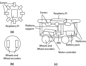
The hardware implementation as shown in Figure 3 utilizes a Raspberry Pi for main controller. There are eight sonars divided between 360 degrees for a complete view of the nearby environment. Instead of a sonar on a rotating actuator, since actuator error is to be accounted, this approach provides less uncertainty in readings. There are also wheel encoders placed within the wheels as well as an IMU at the center of the robot. The wheels would be controlled using a motor controller.
The SLAM approach is divided into three parts: Relative positioning with Kalman filter (using IMU and wheel encoder odometry data), Occupancy grid mapping using sonars and Navigation and Exploration based on stepwise update of path.
The process works in incremental steps in which the robot reads its localization sensors (IMU, wheel encoder) and updates its position in each measurement. The sonars measurements are Figure 2: Design of a linear Kalman Filter used for dead reckoning [19]
Figure 1: BOBMapping algorithm at work with robot choosing its next movement for three scenarios [18]
Figure 3: Robot diagram with (a) top view showing eight sonars spread over 360 degrees and Raspberry Pi, (b) bottom view of wheels and wheel encoders, and (c) all the components and their placement within the two platforms of the robot
done at the same time for a complete sweep of the sensors. This information is handled by the Occupancy grid map and Relative positioning algorithms. This completes a step for the robot after it reaches its trajected position within the map. Then the navigation algorithm decides the next trajected step. The system continues in this way until termination conditions are fulfilled.
The overall implementation is shown in Algorithm 1 and 2. Algorithm 1 initiates all its variables and calls Algorithm 2. Algorithm 2 continuously updates sensor data as well as pose and occupancy data. Algorithm 1 uses data from Algorithm 2 for navigation and exploration until it terminates operation. The algorithm will only terminate if all the grey cells are bounded by black cells, or if the last update in occupancy grid happened before a specified time limit.
A. Relative positioning
The IMU readings are used to derive velocity, position, and orientation of the robot. The wheel encoder is the system that converts the angular rate of the rotor into a digital signal. The encoders are attached to the wheels of the mobile robot; the wheel’s rotary angle is measured by the encoder. The rotor
encoder generates forty-eight counts while the wheel rotates 360 degrees. This information on the acceleration of the robots’ wheels along with the wheel radius and inter-wheel distance are used to calculate the mobile robots’ yaw angle rate.
The algorithm is based on the same approach as shown in [19] with some changes for the differences in hardware and function. The inputs from INS and odometry are made in the same manner as in Figure 2 to derive the outputs of the Kalman filter. The position of the robot is updated continuously through relative positioning as the robot moves from initial position to subsequent positions.
B. Occupancy Grid Mapping
Given the robot location and pose, the robot having a sense of its body dimensions provides its measurements from its eight sonars. These measurements update the occupancy grid map through a transform applied to the robot’s location and the location of the occupied cell. The right and left exit degrees are known to us and the arc that falls within the occupancy grid as considered occupied. The arc is simplified as the normal of the reading taken over the viewing angle of the sonar.
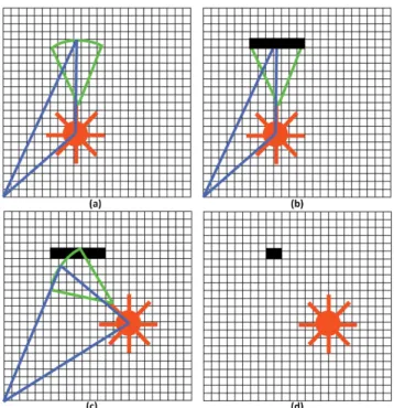
Figure 4 shows the occupancy grid map procedure. It shows the robot updating the grid once it has the view from another vantage point keeping only the union of the two observances as occupied. The sonar has a viewing angle, hence any object within that angle could be the cause of the reading. It is quite possible for some of these now occupied cells to be vacant. This is verified by using another reading if the robot is in another vantage point in its subsequent motion. It now takes another reading and the union of the two cells is taken to be the updated occupied cells, with the rest being shown as vacant.
Algorithm 1: SLAM algorithm using Occupancy Grid Mapping and Dead Reckoning
1. Initialize Sensors, State and Map update algorithm 2. Initialize Navigation thread for backtracking 3. Loop (until all grey cells are bounded by black cells
or time elapsed since last Occupancy grid update is greater than Time limit):
4. Read pose and Occupancy grid map from file 5. Check neighboring cells and Backtracking thread 6. Update motion vector and Backtracking thread 7. Set wheel control to motion vector
8. Stop wheels when it moves onto next cell 9. End Loop
Algorithm 2: Sensors, State and Map update algorithm 1. Initialize Sensors, Occupancy grid map with
resolution and map dimension data
2. Loop (until all grey cells are bounded by black cells
or time elapsed since last Occupancy grip update is greater than Time limit):
3. Update sensor data file
4. Get pose data from IMU and Wheel encoder using Kalman Filter
5. Transform relative pose into global coordinates 6. Get occupancy grid data using sonar data and
relative position
7. If grids overlap with previous grids 8. Find union of grids
9. Update Occupancy grid map 10. Else
11. Update Occupancy grip map 12. End Loop
Figure 4: Robot (magnified for easier viewing) performing (a) initial measurement, (b) selection of occupied grids, (c) moving onto another vantage point to observe a different set of occupied grids, and (d) finding overlap of grids for more accurate occupancy reading
The robot would not, however, update a cell that it has found to be empty before but is occupied now. This is because the robot is trying to determine which cells are really occupied due to the viewing angle being so large. The occupancy grid is represented using a two-dimensional array. This array is initialized with null values. Occupied cells are assigned the value 1, and unoccupied the value 0 as array is updated.
C. Navigationg and Exploration
The robot can be turned right by turning the right wheel forward and left wheel backward and vice versa using high or low values for the motor controller using its connected GPIO pin. The movement of the robot is 45 degree turns and linear movements equal to the resolution. An important aspect of Occupancy Grid Mapping is defining the resolution or minimum size of each cell. The smaller the size of the cell, the better is the mapping. However, defining a very small resolution would require a lot of memory space and would be
more complex. Therefore, the resolution is determined to be greater than the diameter of the robot in addition to the turning radius of the robot. Our resolution is 20cm where the robot diameter is 12.75cm and turning radius is 7cm.
The BOBMapping approach in [18] inspired our implementation of the navigation and exploration algorithm. The exploration would have to ensure that all accessible cells are either visited or sensed to be inaccessible. In the grid, a neighbor is said to be a cell that is immediately adjacent to each other. In the event of two or possible neighbors that the robot can visit, clockwise priority is maintained. Backtracking ensures the other possibilities are visited later.
D. Graphical representation of map
The occupancy grid map array produced once the mapping is complete is used to plot the graphical map. The map is plotted using different colored cells depending on values of the Figure 5: The surveyed map of the actual environment and the dimensions and placement of the objects in (a) Room 1, (b) Room 2, (c) Room 3, and (d) Room 4
Figure 6: The expected occupancy grid map produced from the survey for (a) Room 1, (b) Room 2, (c) Room 3, and (d) Room 4
Figure 7: The actual resulting occupancy grid map after running the SLAM algorithm and letting the mobile robot to complete its exploration of the environment for (a) Room 1, (b) Room 2, (c) Room 3, and (d) Room 4
cells. We are plotting the occupied cells as black (1 valued cells), the unexplored as gray (null valued cells), and the unoccupied as white (0 valued cells).
IV. EXPERIMENT AND RESULTS A. Experimental Set-up
The experiment was carried out in four rooms with Room 1 of size 329 by 460cm, Room 2 of size 305 by 315cm, Room 3 of size 326 by 432cm, and Room 4 of size 305 by 459cm. The rooms were surveyed to make and the actual map of the environment that the robot would carry out the SLAM algorithm in.
Room 1 is an empty room to test for conditions where the environment is without obstacles. Room 2 contains elliptical objects and rotated rectangular objects as well. In contrast, Room 4 and 3 is straight forward as a map and contains rectangular object placed closer to the walls.
Although the main SLAM algorithm runs and terminates to produce the resulting map of the environment. The N × M matrix (Room 1: 17 × 23, Room 2: 16 × 16, Room 3: 17 × 22, and Room 4: 16 × 23 matrices all of resolution 20 by 20cm) is plotted. The time limit since the last time there was an occupancy grid map update that the robot waits before terminating the algorithm is set to 20 minutes The rooms used for this experiment is shown in Figure 5 and the expected occupancy grid map in Figure 6.
B. Results and Evaluation
The results are shown in Figure 7. The map is within an acceptable range of accuracy given the resolution of the cells. However, it does have the error in occupancy showing occupied cells where it should not as in Room 1, 3 and 4 results as shown in Figure 7(a), 7(c) and 7(d) and failing to navigate a part of the environment as in Room 2 results as shown in Figure 7(b). The comparison of the results with the expected
results is shown in Table 1 and in Figure 8. The maps range in complexity and overall dimension; to compare we use a metric for error comparison. It is defined as,
Error ratioA = (EA/NA)(TA /Tavg) (1) Where Error ratio for map A is calculated with values EA
for Number of cell errors for map A, NA for total number of non-vacant cells for map A, TA for Total cells for map A, and Tavg for the average value of total cells of all the maps. Higher values indicate worse performance.
Using this value, we can make a fair comparison of all the maps since the value is normalized due to the use of Tavg and Number of cell errors is compared against total non-vacant cells. We are taking total non-vacant cells for the ratio since errors arise out of localization or sonar uncertainty and the more obstacles in the map, the higher its complexity. Essentially, we are using error ratio as a way to compare how for a normalized map our method fares against rising number of obstacles. A cell error here is taken to be any mismatch between predicted and observed map including grey cells.
However, grey cells are for the most part taken to mean inaccessible and hence essentially the same as black cells for a robot who would use our produced map to traverse the environment. Hence, we also compare Precision and F1 scores. To calculate these, we consider grey as black. Taking black and grey as being the positive condition and white as being the negative condition we are able to get our recall, precision, and F1 score.
Recall is the ratio between correct positive observations and actual number of positive observations. Our recall value for all maps is 1, meaning there are no false negatives therefore we do not produce a white cell in the place of a black or grey one. This is to our advantage since obstacle avoidance is maintained, the robot would not go to an occupied cell mistakenly thinking it is vacant.
Precision is the ratio between correct positive observations (or in our case correctly observed non-vacant cells) and total positive observations (or the sum of correctly observed non-vacant cells and incorrectly observed non-non-vacant cells). Precision unlike recall is not 1 for the maps, the errors in the maps are false positives as opposed to false negatives, that is, there are observed black cells where a white cell should be. This is most likely the outcome of accumulated error from localization or sonar error. However, the false positive errors are not significant and precision is consistent and close to 1.
TABLE I. F1SCORE,PRECISION AND ERROR RATIO FOR COMPARISON BETWEEN RESULTING MAP AND PREDICTED MAP
Map Number of cell errors Total non-vacant cells Error
ratio Precision F1 score
Room 1 1 6 0.1877 0.86 0.92
Room 2 38 106 0.2643 0.85 0.92
Room 3 7 149 0.0506 0.97 0.98
Room 4 16 242 0.0701 0.98 0.99
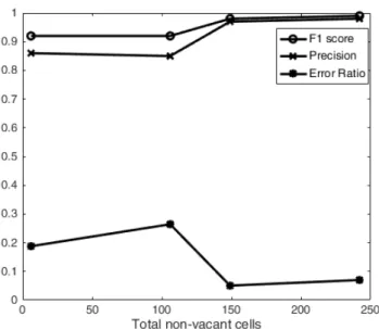
Figure 8: F1 score, Precision and Error values against Total non-vacant cells
The F1 score or the harmonic average of the precision and recall is a measure of a tests performance. Therefore, in our case F1 score evaluates how well the robot observes and determines correct values for occupancy in cells. The precision and F1 score for all maps as seen in Table 1 and Figure 8 is consistent and close to 1 throughout. Thus, our algorithm maintains high precision and performance on a consistent basis.
However, these scores do not account for overall cell errors as explained and we can look at the error ratio for a comparison for that. Room 1 was mildly accurate with 0.1877 error ratio; the performance is in line with expectations. Room 2 results show more inaccurate results (0.2643 error ratio) in terms of capturing the shapes of the objects in the environment, however, this is expected given their irregularity. Room 3 is very accurate with a 0.0506 error ratio albeit with some notable errors. While, Room 4 results are mostly accurate as well with error ratio of 0.0701. Some translation in mapping values indicating localization error is also noticed in Room 4 with some of the same error types as in Room 3. The error ratio seems to be higher for maps with irregular shapes as in Room 2. Otherwise, the results are fairly accurate.
V. CONCLUSION AND FUTURE WORK
In this paper, we have discussed and implemented the SLAM problem. The purpose of this paper was to implement SLAM in the most inexpensive way possible. The proposed method uses Kalman filter for localization and occupancy grid mapping using several ultrasonic range sensors, an IMU and wheel encoders. The entire process is carried out in discrete steps and along with occupancy grid map, makes the navigation much simpler and reduces error. The experiment shows the resulting map of the environment within an acceptable threshold of error. The resulting maps provide accurate representation of object placement within an occupancy grid. The performance is also very consistent over a number of maps albeit with difficulties in maps with complex or irregular shapes and complex placement of objects within the map. The resolution, nevertheless, could be smaller and is an area of improvement and could at the same time help with more complex maps.
Even though using ultrasonic range sensors are inexpensive compared to lidar or vision-based approaches, they inherently introduce significant noise into the environment. Another limitation is the loop closure problem, where the robot comes back to a previously-visited position but with the accumulation of errors, the robot would think it is a previously unexplored area. The robot should recognize a position it has visited before and use the new information to update the position. The other limitation is to do with a lack of any features within the map, a hybrid approach for both grid based and feature based SLAM can be implemented in the future. The approach presented in this paper requires more testing and improvement through further study to widen its application.
An interesting development in robotics is multi-robotic approaches. Decentralized approaches in general have a lot of advantages such as robustness and scalability. Future work could include a realization of SLAM using multi-robots such as in [20], and [21] for low cost robots.
REFERENCES
[1] S. Thrun, "Robotic Mapping: A Survey", Exploring Artificial Intelligence in the New Millennium, 2002.
[2] G. Dissanayake, P. Newman, S. Clark, H.F. Durrant-Whyte, and M. Csorba. A solution to the simultaneous localization and map building (SLAM) problem. IEEE Transactions of Robotics and Automation, 2001.
[3] J. Aulinas, Y. Petillot, J. Salvi, and X. Llado, "The slam problem: a survey," in Proceedings of the 2008 conference on Artificial Intelligence Research and Development, pp. 363-371, 2008.
[4] R. Cheeseman, P. Smith, "On the representation and estimation of spatial uncertainty", Int. J. Robot. Res., 1986.
[5] R. Eustice, M. Walter, J. Leonard, "Sparse extended information filters: Insights into sparsification", Proc. IEEE/RJS Int. Conf. Intell. Robots Syst., pp. 3281-3288, 2005-Aug.-2--6.
[6] M. Montemerlo, S. Thrun, D. Koller, B. Wegbreit, "FastSLAM 2.0: An improved particle filtering algorithm for simultaneous localization and mapping that provably converges", Proc. International Joint Conference on Artificial Intelligence, pp. 1151-1156, 2003.
[7] H. Durrant-Whyte, T. Bailey, "Simultaneous localization and mapping (SLAM): Part I the essential algorithms", IEEE Robot. Autom. Mag., vol. 13, no. 2, pp. 99-110, Jun. 2006.
[8] T. Bailey and H. Durrant-Whyte, "Simultaneous localisation and mapping (SLAM): Part II state of the art," Robotics & Automation Magazine, Sep 2006.
[9] A. Eliazar and R. Parr, “DP-SLAM: Fast, robust simultaneous localization and mapping without predetermined landmarks,” in Proc. 18th IJCAI’03, Aug. 2003, pp. 1135–1142.
[10] D. Hähnel, W. Burgard, D. Fox, and S. Thrun, “An efficient FastSLAM algorithm for generating maps of large-scale cyclic environments from raw laser range measurements,” in Proc. IEEE/RSJ IROS’03, Oct. 2003, pp. 206–211.
[11] W. Hess, D. Kohler, H. Rapp, D. Andor, "Real-time loop closure in 2D LIDAR SLAM", Robotics and Automation (ICRA) 2016 IEEE International Conference on, pp. 1271-1278, 2016.
[12] A. M. Ali and M. J. Nordin, “SIFT based monocular SLAM with multi-clouds features for indoor navigation,” in IEEE Region 10 Annual International Conference, Proceedings/TENCON, 2010, pp. 2326–2331. [13] I. D. Reid, A. J. Davison, O. Stasse and N. D. Molton, "MonoSLAM:
Real-Time Single Camera SLAM," in IEEE Transactions on Pattern Analysis & Machine Intelligence, vol. 29, no. 6, pp. 1052-1067, 2007. [14] P. Mirowski, R. Palaniappan, T. K. Ho, B. Labs, M. Avenue, M. Hill,
"Depth Camera SLAM on a Low-cost WiFi Mapping Robot", vol. 1, no. 908, pp. 0-5
[15] T. Caselitz, B. Steder, M. Ruhnke, W. Burgard, "Monocular camera localization in 3d lidar maps", 2016 IEEE/RSJ Int. Conf on Intelligent Robots and Systems (IROS), pp. 1926-1931, Oct 2016.
[16] P. Butterly, J. Daly and L. Morrish, "Implementing Odometry and SLAM Algorithms on a Raspberry Pi to Drive a Rover", Bachelor of Science in Computing, Institute of Technology Blanchardstown, 2014. [17] S. Theophil, "An Arduino-based mapping vehicle", GitHub, 2015.
[Online]. Available: https://github.com/stheophil/MappingRover [18] D. Gonzalez-Arjona, A. Sanchez, F. López-Colino, A. de Castro, J.
Garrido, "Simplified Occupancy Grid Indoor Mapping Optimized for Low-Cost Robots", ISPRS International Journal of Geo-Information, vol. 2, pp. 959, 2013.
[19] B.-S. Cho, W. Moon, W.-J. Seo, and K.-R. Baek, "A dead reckoning localization system for mobile robots using inertial sensors and wheel revolution encoding," J. Mech. Sci. Technol., vol. 25, no. 11, pp. 2907-2917, Nov. 2011.
[20] S. Thrun, Y. Liu, "Multirobot SLAM with sparse extended information filters" in Proc. 11th Int. Symp. Robot. Res. (ISRR'03), Italy, Sienna: Springer-Verlag, pp. 114-141.
[21] X. S. Zhou, S. I. Roumeliotis, "Multi-robot SLAM with unknown initial correspondence: The robot rendezvous case", Proc. IEEE/RSJ Int. Conf. Intell. Robots Syst., pp. 1785-1792, 2006-Oct.-915.