Enhancing eQTL analysis techniques with special attention to the transcript dependency structure

(1)

Enhancing eQTL Analysis Techniques with Special Attention

to the Transcript Dependency Structure

by

John C. Schwarz

A dissertation submitted to the faculty of the University of North Carolina at Chapel Hill in partial fulfillment of the requirements for the degree of Doctor of Philosophy in the Department of Biostatistics.

Chapel Hill 2010

Approved by:

Co-advisor: Dr. Wei Sun

Co-advisor: Dr. Fred Wright

Reader: Dr. Yun Li

Reader: Dr. Robert Millikan

(2)

c

2010

(3)

Abstract

JOHN C. SCHWARZ: Enhancing eQTL Analysis Techniques with Special Attention to the Transcript Dependency Structure.

(Under the direction of Dr. Wei Sun and Dr. Fred Wright.)

Gene expression microarray analysis and genetic marker association studies are two

com-mon experimental methods in the genetic literature. A growing number of studies have begun

combining these two experiments into a single study known as an expressed quantitative trait

loci (eQTL) study. Analysis of eQTL data has been performed on several different

organ-isms including yeast, maize, mouse, and human. We propose a set of methods to effectively

analyze eQTL data by properly transforming and adjusting analysis models. Our method

ad-dresses multiple issues often left out of eQTL analysis that include population stratification

and adjustment of racial and ethnic classifications, adjustment of multiple covariates, and

the influence of extreme outlying observations. Additionally we propose a statistic that is

able to provide significance for trans bands (i.e., genetic markers that harbor a large number

of eQTL) without the computational intensity of permutation testing. Most methods that

identify a significance threshold for trans band activity either use simple binning approaches

or have complex statistical methods that may require many assumptions and restrictions.

We use a parametric approach that uses known distributions and simple approximations to

develop a significance threshold. The advantages of our methods are that they account for

correlation structures in the gene expression data and correlation between genetic markers.

Also by using a parametric approach we do not rely on permutation testing which can be

computationally daunting for even modestly sized studies.

In the second part we will focus in on multiple testing in genetic applications. We study the

family-wise error control by quantifying the probability that our test statistic crosses a defined

threshold. The existing methods that employ this technique leave room for adjustments

(4)

of considering discoveries as clumps of genetic markers instead of individual markers. By

considering a clump as a single discovery, we can redefine the false discovery rate in terms

of clumps and not single hypotheses. Additionally we provide some modifications to better

model complex correlation structures as well as handle situations in which limited information

(5)

Acknowledgments

I would like to extend my thanks and gratitude to my advisor Dr. Fred Wright. He introduced

me to the idea of eQTL analysis and the ideas addressed in this work. I would also like to

thank Dr. Wei Sun for his involvement early in the research. He provided key insights

during numerous meetings and discussions throughout the research and written phase of this

dissertation.

I would also like to thank the other members of my committee for their guidance and

support. Their knowledge and expertise in the field of statistical genetics and genetic

epi-demiology was crucial in refining the presentation of the following work.

Finally I would like to thank my family for their support throughout my graduate work,

(6)

List of Figures

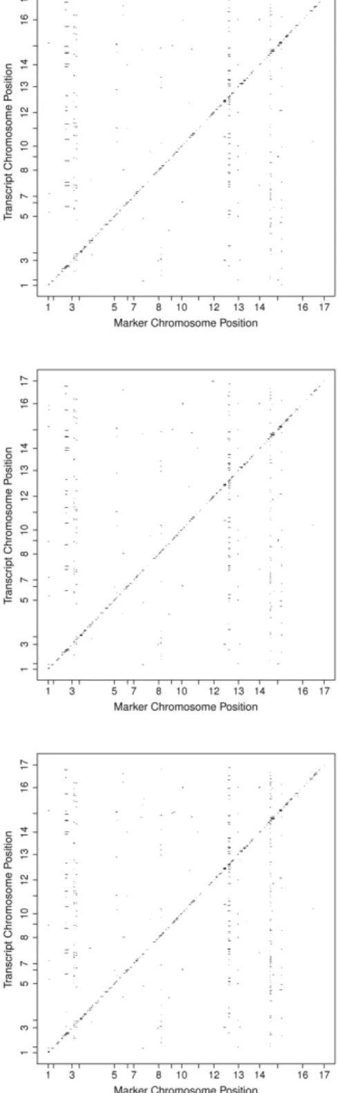
2.1 eQTL results of the Yeast from the raw data (top panel), from the transformed data (middle panel) and from the transformed and adjusted data (bottom panel) 31

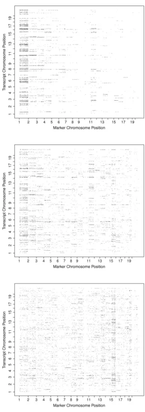
2.2 eQTL results of the Mouse from the raw data (top panel), from the transformed data (middle panel) and from the transformed and adjusted data (bottom panel) 34

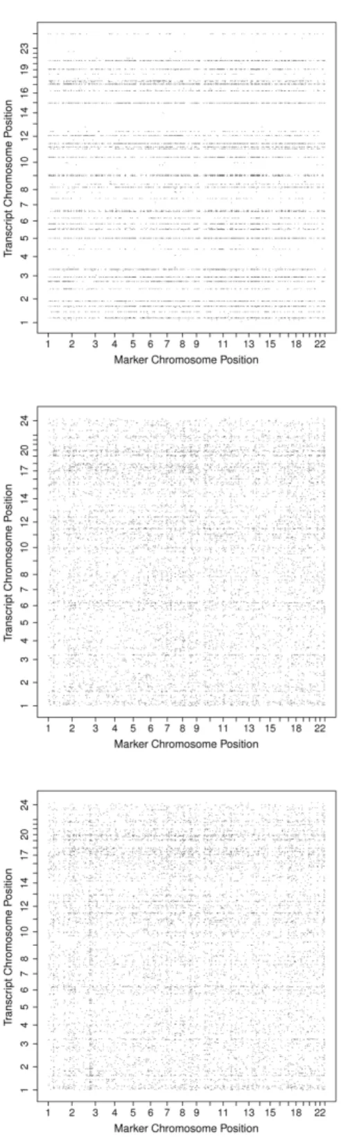
2.3 eQTL results of the Human from the raw data (top panel), from the trans-formed data (middle panel) and from the transtrans-formed and adjusted data

(bot-tom panel) . . . 36

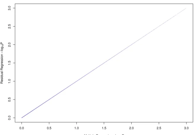
2.4 Results from the residuals compared to the full model of Yeast . . . 38

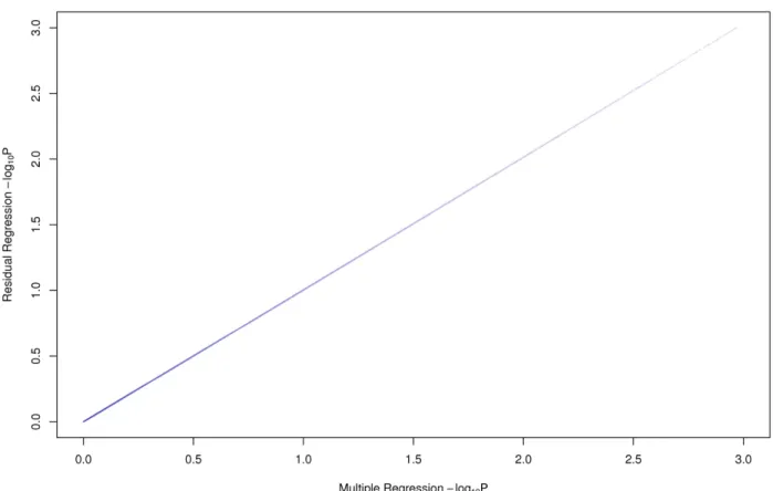
2.5 Results from the residuals compared to the full model of Mouse . . . 39

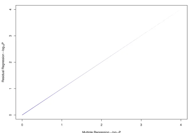
2.6 Results from the residuals compared to the full model of Human . . . 40

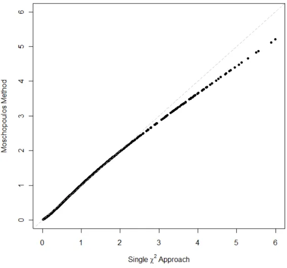
3.1 Comparing the Moschopoulos distribution to the approximateχ2_l . . . 50

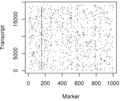
3.2 Randomly permuted marker data mapped analyzed with the true expression data showing random trans bands . . . 53

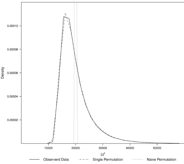
3.3 Densities showing the Σt2 statistics from the true data, under a single permu-tation and under full permupermu-tations or totally permuted data . . . 54

3.4 Results from power simulations with varying effect sizes. The colors represent the ratio of the power between the two methods with red indicating higher power from the continuous sum oft2statistics and blue representing the higher power in the indicator method. Purple shows a greater than 2 fold increase in the indicator method. . . 57

3.5 Distribution of the Σt2 with the approximate fit . . . 58

3.6 Σt2results with the niave, gene covariance, PC method and permutation cutoff for Yeast data . . . 60

(9)

3.8 Σt2results with the niave, gene covariance, PC method and permutation cutoff for Yeast data . . . 63

4.1 Relation between the correlation of the standard and folded normal distribution 74

(10)

List of Tables

1.1 Description of possible outcomes given the underlying truth of multiple hy-potheses . . . 14

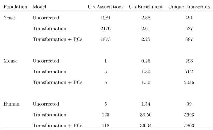
2.1 Characteristics of the significant associations in each model for each organism 32

3.1 Thresholds obtained from the various methods using theP

t2 statistics . . . 60

3.2 Thresholds obtained from the score statistic method . . . 61

4.1 Significance thresholds produced by each method . . . 82

4.2 Expected number and permuted number of clumps under the null distribution for the yeast data . . . 85

4.3 Expected number and permuted number of clumps under the null distribution for the human data . . . 86

4.4 Describing the FDR in terms of clumps for 5 known true associations using the yeast data . . . 88

(11)

Chapter 1 Introduction

Two popular methods of genetic experimentation and analysis are microarray gene expression

studies and marker associations studies. The first design focuses on gene expression profiling

and the second design is used to identify single nucleotide variation. Each type of experiment

addresses a different biological phenomenon, and both designs were initially performed and

analyzed independently. Gene expression experiments and polymorphism association

experi-ments generate large amounts of data that require different methods of analysis. The amount

of data created by each experiment is in part why results were not initially combined as it

requires both large amounts of digital storage and processing capabilities. Analytic

com-plications also increase with the addition of more data. Gene expression analysis and SNP

genotyping each have unique analytic methods that employ different assumptions about the

data. Similarities between the analytic methods do exist, but with each experimental design

having different goals of discovery, the similarities are limited. Recently, methods have been

described in which the data from both gene expression and SNP genotyping data can be

analyzed together. This combination of methods is known as expression quantitative trait

analysis (eQTL). The design of eQTL experiments is relatively new in the genetic literature

and has adopted most of the methodology from the previous gene expression and SNP

geno-typing studies. In describing the specific eQTL analytic methods, we will begin with taking

(12)

1.1 Microarray Studies

The name microarray refers to the technology used to analyze the genetic samples. A

mi-croarray is a chip that is used to measure the expression activity of thousands to tens of

thousands of genes simultaneously. The expression of an individual gene is measured by one

or more probes located at known spots on the array. Samples are fluorescently tagged and

applied to the array. Light intensity is then recorded from each spot on the array. Each

Gene expression microarray analysis begins with the normalization of the array values. Some

subject’s samples tend to bind more effectively to probes regardless of their level of expression

which can cause a bias in the analytic methods. Several types of normalization methods exist

which make selection of a particular method dependent on the goal of the analysis. Popular

methods of normalization include median or mean centering, ranking and logarithmic

trans-formations (Wit and McClure, 2004). Once normalization has been performed, the primary

analysis can be carried out.

Simple microarray studies involve only the transcript intensity levels recorded from the

plates. More complicated designs employ the use of dependent, phenotypic values that are

measured independently of the transcript expression procedure. The high dimensionality

at-tribute of the data make them appealing for classification and pattern recognition analytic

techniques. Clustering algorithms offer quick and easy solutions to analyzing the high

di-mensional data and are able to perform in situations where the number of responses greatly

outnumbers the number of subjects. Hierarchical clustering is often the standard algorithm

applied when clustering is performed however k-nearest neighbors and Gaussian mixture

models are often popular alternatives. Additional classification methods similar to clustering

analysis are also often applied to microarray data and include support vector machines,

pre-diction analysis microarray (PAM) (Mukherjee et al., 1999; Tibshirani et al., 2002), decision

tress and random forests (Slonim, 2002). Use of a dependent variable in microarray studies

requires a different set of analytic tools. The simplest example of microarray studies involving

(13)

compared to one another. With a binary outcome, the goal of the analytic model is to

de-tect differential expression between the two groups of cell responses. Case-control microarray

analysis can be easily carried out using standard t-tests given the responses meet the

assump-tion criteria of the t-test. Significance analysis microarrays (SAM) (Tusher, Tibshirani and

Chu, 2008), Wilcoxon tests and other non parametric methods, ANCOVA, logistic regression

and Bayesian t-tests all represent popular alternative methods for detecting differential

ex-pression. Linear and generalized linear models are techniques that allow the statistician to

account for additional covariates in the model that may improve power in detecting

differ-ential expression. Additional predictors can include environmental or clinical measures that

when adjusted for can help improve the variability accounted for by the model. Mixed effects

models have also helped control within cluster variability during the fitting procedures.

Given the design and methods on which microarray experiments are carried out, several

known issues arise when assessing the reliability of the data. Outliers in the data can be

caused by florescent dust present on the array or neighboring spots can influence the reading

of one another (Nadon and Shoemaker, 2002). The outliers can affect the statistical inference

and lead to inaccurate conclusions based on the data. Binding of the cDNA to the probes can

also cause inaccuracies in the data. Samples may fold upon themselves and thus be unable to

bind to the probes on the array(Zhang et al., 2005). Other issues arise are when the samples

may bind with the wrong probes because of a similarity of the probe and sample strand (Mir

and Southern, 1999). Each individual sample may also contain variants and so binding may

not completely occur with the probe. The true relationship between the probe and sample

is not always understood in that certain probes have better chances at binding with samples

(Draghici et al., 2006). Even samples with variants that don’t match the probe completely

can create higher intensity values than those that match completely to the probe (Sugimoto,

Nakano and Nakano, 2000; Naef and Magnasco, 2003). These previously identified issues as

well as environmental interference can cause the data from microarray experiments to have

inaccurate results. Normalization of the data can help alleviate some of the extra variation

induced by these problems but can not correct for everything.

(14)

difficult to obtain because of biologic issues. Often the reproducibility of different platforms

relies on the original design of the probes and how likely they are to succumb to the influences

described above (Draghici et al., 2006). For these reasons, any analysis of microarray data

should try to limit the influence of any individual observation due to its potential bias.

1.2 Association Studies

Genotyping studies suffer the same design issues as in gene expression analyses, mainly that

the number of observations per subject often greatly exceeds the number of subjects being

analyzed. Analysis of the genotype data alone does not offer the same advantages as the

analysis of gene expression data. The primary analysis of genotype data involves identification

of a phenotypic association with a particular locus. Often these associations are indirect

associations in that the significant locus is correlated with a second unobserved locus that

is the true biological cause on the dependent phenotype (Balding, 2006). The mechanism

behind indirect association is known as linkage disequilibrium. Linkage disequilibrium is

when markers show an association with one another which happens more than expected by

chance. Linkage disequilibrium can be caused by the absence of recombination hotspots

between the markers. Indirect association can lead to a decrease in effect size for a particular

discovery which in turn can lead to a decrease in power and increase in required sample size.

Most analytic methods resemble univariate techniques that identify an association between

genotype information at a given locus with the dependent phenotype. Association methods

include standard models such as linear or logistic regression and chi square analysis as well

as more genetic based models like transmission disequilibrium tests. Most analytic methods

assume all the markers are independent. For markers separated by great distances this is

not an unreasonable assumption however, markers that are located near one another on the

genome likely have some measure of correlation between them. For this reason treating all

tests as independent can reduce the power of the analysis.

Once an analysis population is identified and genotyping platform is selected, the samples

(15)

are a number of methods to detect and remove errors found in the genotyping data. The

genotyping platforms also rely on intensity measures and thus markers that produce consistent

low intensities in the sample should be removed. The call rate, rate at which an individual

SNP is identified across the population, can also be used for quality control. Call rates less

than 95% are often considered less than optimal markers (Draghici et al., 2006). The call rate

for an individual is also useful for quality control. Individuals with more than 20% missing

data are useually removed from analysis (Draghici et al., 2006). Markers with calculated low

minor allele frequencies will most likely not be useful for analysis and are often removed. For

studies involving populations that undergo random mating, alleles are expected to maintain

certain distributions. Departure from Hardy-Weinburg equilibrium can be tested using the

distriubtion of the marker data.

Population stratification is a more complex issue rooted in genotype association

stud-ies. Populations are likely to show different patterns of variability throughout the genome

(Consortium, 2005). In some populations a particular marker may show no variability in the

population being analyzed and therefore not provide any useful information to the analysis.

Isolated genetic populations can cause a difference in allele frequency at a specific locus due

to selective mating. Any experiment that combines multiple populations can be subject to

spurious results caused by population stratification. It has been shown that latent

stratifica-tion can also exist within a populastratifica-tion that is not easily detected by quesstratifica-tionnaire or other

phenotypic data. Latent stratification can also cause spurious association with the phenotypic

outcome of interest (Campbell et al., 2005). Methods like principal components analysis and

mixture models which use genotypic information can address the population stratification

(Paschou et al., 2007; Price et al., 2006). Using simple demographic covariates can be

unre-liable and overly simplistic in assessing population stratification and normally are only able

to detect the highest degrees of stratification. Principal components and mixture models are

(16)

1.3 eQTL Studies

Early eQTL studies focused on model organisms with well described genomes. The aims of the

analysis were to identify associations between transcripts and markers and potentially identify

larger patterns in the data. The organisms first analyzed include yeast, arabidopsis, and maize

(Brem et al., 2002; West et al., 2007; Schadt et al., 2003). Analytic methods employed in

these initial studies were often simple statistical procedures without the aid of adjustments or

transformation. Early analysis procedures often evaluated every pairwise association between

the gene expression transcripts and polymorphic markers using a correlation type measure,

Wilcoxon test or other simple test statistic. Results from these test statistics were used to

identify patterns across the genome of the organism being studied. Initially two different

types of associations were described in eQTL studies. The first type of association is between

polymorphisms and transcripts that lie within short distances of one another on the genome.

These associations where the two points lie in close proximity are known as local associations

or cis associations. The second type of association is where the marker is located away

from the transcript. This second type of association is known as distant association or trans

association. The two types of associations were first described in eQTL studies by Brem et

al. (Brem et al., 2002). Brem et al.were also first to describe the regions that produced

more trans associations than were expected by chance. It was Schadt et al. in 2003 (Schadt

et al., 2003) that first named these regions hotspots. Both Brem and Schadt also showed

that cis associations were often more statistically significant than trans associations. As

previously mentioned, these initial studies carried out simple analytic techniques to evaluate

the associations.

As mentioned the first eQTL studies relied on simple statistical procedures to evaluate

each transcript with each polymorphism. More complex procedures have been proposed which

incorporate multiple markers or transcripts in each model. A Bayesian approach was proposed

by Kendziorski et al. (Kendziorski et al., 2006) which aims to share information across both

the markers and the transcripts. Kendziorski’s method is known as Mixture Over Markers

(17)

given marker. The MOM method employs K-means clustering to identify transcripts with

similar variabilities.

f0(yt) =

Z n Y

k=1

fobs(yk,t|µ)

π(µ)dµ (1.1)

In the equation fobs(yt,k|µt, σ2) = φ(yt,k;µt, σ2) and π(µt) = φ(µt;µ0, τ02). It is the σ2

pa-rameter that is held cluster dependent and not constant. The Bayesian approach calculates

posterior probabilities incorporating information across all transcripts which identify an

as-sociated marker. A second Bayesian approach was proposed by Jia et al. which attempts to

simultaneously evaluate the entire set of marker loci (Jia and Xu, 2007). Their method uses

Bayesian shrinkage which shrinks markers with smaller effects to zero but does not adjust

markers with larger effects. This procedure is carried out using hierarchical Gaussian mixture

models and estimates the parameters through a sequence of MCMC samples. Jia’s method

differs from Kendziorski in that MOM allows transcripts to be identified with at most one

marker, whereas the Gaussian mixture models allow for a given transcript to be associated

with multiple markers. A similar procedure using mixture models has also been proposed.

The use of mixed models was employed by Kang (Kang, Ye and Eskin, 2008) to estimate

variance components. This mixed model method allows for easily testing hypotheses on the

parameter estimates. Mixed models also allow for the easy addition of data to the model by

means of covariates.

As with association studies, haplotypes can be used in eQTL studies to define regions

of high correlation with several markers. A unique haplotype approach was developed by

Pletcher et al.(Pletcher et al., 2004). Their method uses 3 SNP sliding window haplotypes

instead of the single marker association test. The use of an ancestral haplotype to identify

associations is proposed to have more power than the standard one marker association test.

The sliding haplotype approach was further developed and implemented in other mouse

stud-ies (McClurg et al., 2006, 2007). In their 2006 study, the researchers identified the optimal

(18)

evaluate associations and limiting false discoveries. In their 2007 study, the researchers

em-ployed the sliding window approach on a diverse mouse population containing both wild and

lab strains. The diversity of the population and limited sample size provided the need for

further refinement to their method which was solved by a unique bootstrap style permutation

test used to control spurious associations.

Other more sophisticated methods have also been developed in the literature. Some

ap-proaches have been made to reduce the number of statistical tests by grouping the gene

expression transcripts. Lan et al. proposed the use of principal components and

hierarchi-cal clustering to analyze the expression data separately from the marker data (Lan et al.,

2003). Both principal components and hierarchical clustering attempt to reduce the high

dimensionality of the expression data. Principal components reduces the data by extracting

the different axises of variance, whereas clustering relies on differences in response distances

between the genes. Both methods can effectively reduce the high dimensionality and produce

smaller numbers of grouped genes. Biswas et al. proposed a similar technique in which they

use singular value decomposition to reduce gene expression dimensionality (Biswas, Storey

and Akey, 2008). The singular value decomposition method also reduces the number of

tests by identifying associations with larger groups of genes reduced into single components.

Perez-Encisco et al. also attempted to reduce the number of tests using partial least squares

techniques (P´erez-Enciso et al., 2003). Their approach assumes an underlaying relation

be-tween the expression values. They employ the partial least squares regression to target genes

with stronger association to the markers. Similar reduction techniques have been proposed

by other authors.

A networking method using correlations between gene expressions was proposed by Chesler

et al. (Chesler et al., 2005). The researchers used graphical techniques to uncover networks of

transcripts in gene expression data. The basis for this method is that the false positive rate is

lower for genes with high gene by gene correlation. The researchers defined the term ’cliques’

to describe highly associative networks of genes defined by the transcript data. It is proposed

that these cliques can uncover the molecular processes in which some of the transcription

(19)

is thought of as a genetic marker directly or indirectly controlling a large amount of transcripts

throughout the genome without specifying the relationship between the transcripts. A clique

on the other hand explores the correlation between transcripts and identifies markers with

one or more associations to members of the clique.

Drawing from the idea of a clique, Huang developed a method which relies on networks

identified by correlation to remove improbable associations thereby lowering the false positive

rate (Huang et al., 2009). The graph theory methods rely on specifying the direction of the

transcript regulation, the genotype allele and the particular strain. By modeling this in a

graph, disjoint subgraphs can be extracted in which the number of associations is limited to

relationships that are more likely to exist. This method cuts down on potential false positives

by eliminating the possibility of many interactions.

The enrichment of cis associations have been used as a standard in evaluating the reliability

of the results for eQTL studies (Brem et al., 2002; Schadt et al., 2003; McClurg et al., 2007;

Stranger et al., 2007a). Even though cis associations are more understood and plausible

associations, the set of cis associations can contain false positives. Doss et al. brought some

attention to the idea when they were unable to to confirm some of the cis association previously

reported in mice through quantitative RT-PCR and that local associations are not always true

cis associations. The investigators discussed the idea that marker variants overlapping probe

regions could cause false positive results due to incomplete binding of the probes. This idea

of incomplete binding was brought up again by Alberts et al. (Alberts et al., 2005). Their

study of mice showed two specific markers that caused differential hybridization with the

expression probes when analyzed. The investigators proposed the use of a model in which to

better discern probe specific cis associations, which are more likely differential hybridization,

and broad panel cis associations, which are more likely to be biologically relevant.

log(yij) = m+Bi+Pj+P Bij+Ai+P Aij+ei+eij (1.2)

Their model estimates interaction terms for probe by batch (P Bij) and probe by gene

(20)

developed the model on mice and humans in a follow up study (Alberts et al., 2007). For

the human data, they removed the batch parameters in their original model (Bi, P Bij) , but

are still able to detect differences between cis associations caused by differential hybridization

and those more likely to be true regulatory associations.

Identification of individual marker/transcript associations does provide some information

about the relationships between alleles and expression but can often be difficult to

inter-pret. The vast amount of significant results when investigated individually may not provide

a picture of the overall relationships in the total experiment. The relevance and role of a

single marker/transcript interaction is unclear when examining the associations individually.

Grouping associations can provide better information about an overall process or discovery

but determining groupings can also be an arbitrary exercise. A popular grouping of the

asso-ciations that can provide information about larger interactions and networks are trans bands

or eQTL hotspots. These classifications can allow investigators to arrange the significant

associations into potential larger networks that offer a better overall idea of the experiment.

1.4 Trans Band Analysis

As mentioned earlier, trans bands or eQTL hotspots are of great interest to investigators. The

simple definition of a hotspot is a region on the genome that has more transcripts associated

in trans than expected to occur by chance (Schadt et al., 2003). To determine the expected

number of QTL associations per region, the genome was divided up into equally spaced bins of

some genetic length. Then the total number of significant QTLs was divided by the number of

bins giving an average expected number of QTLs per bin. Assuming this distribution follows

a Poisson distribution with the same mean, significance thresholds could be calculated that

identify hotspots. Other studies that have similar approaches include Morley (Morley et al.,

2004) and Duan (Duan et al., 2008). Both Morley and Duan studied human eQTL data

and used similar bin distribution methods to identify potential hotspots. This approach of

creating equal bins has been challenged first by Darvasi (Darvasi, 2003) and Perez-Encisco

(21)

between sets of genes, the resulting hotspots could be falsely inflated. Both Darvasi and

Perez-Encisco pointed out that high rate of false positives due to the large amount statistical

tests being performed could also inflate these hotspots. Many other different tests have been

proposed to evaluate the significance of hotspots.

Kendziorski et. al identified eQTL hotspots by summing their test statistics over each

marker (Kendziorski et al., 2006). They then looked at the maximum sums as evidence of

hotspots, but provided no significance threshold. Similar results were presented by Bystrykh

(Bystrykh et al., 2005) and Chesler (Chesler et al., 2005). Both authors reported on mice

populations and investigated regions that had abnormally high trans associations. These

bands were often further explored in which some biologic mechanism was suggested as the

source of the apparent genetic control.

A more sophisticated approach was developed by Peng (Peng, Wang and Tang, 2007) using

elastic net regression techniques. They proposed several regression models to test whether

trans association between a given marker was direct or indirect. Once the direct linkage

associations were determined, an elastic net model was fit which minimizes the loss function

L(λ1, λ2, β) = ||Y −Xβ||22+λ2||β||22+λ1||β||1 (1.3)

This loss function favors the grouping of strongly correlated terms with the penalty term.

The parametric setting of their method allows for testing specific hypothesis and determining

thresholds for their analysis.

A widely used approach to determining the significance of eQTL hotspots is the use of

permutation testing. Early eQTL studies limited the use of permutation testing because of

the computational time it demands. When analyzing mouse eQTL data, Kang (Kang, Ye

and Eskin, 2008) used the average of the log p-values across all probes as a measure of trans

activity. They performed 10,000 permutations of the SNP data to determine significance

thresholds for trans hotspots. A different permutation approach was used by Wu et al. (Wu

et al., 2008) in the analysis of mice. They analyzed the data using the 3 SNP haplotype

(22)

bands in the data. They performed permutations by randomly selecting SNPs from a subset

of markers that had at least one association and then performed permutations on the given

gene. This approach requires less markers than full permutation procedures but the chance

of observing a significant association is higher by definition of the subset.

Different permutation procedures than Wu’s have been developed that keep the expression

data unchanged. The reasoning behind this is that the correlation between transcripts could

be mechanism behind some of the trans bands and therefore should not be removed when

determining a threshold. One study to apply this method was presented by Li et al. (Li

et al., 2006). Their method permutes the genotypes but do not alter the structure of the gene

expression data. This allows for correlation that exist between transcripts to be acknowledged

when computing thresholds for markers. Their method does remove the correlation structures

present in the markers. Following a similar approach, Breitling proposed a permutation in

which the strain labels of the marker data are permuted and the gene expression data are

kept constant (Breitling et al., 2008). Again this method allows for the impact of transcript

correlation structures as well as between marker correlation structures. Breitling also lists

a number of previous studies, their reported thresholds and number of hotspots discovered.

An interesting find is that the threshold varies greatly between and within organisms. The

thresholds from the literature review changed between both the population size and organism,

but even studies performed on the same organism with similar sample sizes produced different

thresholds and different numbers of hotspots.

It has been proposed that eQTL hotspots are the results of master regulatory markers. Yu

and Li proposed a method to identify transcription factor activity within microarray studies

(Yu and Li, 2005). Their method identifies transcript factor genes that exhibit control on

other genes on the array. Using this methodology developed for the microarray experiment,

Sun et al.extended the methods to the eQTL setting (Sun, Yu and Li, 2007). They developed

a number of directional models to account for markers that control transcription factor genes

that control other genes expression on the array. They hypothesized that the intermediate

transcription factor gene related to trans markers is the underlying cause for eQTL hotspots.

(23)

and gene product interactions to explain the eQTL trans associations. One such resource,

Gene Ontology (GO) (Ashburner et al., 2000), provides groupings of gene interactions with

associated biological processes. Yvert used GO databases (Yvert et al., 2003) to attempt

to describe the trans bands found in yeast. They found no significant enrichment of any

biologic function in the resulting trans associations. They specifically targeted a subset of

molecular functional categories known for yeast. On a study of mice, Lan employed the use

of GO terms by exploring the correlation of their expression data (Lan et al., 2006). They

looked for evidence of enrichment for any GO term between from a subset of transcripts

that showed high correlation with at least one marker. Enrichment analysis was carried out

using hypergeometric distributions. Another mouse study to use GO terms was done by Wu

(Wu et al., 2008) which has been previously discussed. Wu also used the hypergeometric

distribution to carry out tests on the enrichment of GO categories.

Storey et al. proposed a more complex model to identify different regulatory networks

(Storey et al., 2005). They proposed modeling multiple markers in a single model with

the potential of interaction terms. In their manuscript they explored only two loci in a

single model with the interaction term in a multiple regression model. This model allows for

evaluating epistasis between two loci at a time. To reduce the number of all pairwise locus

tests, Storey et al. propose the use of a stepwise selection technique. This technique uses a

Bayesian approach conditioning on the association of a previously linked locus. This stepwise

selection is particularly useful in models that include more than two loci.

The biological mechanisms behind trans bands are not fully understood (Perez-Enciso,

2004). For this reason, developing a method that can accurately designate spurious trans

bands from relevant bands has not been universally accepted. Even without the underlying

truth known to the researcher, some clues present in the data may help to determine bands

or hotspots that are more likely due to the structure of the data and not some biologic

phenomena. Use of dependence structures is crucial in identifying regions that are driven

by the data and can be useful in determining the threshold at which trans bands should be

considered of interest or significant. Most of the methods previously discussed make use of

(24)

is important to consider the impact of both these dependence structures and how they might

influence the appearance of trans bands.

1.5 Multiple Testing

eQTL and other genetic experiments carry out an abundance of hypothesis tests in each

experiment. Using a traditional threshold in eQTL types of analysis will lead to a meaningful

amount of false positives. The occurrence of many false positives is a result of the correlation

between markers and correlation between transcripts. To reduce the number of false positives

in the results, numerous methods exist to determine more appropriate significance thresholds

based on the size of the data as well as correlation structures that may be present. The

different correction methods fall into either single stage methods or multiple stage methods.

In the single stage methods, the rejection/acceptance of each individual hypothesis is made

based on an individual test. In multi stage methods, the decision about each test is made with

information from the other tests (Shaffer, 1995). In the next pages we will discuss methods

that are applicable to genomic and eQTL studies.

The family wise error rate (FWER) is a mechanism to determine the significance of

indi-vidual hypothesis tests. The term ’Family’ refers to all tests being considered a priori. We will

refer to this value as ’m’ in the coming discussions. If the underlying truth of each hypothesis

was known, the number of correct and incorrect determinations could be organized in a 2 by

2 table (Table 1.1).

Table 1.1: Description of possible outcomes given the underlying truth of multiple hypotheses Accept Reject Total

Null True U V m0

Alternative True T S m1

W R m

In Table 1.1, the value V refers to the number of hypotheses that are declared alternative

but are actually truly null. The probability of at least one hypothesis being falsely declared

alternative, P(V ≥ 1), is known as the family wise error rate (Shaffer, 1995). Multiple

(25)

1.5.1 Single Stage Methods

Adjusting the significance threshold α can create a more conservative threshold for

declar-ing results significant. This type of approach allows the researcher to declare certain results

significant with confidence even after carrying out multiple hypothesis tests. Permutation

testing is considered the gold standard in adjusting the significance threshold α (Churchill

and Doerge, 1994). Permutation testing was introduced in 1935 by RA Fisher (Fisher, 1935).

In its earliest applications, the amount of observations was limited and enumerating all

per-mutations was possible. This approach is commonly referred to the Fisher exact test. The

exact test defines the probability of the test based on permutations created from the observed

data. More recent sources have discussed the use of permutation testing in genomic studies as

a method of controlling the issues that arise with multiple hypothesis situations (Edgington,

1995; Good, 2005). In genetics, the amount of data often prevents the full enumeration of

the data, however generating large amounts of permutations of the data can offer a close

approximation of the underlying probabilities. Increasing the amount of data increases the

required amount of permutations to acquire consistent estimators of the probability.

Resampling techniques are similar to the permutation testing but resampling attempts to

preserve the correlation structures to the data. The most well known strategy, the Bootstap

(Efron and Tibshirani, 1998; Westfall and Young, 1993), is a resampling based procedure used

to generate empirical thresholds by continually drawing samples from the data. Allowing the

resampling attempts to preserve the dependency in the data but can not always be guaranteed

to produce conservative estimates. Producing anti-conservative estimates has the consequence

of no longer offering reliable control of multiple testing outright but still allows for asymptotic

control.

A well known group of correction methods is derived from Boole’s inequality. The

in-equality states for a countable set of eventsA1, A2, . . . then

P [

i

Ai

≤X

i

P(Ai) (1.4)

(26)

with probability p, then α ≤ np or p = α/n. This is known as the Bonferroni correction

and is used to correct for multiple hypothesis tests at level α. A similar method to the

Bonferroni is the ˜Sid´ak correction. The ˜Sid´ak correction assumes that the hypothesis tests

are independent and is obtained using the following equation

p = 1−(1−α)1/n (1.5)

Rarely are hypothesis tests independent from one another in a total set, but the ˜Sidak´ method

can act as a conservative bound for multiple testing correction.

One method of correcting for multiple comparisons focuses on identifying the effective

number of tests. Cheverud proposed estimating the number of effective tests,mef f, by using

the spectral decomposition of a correlation matrix (Cheverud, 2001). This idea stems from the

fact that the collective correlation of a number of variables can be estimated by the variance

of the eigenvalues. The variance is used as a way to reduce the total number of effective tests.

Mef f = 1 + (M−1)

1−V ar(λobs)

M

(1.6)

V ar(λobs) = M

X

i=1

(λi−1)2

(M−1) (1.7)

In the equation M is the number of total tests and λobs are the eigenvalues of the linkage

disequilibrium matrix. Cheverud proposed use of the Pearson correlation between markers in

a QTL study. Using this newMef f, the significance threshold is determined with the ˜Sid´ak

correction. In the ˜Sid´ak procedure, Mef f represents the total number of independent tests

for the total of M tests. Nyholt later modified the method by using other correlation measures

between markers for genome wide association studies (Nyholt, 2004). Nyholt proposed the

linkage disequilibrium matrix as the correlation to compute the eigenvalues. The proposed

modification performed closely to permutation testing however in a significant reduction of

computation time.

A different approach was presented by Moskvina and Schmidt similar to the Cheverud

(27)

that relies on pairwise Pearson correlations. The method has a simpler form that arises for

small levels of α, (α ≤ 0.01), which avoids complex integrations involving the cumulative

normal density. The simple form of their equation is given below.

Kef f1 + M

X

j=2

q

1−r_k−1.31log10α (1.8)

In this formula,rj = max1≤k≤j−1|rkj|, is the largest absolute pairwise correlation between the

jth and preceding markers. The authors also offer a simple approximation to the Cheverud

method which can be used in situations with larger numbers of markers.

Mef f = 1 + 1

M

X

j=1

MX

k=1

M(1−r2_jk) (1.9)

For large enough M values (which are common in current technology), trying to evaluate

the principal components for correlation matrices can be computationally intensive and this

proposed estimate can be used to reduce the computational time.

Li and Ji proposed a different estimate of Mef f from Cheverud and Nyholt’s methods

(Li and Ji, 2005). They noted that the previous two methods overestimated the Mef f and

therefore producing too high of a significance threshold. In developing the previous method,

Cheverud noted the two extremes of correlation with all markers being independent and all

makers being identical. However Li and Ji note that some markers are identical and some

are only partially correlated. Their method breaks the eigenvalues into two portions, those

completely correlated and those partially correlated.

Mef f = M

X

i=1

f(|λi|) (1.10)

f(x) = I(x≥1) + (x− bxc), x >0 (1.11)

The indicator function contains the completely correlated eigenvalues and the second term is

responsible for the partially correlated terms.

(28)

subdivisions and more driven by the data (Galwey, 2009). Galwey also notes that more

weight is given to the partially correlated terms which leads to an overestimate in Li and Ji’s

method. Galwey’s proposed estimate is as follows.

Mef f =

PM i=1

√

λi

PM

i=1λi

(1.12)

Galwey then uses the estimated Mef f in both the Sidak correction and the Fisher method

to obtain significance thresholds for correlated markers. Galwey uses permutation testing to

verify the results of his formula.

Lin proposed a method which utilizes MCMC simulations to estimate parameters for

an observed dataset (Lin, 2005). Modified score statistics are distributed as multivariate

normal random variables which can be accurately simulated using MCMC methods. Using

the MCMC samples to estimate the conditional joint distribution of test statistics, parameter

estimates can be obtained for the unconditional observed statistics. This method is powerful

in estimating significance thresholds for varying degrees of linkage disequilibrium in the data

using the multivariate normal covariance structures.

Other methods focus on the block correlation structures between markers. Conneely and

Boehnke proposed a method that uses the multivariate normal distribution (Conneely and

Boehnke, 2007). Their method assumes that groups of markers follow multivariate normal

distributions with described correlation matrices. For example a block of two markers would

follow a bivariate normal distribution with ρ as the correlation between the two markers.

Then using the multivariate normal distribution PACT = 1−P[max(|Z1|,|Z2|, . . . ,|ZL|) <

Φ−1 1−Pmin

2

]. The difficulty in implementation is that most available software packages can

only handle multivariate normal distributions of dimension up to 1,000. To circumvent this

issue, the authors suggest dividing the markers into independent blocks of correlated markers.

A similar type of approach was proposed by Duggal et al. (Duggal et al., 2008). They

use the the Haploview software package (Barrett et al., 2005) to estimate blocks of linkage

disequilibrium. These blocks are defined by an LD threshold of 0.7 or 0.8, which estimate the

(29)

the number of markers between blocks. Both the multivariate normal method and Haploview

method require the genome to be divided into independent blocks. While this may be true of

markers on different chromosomes, it is unlikely that the blocks within the same chromosome

are completely independent. Han et al. makes this observation in developing their SLIDE

method (Han, Kang and Eskin, 2009). The SLIDE approach also assumes a multivariate

normal distribution for describing the relationship between markers. The authors also assume

independence between blocks but allow their algorithm to naturally estimate the blocks.

Instead on relying on a series of independent multivariate normal distributions, they propose

a single multivariate distribution of dimension M, where M is the total number of markers. The

method estimates the joint distribution by using the product of conditional distributions. The

full method further adjusts the multivariate normal distributions by scaling them according

to MCMC simulations. Another normal distribution method is Direct Simulation Approach

(DSA) proposed by Seaman and Muller-Myhsok (Seaman and M¨uller-Myhsok, 2005). The

DSA method uses the vector of individual score statistics generated by each marker. The

variability of these score statistics is also calculated from data. Under the null distribution the

score statistics follow aN(0,V) distribution where the variability is that of the score statistics.

By knowing the distribution, permutation samples can be generated rapidly. Additionally

for subsets of markers, the conditional variability can be calculated rapidly as well using

conditional normal distributions without having to estimate large variance matrices. The

authors also assume that markers separated by large distances are independent.

Distributions other than the multivariate normal distribution have also been proposed.

Dudbridge and Koeleman proposed the use of two different distributions depending on whether

fixed or variable window lengths are assumed (Dudbridge and Koeleman, 2004). First for fixed

window sizes an extreme value distribution is assumed for the marker dataset. The extreme

value distribution contains parameters for location, scale and shape. Likelihood fitting

esti-mates the location parameter proportional to the total number of markers conditional on the

size of the block. The scale parameter is proportional to the block size conditional on the

total number of markers. Finally the shape parameter summarizes the correlation structure.

(30)

distribution is used to estimate the distribution of the smallest p values. Different lengths are

fitted to obtain a maximum likelihood when the block size is unknown. The second parameter

from the beta distribution is equivalent to the effective number of tests by use of likelihood

ratio testing.

1.5.2 Multi Stage Methods

Popular types of multi stage methods are step up or step down methods in which the p

values are ordered from smallest to largest. Each step produces a different threshold and the

rejection of each p value is dependent on the rejection status of other hypotheses. One simple

multi stage method is one that is constructed from the Bonferroni method. Holm proposed a

sequential correction method based on the Bonferroni correction in 1979 (Holm, 1979). The

sequential procedure begins with the ordered list of p values and starting with the smallest

p value rejects if p(i) < α/(n−# rejected in p(j)) j < i. The proposed sequential method

is more powerful than the ordinary Bonferroni method. At each step a p value is compared

to a threshold but the threshold is based off of how many hypotheses have been previously

rejected. Since each hypothesis tests relies on information from other tests, we can not select

a single p value knowing only the length of the list and determine whether it is rejected or

not. We must have information about all p values smaller than one selected to determine the

threshold.

One widely used method was proposed by Benjamini and Hochberg in 1995 (Benjamini

and Hochberg, 1995) to control the false discovery rate (FDR) and in turn weakly control

family wise error rate. The false discovery rate can be defined as the number of false positives

over the total number of rejected hypotheses. Since this is an unobserved random variable,

then Benjamini and Hochberg propose using

E

V R

(1.13)

to control the false discovery rate and thus weakly control the family wise error rate. They

(31)

Simply put the algorithm orders the p values from smallest to largest. For the p values

p(1) ≤p(2) ≤ · · · ≤p(m) from corresponding hypotheses H(1) ≤H(2)≤ · · · ≤H(m) find ksuch

that

k = max

i:p₍_i₎≤ i

mq (1.14)

then reject H₍₁₎0 . . . H₍0_k₎ and reject no hypotheses for the case when k = 0. This procedure

controls the false discovery rate at the level q∗ where

q∗ = arg min

i≤k{q :i/m∗q ≤P(i)} (1.15)

The authors qualify the method in that it is designed to work in settings where the p values

are nearly independent. This procedure was later shown to hold for certain dependency

situations and a further modification was introduced to maintain control in situations with

arbitrary dependencies (Benjamini and Yekutieli, 2001). By replacing q in the inequality by

q

Pm i=11i

, the procedure is now able to control for arbitrary dependency in the data. For zero

rejected hypotheses, the false discovery rate equals the family wise error rate and thus has

week control of the family wise error rate.

Building from the resampling methods and controlling the false discovery rate, Yekutieli

and Benjamini proposed a resampling based false discovery rate control method (Yekutieli and

Benjamini, 1999). Their method was designed to work in situations with arbitrary dependence

structures without being specified. Using resampled data, a null distribution and alternative

distribution of the p values can be constructed. From knowledge of the null distribution of p

values, quantiles can be used in identifying thresholds to control the false discovery rate.

The advantage of the false discovery rate procedures is that information about the

corre-lation between tests is not required and that they can be performed with a list of available

p values. However by not incorporating the dependency of the data, each test is considered

an independent discovery. If two tests were highly correlated, current FDR procedures could

(32)

the best interest of the researcher to declare multiple instances of the same phenomena as

truly unique discoveries. The effective number of hypotheses techniques attempt to use the

dependency of the data in an attempt to describe the actual number of independent events

but offer no easy method of determining which tests are truly related or are unique discoveries.

Storey and Tibshirani proposed an improvement to the false discovery rate that conditions

on having positive findings (Storey and Tibshirani, 2001; Storey, 2002, 2003). Their method

is designed to work in settings where the probability of making no discoveries is high. The

Benjamini and Hochberg false discovery rate is defined as

E

V R

R >0

P(R >0) (1.16)

Storey and Tibshirani propose the following formulation

E

V R

R >0

(1.17)

In their method, they condition onR >0 which makes the method relevant in settings where

there are positive findings. The pFDR uses the optimal estimate of the ratio of false positives

out of the total number rejected to the fit the rejection region. The formula for estimating

the pFDR for a rejection region [0, γ] is

pF DRˆ λ(γ) =

ˆ

π0γ ˆ

P r(P ≤γ){1−(1−γ)m_} (1.18)

In the formula ˆπ0 = #(pi

≤λ)

(1−λ)m. The method utilizes bootstrapping of the pF DRˆ (γ) to obtain confidence intervals as well as estimates of the mean squared error. Storey and Tibshirani

point out that in situations where no single hypothesis can be rejected are of little interest

to the researcher. The positive False Discovery rate can be described as a Bayesian posterior

type 1 error. This is due to the conditioning on the number of discoveries being larger than

0 and assumes the hypothesisHi are random variables from some underlying distribution.

Another category of testing is Bayesian multiple testing. We will briefly discuss the main

(33)

error or calling a hypothesis alternative when it is actually null (Scott and Berger, 2006). A

loss function can formulated to penalize discoveries that are false positives in the following

manner for calling whereAi is the alternative action and Ni is the null action for hypothesis

Hi for the dataX.

L(Ai) =

    

1 ifHi is null,

0 ifHi is alternative

(1.19)

L(Ni) =

    

0 ifHiis null,

cTi ifHiis alternative

(1.20)

For the loss equation based on the null, the parameter c is adjustable to optimize the loss

functions and Ti represents the test statistic used for the ith hypothesis. After solving the

posterior expected loss for each equation it can be found that E[L(Ai)|X] < E[L(Ni)|X].

Working from this relationship and optimizing the parameter c can allow for the determination

of a p value threshold for significance. The main idea behind the Bayesian approach is that

as long as the expected loss due to false discoveries is bounded by that of the expected loss

from false negatives, then calling a hypothesis alternative is advantageous. More complicated

procedures exist for Bayesian methods and as always specification of a prior hypothesis effects

the expected posterior loss functions. Often Dirchlet related distributions are popular for prior

distributions in dealing with multiple testing scenarios. More details of different Bayesian

methods are available in numerous sources and since our discussions moving forward will not

include Bayesian methods we only wanted to introduce the concept and compare the ideology

(34)

Chapter 2 eQTL pairwise associations

2.1 Introduction

Statistical analysis performed on eQTL data produces a numerous amount of results, more

than that of either microarray studies or association studies. For this reason, any bias or

inconsistency of the data that may be of minimal consequence in a microarray analysis or

marker association analysis can have greater influence on the results in eQTL analysis.

Partic-ular interest must be given to the assumptions used in the models developed to analyze eQTL

experiments to prevent any unwanted consequences to the results. Many of the methods that

have been developed for eQTL analysis were originally designed for either microarray studies

or association studies. When applying these methods to eQTL analysis, certain aspects of the

data are ignored as the method in question was not designed to address all the complications

that arise when performing eQTL analysis. It is important to understand the structure of the

experiment to determine which characteristics could lead to incorrect inference and biased

results. In this chapter we will focus on two major aspects of eQTL experiments that can

lead to biased results if left unaccounted for.

The first issue is the appearance of extreme observations or outliers in the expression data

(Nadon and Shoemaker, 2002). Traditional methods used with expression level data begin

with normalization or ranking. The transcript expression data are often normally distributed

or can readily be transformed. Even after transformations, statistical analysis of experiments

(35)

transcript values in traditional expression level analysis do not have the same level of impact

on the results(Stranger et al., 2007a). This is primarily due to each transcript being analyzed

once and the chance of a single data point being of significant influence is relatively low.

In eQTL analysis, the transcript is analyzed thousands to hundreds of thousands of times

which can lead to a greater proportion of cases where a single data point can have significant

influence on the results.

The next issue is mediation by population substructure. Known population differences as

well as unknown substructures are present in most study populations. Recent literature has

indicated that significant population substructure can exist and cause spurious association

in analysis (Price et al., 2006). Any method used to adjust for the effect of population

differences must be able to handle obvious, usually known dissimilarities between populations

as well as smaller more subtle differences identifiable at the genetic level. Popular methods

of adjustment such as race/ethnic covariate classifications often fail to properly detect the

subtle differences within different ethnic groups. Additionally, self report methods are also

vulnerable to errors in recording, missing information or indetermination.

2.2 Methods

The methods we describe here are designed with relatively few assumptions that are

employ-able on a wide variety of experiments. For the transcript data we assume that each transcript

is normally distributed. Normality is easily obtained in most available analysis and

expres-sion data management software packages. For the marker data, studies that record bi-allelic

markers will use the basic unpaired t-test statistic which can be expressed in the framework of

the linear model. For more detailed records such as the number of alleles at a given position,

an additive effect will be assumed and evaluated using the linear model.

(36)

In the model G represents the vector of individual genotypes taking either values 0 or 1 in

the case of linkage data and can have values of 0,1 or 2 in the case of diploid data.

The effect of extreme observations in the expression data as presented earlier can cause

bias in analysis. Studies with smaller sample sizes are especially vulnerable to the effect of

outlaying observations. To remove the effect of outliers in expression data without removing

observations, we propose the use of Van der Waerden transformations (Van der Waerden,

1952, 1953). The transformation uses the quantiles of the data and the inverse of the normal

quantile function. Fory|r|, therth ordered value ofy,

y0_|_r_| = ψ

r n+ 1

(2.2)

whereψis the inverse of the cumulative normal distribution function. The Van der Waerdern

transformation provides an equal or more powerful result than that of a Wilcoxon signed rank

test(Van der Waerden, 1952). The quantile transformation imposes a normal distribution on

the responses. The normal distribution restricts the variability in the data and reduces the

deviation of the outlying values. Additionally, the expression values now have a distribution

that meets the assumptions of the linear model.

We propose the use of principal components to adjust for the effects of population

sub-structures present in the data. The principal components are calculated from the genetic

marker data of the subjects. Use of principal components has often been employed in single

trait QTL analysis (Paschou et al., 2007; Bauchet et al., 2007; Price et al., 2006) but has

not been seen in the eQTL literature. When compiling the components, several assumptions

about the data must be made to ensure proper description of the populations. Calculations of

the principal components should contain only unrelated individuals as not to bias population

contributions. Imputations can be used to calculate components on the individuals excluded

from the original component calculations and are available in most software packages. The

use of multiple eigenvectors to describe different populations allow for adjustments based on

multiple population layers for each individual. This is an advantage in describing participants

(37)

EIGENSOFT (Price et al., 2006) is proposed to calculate the principal components for

eQTL data. Different approaches exist to determine the appropriate number of eigenvectors

to include in the analysis. The initial naive approach is to select vectors for eigenvalues that

are greater than 1. This method can still result in the selection of too many eigenvectors.

To compute the principal components, EIGENSOFT utilizes the singular value

decompo-sition ofXwhereX is themnucleotides bynindividuals matrix of transcripts. The singular

value decomposition composition provides the following relationship:

X = V DU0 (2.3)

In the expression V is the matrix of orthonormal eigenvectors of XX0, U0 is the matrix of

orthonormal eigenvectors of X0X and D is a diagonal matrix consisting of square roots of

the eigenvalues. Theith row of the jth column of U0 represents the ancestry component of

theithindividual along the jthprincipal component. The vectors representing the principal

components can be used as covariates in the linear model. For populations containing related

individuals or highly correlated clusters of subjects,X can be formed using a unique subset

of the entire population. The resulting V and D matrices can be used as loadings on the

remaining individuals to project their values onto the components and assign them a score.

To further reduce the number of vectors selected, Tracy-Widom statistics can be tested

for significance of each eigenvalue. In studies with smaller sample sizes, the number of

com-ponents is bounded by the degrees of freedom. For our analysis we will identify the number

of eigenvalues to adjust by using the Tracy-Widom statistics. An α = 0.05 will determine

whether or not the statistic is used with a minimum of two components to be included as

ad-ditional covariates in our models. The distribution of the eigenvalues will be presented briefly

below, for a complete description details can be found in Patterson et al. 2006 (Patterson,

(38)

Define the following population rescaling parameters based on the dimensions ofX.

µ₍_n,m₎ = (

√

m−1 +√n)2

m (2.4)

σ(n,m) =

(√m−1 +√n)

m

1

√

m−1 +√1

n

1/3

(2.5)

Then for the eigenvalueλ1, let

x1 = nλ1

P

iλi −µ(n,m)

σ₍_n,m₎ (2.6)

Then the statistic x1 follows a Tracy-Widom distribution. This statistic is computed for

each eigenvalue and compared to the Tracey-Widom distribution to determine whether the

eigenvector is to be included in our model based on some previously definedα.

A t-test is proposed evaluate each pairwise marker/expression comparison. The t-test is

available within the framework of the standard linear regression. After performing the Van

der Waerden transformation, the expression values follow a standard normal distribution.

Again this distribution meets the requirements of the linear model. By remaining within the

framework of the linear model, additional covariates can be incorporated into the analysis

easily as covariates. These covariates include the principal components and other data of

interest when available.

Y = µ+Gβ1+P C1β2+· · ·+P Ckβk+1+ (2.7)

The t test will be carried out for β1 describing the significance of the genotype on the

transcript after adjustment from the principal components. Let λ be a vector of length n

such thatλ= (0,1,0, . . . ,0), then

ˆ

β1 = λ0(X0X)−1X0Y1 (2.8)

t(df E) ∼ _p βˆ1

(39)

To evaluate the effectiveness of the proposed adjustments, the cis enrichment will be

calculated (McClurg et al., 2007). As stated previously, the enrichment of cis associations

can be used to validate the analysis. The cis enrichment score is calculated using the ratio of

significant cis associations to total significant associations. This ratio is then compared to the

enrichment of cis associations occurring in the entire genome. Associations that are classified

as cis associations will be those between markers occurring within 500kb of the starting marker

position of the transcript. This gives a 1Mb window for markers to be considered cis in the

results.

2.3 Results

The first population we used to investigate our methods was similar to the Brem yeast dataset.

The dataset being used in eQTL analysis was first described in (Brem et al., 2002) and

contained 112 samples from two parent strains. The expression data are composed of 6,229

transcripts across the genome while the marker data contains only 2,956 markers. The markers

in this data set were spaced across the genome to generate 99% converage. This study is a

linkage design in that the polymorphism at a given locus indicates which parental strain

is present. This data set has been analyzed in several eQTL studies (Brem et al., 2002;

Sun, Yu and Li, 2007; Yvert et al., 2003; Brem and Kruglyak, 2005) which will allow us to

compare the results generated by our method to previously published results. This will be

especially important in evaluating the trans bands determined signficant in our method to

other published resutls.

Three different models were used to analyze the yeast data. The first model was the simple

linear regression model without the transformation of the expression values and without the

use of principal components. From the results, the 10,000 smallest p values were plotted

(Fig 2.1). The results show a strong diagonal line indicating a high amount of cis associations

were found in the smallest p values. The next analysis was performed with the transformation

of the expression values. The Van der Waerden method was used to produce normal quantile

Enhancing eQTL analysis techniques with special attention to the transcript dependency structure