JHEP02(2016)039
Published for SISSA by Springer
Received: October 13, 2015 Accepted: January 25, 2016 Published: February 4, 2016
Flux formulation of DFT on group manifolds and
generalized Scherk-Schwarz compactifications
Pascal du Bosque,a,b Falk Hasslerc,d,e and Dieter L¨usta,b
aMax-Planck-Institut f¨ur Physik,
F¨ohringer Ring 6, 80805 M¨unchen, Germany
bArnold-Sommerfeld-Center f¨ur Theoretische Physik,
Fakult¨at f¨ur Physik, Ludwig-Maximilians-Universit¨at M¨unchen,
Theresienstraße 37, 80333 M¨unchen, Germany
cUniversity of North Carolina, Department of Physics and Astronomy,
Phillips Hall, CB #3255, 120 E. Cameron Ave., Chapel Hill, NC 27599-3255, U.S.A.
dCity University of New York, The Graduate Center,
365 Fifth Avenue, New York, NY 10016, U.S.A.
eColumbia University, Department of Physics,
Pupin Hall, 550 West 120th St., New York, NY 10027, U.S.A.
E-mail: [email protected],[email protected],[email protected]
Abstract: A flux formulation of Double Field Theory on group manifold is derived and
applied to study generalized Scherk-Schwarz compactifications, which give rise to a bosonic subsector of half-maximal, electrically gauged supergravities. In contrast to the flux for-mulation of original DFT, the covariant fluxes split into a fluctuation and a background part. The latter is connected to a 2D-dimensional, pseudo Riemannian manifold, which is isomorphic to a Lie group embedded into O(D, D). All fields and parameters of gen-eralized diffeomorphisms are supported on this manifold, whose metric is spanned by the background vielbein EAI ∈ GL(2D). This vielbein takes the role of the twist in con-ventional generalized Scherk-Schwarz compactifications. By doing so, it solves the long standing problem of constructing an appropriate twist for each solution of the embedding tensor. Using the geometric structure, absent in original DFT,EAI is identified with the left invariant Maurer-Cartan form on the group manifold, in the same way as it is done in geometric Scherk-Schwarz reductions. We show in detail how the Maurer-Cartan form for semisimple and solvable Lie groups is constructed starting from the Lie algebra. For all compact embeddings in O(3,3), we calculate EAI.
Keywords: Flux compactifications, Effective field theories, String Field Theory
JHEP02(2016)039
Contents1 Introduction 1
2 Flux formulation 4
2.1 Review of the generalized metric formulation 4
2.2 Covariant fluxes 7
2.3 Action 9
2.3.1 Strong constraint violating terms 11
2.3.2 Double Lorentz symmetry 12
2.4 Gauge transformations 14
2.5 Equations of motion 14
3 Generalized Scherk-Schwarz compactification 15
3.1 Embedding tensor 15
3.2 Original DFT 19
3.3 DFT on group manifolds 22
3.4 Constructing the twist 25
3.4.1 Semisimple algebras 27
3.4.2 Nilpotent Lie algebras 27
3.4.3 Solvable Lie algebras 28
4 Conclusion and outlook 28
A Twists for the compact solutions of the O(3,3) embedding tensor 29
A.1 SO(4)/SO(3) 30
A.2 ISO(3) 31
A.3 CSO(2,0,2)/f1 32
A.4 h1 34
A.5 CSO(1,0,3)/l 35
1 Introduction
JHEP02(2016)039
theory was derived using Closed String Field Theory (CSFT) applied to aWess-Zumino-Witten (WZW) model and the associated Kaˇc-Moody current algebras up to cubic order in the fields. Later on, it was reformulated in terms of a generalized metric [8] and thereby extrapolated to all orders in the fields. In comparison to original DFT of [1–6], which was derived starting from toroidal backgrounds, it gives rise to additional structures. E.g. it comes with new terms in its action, in its generalized Lie derivative, which mediates the gauge transformations of the theory, and in the strong constraint. Furthermore, the theory possesses a manifest 2D-diffeomorphism invariance through the consequent use of covariant derivatives. This new symmetry is a consequence of the explicit splitting into background fields and fluctuations emerging in DFTWZW. Revoking this splitting by imposing the optional extended strong constraint, the known results of original DFT are reproduced and the 2D-diffeomorphism invariance is broken [8]. While fluctuations in our theory are still governed by a strong constraint, the background only has to fulfill the much weaker Jacobi-Identity. An important result visible in DFTWZW is that this relaxation of the strong constraint for the background is closely related to the closure constraint in the original flux formulation [9–12] and allows to treat genuinely non-geometric background, which are not T-dual to any geometric configuration.
String theory on a curved background space generally needs the addition of fluxes in order to deal with a conformally invariant string background. In particular for the string propagation on a group manifold, the presence of theH-flux is required by conformal invari-ance. A main objective of this paper is to derive a flux formulation of Double Field Theory on group manifolds and to apply it to study generalized Scherk-Schwarz compactifications of DFTWZW. We will see that the flux formulation’s action on group manifolds
S= Z
d2DX e−2d
SAˆBˆFAˆFBˆ+ 1
4FAˆCˆDˆFBˆ ˆ CDˆ SAˆBˆ
−121 FAˆCˆEˆFBˆDˆFˆS ˆ
ABˆSCˆDˆSEˆFˆ
,
(1.1) derived in the course of this paper, formally matches the results in original DFT. However, we use a slightly different index convention: Hatted indices ˆA, . . . ,Fˆ are associated to the double Lorentz group. They are converted to O(D, D) indices by the fluctuation vielbein
˜
EAˆB, where both flat indicesA, . . . , F and hatted indices ˆA, . . . ,Fˆ run from 1, . . . ,2D(see section 2.2for details). The covariant fluxes
FAˆBˆCˆ = ˜FAˆBˆCˆ+FAˆBˆCˆ (1.2)
appearing in (1.1) are quite different from the original results. They explicitly split into a fluctuation part ˜FAˆBˆCˆ and a background part FAˆBˆCˆ. While the former is based on an O(D, D)-valued fluctuation generalized vielbein ˜EAˆB, which has to fulfill the strong constraint
DADA·= 0, (1.3)
the latter arises as the structure coefficients of the background group manifold whose tangent space is spanned by the vielbein EAI ∈ GL(2D), where I, J, K also run from 1, . . . ,2D:
˜
FAˆBˆCˆ = 3D[ ˆAE˜Bˆ EE˜
ˆ
C]E and FAˆBˆCˆ = ˜EAˆ DE˜
ˆ B
EE˜ ˆ C
FF
DEF (1.4)
JHEP02(2016)039
Note that we use the flat derivativesDA=EAI∂I and DAˆ =EAˆBDB. (1.5)
Moreover, the covariant fluxes transform as scalars under generalized diffeomorphisms and 2D-diffeomorphisms. Remarkably, the background part is much more flexible than the fluctuation part. It is only restricted by the Jacobi identity
FABEFECD+FCAEFEBD+FBCEFEAD = 0 (1.6)
which is equivalent to the closure constraint [10–12] in the original formulation for constant fluxes. Thus, this splitting allows to treat all possible solutions of the embedding tensor and not only the geometric subset.
Besides the manifest invariance under generalized and 2D-diffeomorphisms, the ac-tion (1.1) is also invariant under double Lorentz transformations. Its equations of motion
G = 0 and G[ ˆAB]ˆ = 0 (1.7)
have the same form as in the original formulation. The absence of the strong constraint violating term 1/6FABCFABC in (1.1), proposed by [11], results directly from the CFT origin of the theory. A non-vanishing value of this term would result in a conformal anomaly. Still, this term can be added by hand without spoiling any symmetries in order to reproduce the scalar potential of half-maximal, electrically gauged supergravities.
Especially in order to perform generalized Scherk-Schwarz compactifications [9,11–13], which recently got a lot of attention in DFT [14–17] but also in Exceptional Field Theories (EFTs) [18, 19], a flux formulation is the preferred starting point. Hence, we directly apply the results obtained in the first part of this paper to discuss these compactifications in our new framework. With an appropriate compactification ansatz, we obtain a bosonic subsector of a half-maximal, electrically gauged supergravity
Seff = Z
dD−nx√
−g e−2φ
R+ 4∂µφ ∂µφ− 1
12GbµνρGb µνρ
− 14HbABFbAµνFbBµν+ 1
8DbµHbABDb µb
HAB−V
(1.8)
JHEP02(2016)039
The paper is organized as follows: in the first part, which is contained in section 2,we successively go through all the steps necessary to rewrite the generalized metric action of DFTWZW in terms of the covariant fluxes presented above. Afterwards we discuss in section 2.3.1 the absence of the strong constraint violating term 1/6FABCFABC, which was introduced in the original flux formulation to reproduce the scalar potential of half-maximal, electrically gauge supergravities. Furthermore, we prove the double Lorentz invariance of the action in section 2.3.2. Next, the gauge transformations and equations of motions are derived. The second part of the paper in section3 is dedicated to generalized Scherk-Schwarz compactifications. After a short review of the embedding tensor formalism, especially inn= 3 internal dimensions, original DFT is discussed. Here, we highlight the problem of constructing the twist, mentioned above. In section 3.3, we switch to the new flux formulation of DFTWZW. In this framework, the generalized background vielbeinEAI takes the role of the twist and can be chosen as the left invariant Maurer-Cartan form on the group manifold. We present explicitly how to construct it, starting form an arbitrary solution of the embedding tensor, in section3.4. Finally, section4 concludes the paper. In the appendix, we provide the background generalized vielbeins for all compact embeddings in O(3,3).
2 Flux formulation
Starting from the generalized metric formulation, which is shortly reviewed in section2.1, we derive the corresponding flux formulation. To this end, we first identify the covariant fluxes in our framework in section 2.2. Afterwards, we rewrite the generalized metric action (2.14) in terms of these objects, yielding the desired flux formulation. Moreover, we discuss its symmetries and equations of motion.
2.1 Review of the generalized metric formulation
In the following, we present a compact review of the DFTWZW generalized metric formu-lation, derived in [8]. It is going to be the starting point for the derivation of the flux formulation in the next sections. The theory is formulated on a 2D-dimensional space with the coordinates
XI =xi x¯i. (2.1)
Doubled, curved indices are denoted by capital letters beginning from I. They run from one to 2D and decompose into unbared and bared indices, each of them running from 1 to
D. Doubled indices are lowered and raised with
ηIJ =EAIEBJηAB and its inverse ηIJ =EAIEBJηAB. (2.2)
Besides curved indices, also flat indices appear in this context. The latter are represented by letters ranging fromAtoH and are linked to the former by the generalized background vielbein EAI and its inverse transposeEAI. In order to explicitly calculate ηIJ, we define its flat version
ηAB =
ηab 0 0 −η¯a¯b
!
and ηAB = η ab 0 0 −ηa¯¯b
!
JHEP02(2016)039
Its constituentsηab and η¯a¯b are both Minkowski metrics with signature (+,−, . . . ,−). Asopposed to the original DFT framework [2, 4, 5], the vielbein EAI is not restricted to be O(D, D) valued. It is an element of GL(2D) and generally depends on all coordinatesXI. Taking into account the partial derivative
∂I =
∂i ∂¯i
(2.4)
on the target space, we are able to define the flat derivative
DA=EAI∂I. (2.5)
The commutator of two such flat derivatives gives rise to another one, namely
[DA, DB] =FABCDC. (2.6)
This relation allows to define the structure coefficients
FABC = 2Ω[AB]C with the coefficients of anholonomy ΩABC =DAEBIECI. (2.7)
For DFTWZW, they have to be constant and totally antisymmetric, which restricts the doubled background space to group manifolds. In order to write the action and its gauge transformations in a compact form, it is convenient to introduce the covariant derivative
∇AVB =DAVB+ 1 3F
B
ACVC. (2.8)
It possesses the following properties:
• Compatibility with the frame
∇AEBI =DAEBI − 1 3F
C
ABECI +EAJΓIJ KEBK = 0, (2.9)
which allows to calculate the Christoffel symbols
ΓIJ K = 1 3F
I
J K−ΩJ KI. (2.10)
• Compatibility with theη metric
∇AηBC = 0. (2.11)
• Compatibility with integration by parts Z
dX2De−2 ¯dv(∇Aw) =− Z
dX2De−2 ¯d(∇Av)w (2.12)
where ¯d denotes the background generalized dilaton and v, w are placeholders for tensorial objects contracting to a scalar. This identity is equivalent to
∇Ie−2 ¯d=∂Ie−2 ¯d−ΓJIJe−2 ¯d= 0 or ΩIJJ = 2∂Id ,¯ (2.13)
JHEP02(2016)039
After this prelude, we are able to write down the DFTWZW actionS= Z
d2nXe−2dR, (2.14)
with the generalized curvature scalar
R= 4HAB∇A∇Bd− ∇A∇BHAB−4HAB∇Ad∇Bd+ 4∇Ad∇BHAB
+1 8H
CD
∇CHAB∇DHAB− 1 2H
AB
∇BHCD∇DHAC+ 1
6FACDFB CD
HAB, (2.15)
which was derived in [8]. Its dynamical fields are the generalized metric, fulfilling
HACHBDηCD =ηAB, (2.16)
and the generalized dilaton d. The action (2.14) is invariant under generalized diffeomor-phisms
δξHAB =LξHAB =λC∇CHAB+ (∇AλC− ∇CλA)HCB + (∇BλC − ∇CλB)HAC
δξd=Lξd=ξA∇Ad− 1 2∇Aξ
A, (2.17)
mediated by the generalized Lie derivative, if the strong constraint
∇ADA·= 0 (2.18)
holds for fluctuations and the background structure coefficients fulfill the Jacobi identity
FABEFECD+FCAEFEBD +FBCEFEAD = 0. (2.19)
The placeholder·stands forHAB,d, the parameter ξA of the gauge transformationδξ and arbitrary products of them. They have to be treated like scalars in equation (2.18). Thus, the covariant derivative only acts on the index ofDA. Imposing both the strong constraint and the Jacobi identity, the commutator of two gauge transformations
[Lξ1,Lξ2] =L[ξ1,ξ2]C (2.20)
gives rise to another gauge transformation. Its resulting parameter is governed by the C-bracket
[ξ1, ξ2]AC =ξB1 ∇BξA2 − 1 2ξ
B
1 ∇Aξ2B−(1↔2) (2.21) and the gauge algebra closes.
Besides generalized diffeomorphisms, the action (2.14) is also manifestly invariant un-der ordinary 2D-diffeomorphisms. They are dictated by the Lie derivative Lξ and the covariant derivative ∇I is covariant with respect to them. This additional symmetry is absent in the original generalized metric formulation of DFT. By applying the optional extended strong constraint
∂Ib ∂If = 0, (2.22)
JHEP02(2016)039
2.2 Covariant fluxes
Before writing the DFTWZW action in the flux formulation, we first have to fix its con-stituents, the covariant fluxes. Therefore, we introduce the composite generalized vielbein
EAˆI = ˜EAˆBEBI, (2.23)
which combines the background vielbein EAI with a new vielbein ˜EAˆB, capturing fluctu-ations around the background. While the former is not O(D, D) valued, the latter is and thus fulfills
ηAB = ˜E ˆ C
AηCˆDˆ E˜ ˆ D
B, (2.24)
where ηAB and ηAˆBˆ have exactly the same entries. Much more, it allows to express the generalized metric as
HAB = ˜E ˆ C
ASCˆDˆ E˜ ˆ D
B. (2.25)
It is of great importance to distinguish between the different indices appearing in the dif-ferent vielbeins. We already encountered the curved indices I, J, K, . . . and their flat counter parts. Now, we also use hatted indices like ˆA, ˆB, ˆC, . . . . As we are going to see shortly, these indices are connected to the doubled Lorentz symmetry, we discuss in sec-tion2.3.2. At the first glance, it seems puzzling to have two different generalized vielbeins, while in the original formulation one is sufficient. The additional structure, introduced by the background generalized vielbeinEAI, can be illustrated through the following diagram:
O(1, D−1)×O(D−1,1) O(D, D) ηIJ GL(2D)
EBI HAB
˜
EAˆB
. (2.26)
Starting point is a 2D-dimensional smooth manifoldM equipped with a pseudo Riemannian metric η, which exhibits a split signature. It reduces the manifold’s structure group from GL(2D) to O(D, D). The corresponding frame bundle on M is given by the background generalized vielbeinEAI. Moreover, there is the generalized metricHAB. It further reduces the structure group to the double Lorentz group O(1, D−1)×O(D−1,1) and is represented by the fluctuation frame ˜EAˆB. In original DFT, the information encoded inηIJ is missing. To get familiar with the new, composite generalized vielbein EAˆI, we calculate the C-bracket
EAˆ,EBˆ
J
CECJˆ = 2E[ ˆA I∂
IEB]ˆ JECJˆ − E[ ˆA I∂J
EB]Iˆ ECJˆ +T J
IKEAˆ I
EBˆ K
ECJˆ
=FAˆBˆCˆ + 2D[ ˆAE˜B]ˆ DE˜CDˆ −DCˆE˜[ ˆBDE˜A]Dˆ . (2.27)
In the first line, we have applied the generalized torsion [7]
TIJ K =−ΩI[J K] (2.28)
of the covariant derivative ∇I to express the C-bracket in terms of partial derivatives instead of covariant derivatives. Similar to the use of EAI to switch between flat and curved indices, we apply ˜EAˆB to obtain the structure coefficients
FAˆBˆCˆ = ˜EAˆ DE˜
ˆ B
EE˜ ˆ C
FF
JHEP02(2016)039
in hatted indices. Furthermore, we define the coefficients of anholonomy˜
ΩAˆBˆCˆ = ˜EAˆDDDE˜BˆEE˜CEˆ =DAˆE˜BˆEE˜CEˆ (2.30)
with
DAˆ= ˜EAˆBDB (2.31)
for the fluctuations analogous to (2.7). Due to the fact that the metric ηAB is constant and therefore can be pulled through flat derivatives, they are antisymmetric in their last two indices:
˜
ΩAˆBˆCˆ =−Ω˜AˆCˆBˆ. (2.32)
Finally, we introduce the fluxes
˜
FAˆBˆCˆ = 3 ˜Ω[ ˆABˆC]ˆ = ˜ΩAˆBˆCˆ+ ˜ΩBˆCˆAˆ+ ˜ΩCˆAˆBˆ (2.33)
in the same way as they are defined in the flux formulation of original DFT. With these definitions (2.27) simplifies to
EAˆ,EBˆMC ECMˆ =FAˆBˆCˆ+ 2 ˜Ω[ ˆAB] ˆˆC −Ω˜C[ ˆˆBA]ˆ =FAˆBˆCˆ+ ˜FAˆBˆCˆ :=FAˆBˆCˆ (2.34)
and allows us to introduce the covariant fluxesFAˆBˆCˆ. They decompose into a background part FAˆBˆCˆ and a fluctuation part ˜FAˆBˆCˆ. An alternative way to construct the covariant fluxes makes use of the generalized Lie derivative
ECMˆ LEAˆEBˆM =EAˆ,EBˆMCECMˆ + 1 2∇
M
EANˆ EBˆN=EAˆ,EBˆMCECMˆ =FAˆBˆCˆ. (2.35)
By construction, these fluxes are covariant under generalized diffeomorphisms and 2D -diffeomorphisms. Under both, they transform as scalars.
Besides FABC, the original flux formulation [9,11,22] containsFA. Its embedding in the DFTWZW framework follows from the definition
FAˆ=−e2dLEAˆe −2d
=−e2d∇B EAˆBe−2d= ˜ΩBˆBˆAˆ+ 2DAˆd˜− EAˆBe2 ¯d∇Be
−2 ¯d
= 2DAˆd˜+ ˜ΩBˆBˆAˆ= ˜FAˆ. (2.36)
Here, we have applied the decomposition
d= ¯d+ ˜d (2.37)
JHEP02(2016)039
2.3 Action
Now, we are ready to derive the action of the DFTWZW flux formulation. Following [9], we start from the generalized curvature scalar (2.15) and plug in the generalized metric (2.25), expressed in terms of the generalized vielbeinEAˆI.
Let us first calculate the term
∇AˆH ˆ BCˆ = ˜E
ˆ A
AE˜Bˆ BE˜
ˆ C
C∇AHBC = ˜ΩAˆDˆBˆSDˆCˆ+ ˜ΩAˆDˆCˆSBˆDˆ +
1 3F
ˆ B ˆ ADˆS
ˆ DCˆ +1
3F ˆ C ˆ ADˆS
ˆ
BDˆ (2.38)
which we are going to need several times in the following calculations. Equipped with this result, we obtain for the first two terms in the second line of (2.15)
1 8H
CD
∇CHAB∇DHAB = 1
36FAˆCˆDˆFBˆ ˆ CDˆSAˆBˆ
−361 FAˆCˆEˆFBˆDˆFˆS ˆ
ABˆSCˆDˆSEˆFˆ
+1
4Ω˜AˆCˆDˆ Ω˜Bˆ ˆ CDˆSAˆBˆ
−1
4Ω˜AˆCˆEˆΩ˜BˆDˆFˆS ˆ
ABˆSCˆDˆSEˆFˆ
+1
6FAˆCˆDˆΩ˜Bˆ ˆ CDˆSAˆBˆ
− 16FAˆCˆEˆΩ˜BˆDˆFˆSAˆBˆSCˆDˆSEˆFˆ (2.39)
and
−1 2H
AB
∇BHCD∇DHAC= 1
18FAˆCˆDˆ FBˆ ˆ CDˆSAˆBˆ
− 1
18FAˆCˆEˆFBˆDˆFˆS ˆ
ABˆSCˆDˆSEˆFˆ (2.40)
+1
2Ω˜AˆCˆEˆΩ˜DˆBˆFˆS ˆ
ABˆSCˆDˆSEˆFˆ
−12Ω˜CˆAˆDˆ Ω˜BˆCˆDˆSAˆBˆ − 1
2Ω˜AˆCˆDˆ Ω˜ ˆ C ˆ B ˆ DSAˆBˆ
−12Ω˜CˆDˆAˆΩ˜DˆBˆCˆSAˆBˆ + 1
3FAˆCˆDˆΩ˜Bˆ ˆ CDˆSAˆBˆ
− 13FAˆCˆEˆΩ˜BˆDˆFˆSAˆBˆSCˆDˆSEˆFˆ.
The remaining third term in this line yields
1
6FACDFB CD
HAB = 1
6FAˆCˆDˆ FBˆ ˆ
CDˆSAˆBˆ. (2.41)
Summing up these three terms and combining appropriate terms into covariant fluxes FAˆBˆCˆ, we find
1 8H
CD
∇CHAB∇DHAB− 1 2H
AB
∇BHCD∇DHAC+ 1
6FACEFBDFH
ABηCDηEF =
= 1
4FAˆCˆEˆFBˆDˆFˆS ˆ
ABˆηCˆDˆηEˆFˆ
− 121 FAˆCˆEˆFBˆDˆFˆS ˆ
ABˆSCˆDˆSEˆFˆ
−12Ω˜CˆDˆAˆΩ˜ ˆ CDˆ
ˆ BS
ˆ ABˆ
−Ω˜CˆDˆAˆΩ˜ ˆ D ˆ B ˆ CSAˆBˆ
−FAˆCˆDˆΩ˜ ˆ CDˆ
ˆ BS
ˆ
ABˆ. (2.42)
Except for the last line, this result looks already quite promising. Subsequently, we evaluate the terms in the first line of (2.15). They give rise to
4HAB∇A∇Bd= 4S ˆ ABˆD
ˆ
ADBˆd˜−4S ˆ ABˆΩ˜
ˆ ABˆ
ˆ CD
ˆ
Cd ,˜ (2.43) −4HAB∇Ad∇Bd=−4SAˆBˆDAˆd D˜ Bˆd ,˜ (2.44)
4∇Ad∇BHAB =−4DAˆd˜Ω˜ ˆ C ˆ CBˆS
ˆ
ABˆ+ 4SAˆBˆΩ˜ ˆ ABˆ
ˆ CD
ˆ
JHEP02(2016)039
and−∇A∇BHAB =−S ˆ ABˆΩ˜Cˆ
ˆ CAˆΩ˜
ˆ D ˆ DBˆ +S
ˆ ABˆD
ˆ AΩ˜
ˆ C ˆ CBˆ
+ ˜ΩBˆCˆAˆSBˆCˆΩ˜DˆDˆAˆ−DAˆΩ˜BˆCˆAˆSBˆCˆ. (2.46)
We rewrite the last two terms of (2.46) as
−E˜AˆAE˜BˆB DADBE˜CˆME˜AˆMS ˆ BCˆ + ˜Ω
ˆ CDˆAˆΩ˜
ˆ D ˆ B ˆ
CSAˆBˆ, (2.47)
while the last term in the first line of this equation yields
−E˜Aˆ AE˜
ˆ B
B D
ADBE˜Cˆ ME˜Aˆ
MS ˆ BCˆ
−FAˆCˆDˆΩ˜ ˆ CDˆ
ˆ BS
ˆ
ABˆ. (2.48)
Combining these two results, we find
−∇A∇BHAB =−S ˆ ABˆΩ˜Cˆ
ˆ CAˆΩ˜
ˆ D ˆ
DBˆ + 2S ˆ ABˆD
ˆ AΩ˜
ˆ C ˆ
CBˆ (2.49)
+ ˜ΩCˆDˆAˆΩ˜DˆBˆCˆSAˆBˆ+FAˆCˆDˆ Ω˜CˆDˆBˆSAˆBˆ. (2.50)
In total, the terms in the first line of (2.15) give rise to
4HAB∇A∇Bd− ∇A∇BHAB−4HAB∇Ad∇Bd+ 4∇Ad∇BHAB =
= 2SAˆBˆDAˆFBˆ −SAˆBˆFAˆFBˆ+ ˜ΩCˆDˆAˆΩ˜DˆBˆCˆSAˆBˆ +FAˆCˆDˆΩ˜CˆDˆBˆSAˆBˆ. (2.51)
Ultimately, we arrive at
R= 1
4FAˆCˆDˆFBˆ ˆ CDˆSAˆBˆ
− 1
12FAˆCˆEˆFBˆDˆFˆS ˆ
ABˆSCˆDˆSEˆFˆ
−12Ω˜CˆDˆAˆΩ˜CˆDˆBˆSAˆBˆ + 2SAˆBˆDAˆFBˆ−SAˆBˆFAˆFBˆ (2.52)
by taking (2.42) and (2.51) into account. Moreover, applying the strong constraint
DCˆE˜Dˆ
ADCˆE˜Dˆ
B= 0 (2.53)
for fluctuations, the first term in the second line vanishes. Analogous to the generalized met-ric formulation of DFTWZW discussed in section2.1, the strong constraint only is required for fluctuations. For the background, captured by FAˆBˆCˆ, only the Jacobi identity (2.19) has to hold. Performing integration by parts
Z
d2DX e−2dDAˆv w= Z
d2DX(FAˆv w−v DAˆw), (2.54)
we obtain the action
S= Z
d2DX e−2d
SAˆBˆFAˆFBˆ+ 1
4FAˆCˆDˆFBˆ ˆ CDˆ SAˆBˆ
−121 FAˆCˆEˆFBˆDˆFˆSAˆBˆSCˆDˆSEˆFˆ
.
JHEP02(2016)039
explain in the next section why these terms are absent here. However, the covariant fluxesFAˆBˆCˆ differ significantly from the previous results. They now exhibit an explicit splitting into a fluctuation and a background part.
In order to demonstrate the transition to the original formulation after imposing the extended strong constraint (2.22) and restricting the background generalized vielbein to O(D, D), this splitting has to vanish. Hence, if we remember that imposing these two optional constraints allows us to replace [8]
FABC = 2Ω[AB]C with FABC= 3Ω[ABC], (2.56)
which yields
FAˆBˆCˆ = 3( ˜Ω[ ˆABˆC]ˆ + Ω[ ˆABˆC]ˆ) = 3D[ ˆAEBˆIEC]Iˆ . (2.57) This breaks the strict distinction between background and fluctuations. Only the O(D, D) valued composite vielbein remains. Of course, its dynamics are still governed by the ac-tion (2.55).
2.3.1 Strong constraint violating terms
The action (2.55) reproduces all terms of the original flux formulation [11]
SDFT = Z
d2DX e−2d
FAFBSAB+ 1
4FACDFB
CDSAB
−121 FABCFDEFSADSBESCF
−1
6FABCF ABC
− FAFA
, (2.58)
except for the strong constraint violating ones in the second line. All fluctuations are required to fulfill the strong constraint. Thus, they do not contribute to these missing terms. Nonetheless, one would expect to find at least background contributions of the form
FAFA or 1
6FABCF
ABC. (2.59)
In order to see why these terms are not appearing either, we go back to the CSFT origins of DFTWZW. We only considered CFTs with a constant dilaton. Thus,FA= 0 has to hold and the first term in (2.59) drops out. Further, remember the expression for the central charge [7]
c= kD
k+h∨ (2.60)
of the closed strings left moving part, with the level k and the dual Coxeter number h∨
. It gives rise to the total central charge
ctot =c+cgh =D− Dh∨
k +cgh+O(k
−1), (2.61)
after adding the ghost contribution cgh. Terms of order k−2 and higher were excluded during the derivation of DFTWZW. Therefore, we also neglect them when computing the central charge. Using
ηab=− α′
k
4h∨Fad
cF
JHEP02(2016)039
as it was defined in [7], we express the second term in (2.61),−Dh
∨
k = α′
4Fad cF
bcdηab, (2.63)
through the unbared structure coefficients.1 Keeping in mind that the same relations hold for the central charge of the anti-chiral, right moving part, we obtain
ctot−¯ctot= α′
4 Fad cF
bcdηab−F¯ad¯¯cF¯b¯c ¯ dη¯a¯b=
−α
′
2FABCF
ABC (2.64)
when remembering the decompositions
ηAB = 1 2
ηab 0 0 −η¯a¯b
!
and FABC =
Fabc F¯a¯b¯c
0 otherwise .
(2.65)
This result is proportional to the second term in (2.59). As CSFT derivations require that both total central chargesctot and ¯ctotvanish independently, it has to vanish, too. Another interesting effect of this observation is that the scalar curvature
R= 2
9FABCF
ABC =R
ABCBηAC = 0, (2.66)
which arises from the Riemann curvature tensor
RABCD = 2 9FAB
EF
ECD, (2.67)
induced by the covariant derivative∇A, has to vanish.
2.3.2 Double Lorentz symmetry
Besides generalized and 2D-diffeomorphisms invariance, there is local double Lorentz sym-metry. It acts on hatted indices, as the one of the fluctuation generalized vielbein, by
˜
EAˆ B
→TAˆ ˆ CE˜
ˆ C
B (2.68)
where the tensor TAˆBˆ has to fulfill the properties
TAˆ ˆ Cη
ˆ CDˆTBˆ
ˆ D =η
ˆ
ABˆ and TAˆ ˆ CS
ˆ CDˆTBˆ
ˆ D =S
ˆ
ABˆ. (2.69) Whereas in the generalized metric formulation local double Lorentz symmetry is manifest, because there are no hatted indices, in the flux formulation it is not and we have to check it explicitly. To this end, we consider the infinitesimal version of (2.68). We denote such transformations by
δΛEAˆI = ΛAˆBˆEBˆI. (2.70)
1Note that this identification only works for semisimple Lie algebras whose Killing form is non-degenerate.
JHEP02(2016)039
Furthermore, as a generator of a doubled Lorentz transformations, ΛAˆBˆ fulfills the identitiesΛAˆBˆ =−ΛBˆAˆ and ΛAˆBˆ =SAˆCˆΛ ˆ CDˆS
ˆ
DBˆ. (2.71)
A short calculation gives rise to the transformation behavior
δΛFAˆBˆCˆ = 3 D[AˆΛBˆC]ˆ + Λ[ ˆA ˆ D
FBˆC] ˆˆD
(2.72)
δΛFAˆ =DBˆΛBˆAˆ+ ΛAˆBˆFBˆ (2.73)
of the covariant fluxes. Note that the last terms in both equations spoil covariance under double Lorentz transformations. Using these results, it is straightforward to calculate
δΛS=− Z
d2nX e−2dΛ ˆ A ˆ CδAˆBˆ
ZBˆCˆ (2.74)
with
ZAˆBˆ =D ˆ C
FCˆAˆBˆ + 2D[ ˆAFB]ˆ − F ˆ C
FCˆAˆBˆ. (2.75)
We do not present the intermediate steps of this calculation, since they are analogous to the derivation for the flux formulation of original DFT [11]. For evaluation ofZAˆBˆ, we split the covariant fluxesFAˆBˆCˆ into their fluctuation and background parts according to (2.34). Consequently, we have to calculate the terms
DCˆF˜CˆAˆBˆ =D C D
CE˜[ ˆADE˜B]Dˆ
+ ˜ΩCˆCˆDˆ Ω˜ ˆ D ˆ
ABˆ+ 2D ˆ CΩ˜
[ ˆAB] ˆˆC DCˆFCˆAˆBˆ = ˜EAˆ
AE˜ ˆ B
BDCF
CAB+ ˜Ω ˆ D ˆ D ˆ CF ˆ
CAˆBˆ + 2F[ ˆACˆDˆΩ˜ ˆ CDˆ
ˆ B] 2D[ ˆAF˜B]ˆ = 2FAˆBˆ
ˆ CD
ˆ
Cd˜+ 4 ˜Ω[ ˆAB]ˆ ˆ CD
ˆ
Cd˜+ 2D[ ˆAΩ˜ ˆ C ˆ CB]ˆ −F˜CˆFCˆAˆBˆ =−2FAˆBˆ
ˆ CD
ˆ Cd˜−Ω˜
ˆ D ˆ D ˆ CF ˆ CAˆBˆ
−F˜CˆF˜CˆAˆBˆ =−2 ˜ΩCˆAˆBˆDCˆd˜−4 ˜Ω[ ˆAB]ˆCˆDCˆd˜−Ω˜DˆDˆCˆΩ˜CˆAˆBˆ −2 ˜ΩDˆDˆCˆΩ˜[ ˆAB] ˆˆC.
The underlined terms cancel due to the identity
2DCˆΩ˜[ ˆAB] ˆˆC−2 ˜Ω ˆ D ˆ D ˆ CΩ˜
[ ˆAB] ˆˆC =−2F[ ˆACˆDˆΩ˜ ˆ CDˆ
ˆ
B]−2D[ ˆAΩ˜ ˆ C ˆ
CB]ˆ (2.76)
which arises after swapping two flat derivatives. Thus, equation (2.75) yields
ZAˆBˆ =DC DCE˜[ ˆADE˜B]Dˆ −2 ˜ΩCˆAˆBˆDCˆd˜+ ˜EAˆAE˜BˆBDCFCAB, (2.77)
where the first two terms vanish under the strong constraint. The remaining term gives rise to
ZAˆBˆ = ˜EAˆAE˜BˆBDCFCAB. (2.78)
JHEP02(2016)039
2.4 Gauge transformations
In the flux formulation it is convenient to write all quantities in hatted indices. Thus, we now check how the gauge transformations (2.17) of DFTWZW act on these indices. Therefore, we introduce an arbitrary vector in the canonical way
VAˆ= ˜EAˆBVB. (2.79)
Parameters of a gauge transformation are vectors, too. Hence, they are given in the same fashion. This splitting allows to evaluate the generalized Lie derivatives as
LξV ˆ
A=ξBˆD ˆ BV
ˆ
A+ DAˆξ ˆ
B−DBˆξ ˆ AVBˆ +
FAˆBˆCˆξBˆVCˆ and (2.80)
Lξd= 1 2ξ
ˆ A
FAˆ− 1 2DAˆξ
ˆ
A, (2.81)
where FAˆBˆCˆ and FAˆ denote the covariant fluxes defined in (2.34) and (2.36). Note that this result formally matches with the original flux formulation. But, as for the action, the covariant fluxes are defined differently and split into a background and a fluctuation part. Furthermore, equipped with (2.79), we are also able to compute the C-bracket (2.21) in hatted indices. Doing so, we obtain
ξ1, ξ2 ˆ A C =ξ
ˆ B 1 DBˆξ
ˆ A 2 −
1 2ξ
ˆ B 1D
ˆ Aξ
2 ˆB+ 1 2F
ˆ A ˆ BCˆξ
ˆ B 1ξ
ˆ C
2 −(1↔2). (2.82)
Again, the same comments as for the action and the generalized Lie derivative hold.
2.5 Equations of motion
Now, we derive the equations of motion, following [11, 12]. The variations of the ac-tion (2.55) with respect to the dilaton fluctuations ˜dand the fluctuation vielbein ˜EAˆB can be formally written as
δd˜S = Z
d2nXe−2dGδd˜ (2.83)
and
δES= Z
d2nXe−2dGAˆBˆδE˜AˆBˆ with δE˜AˆBˆ =δE˜Aˆ CE˜
ˆ
BC. (2.84)
Because δE˜AˆBˆ is antisymmetric, which immediately follows from
δ( ˜EAˆCE˜BCˆ ) =δηAˆBˆ = 0, (2.85)
only the antisymmetric part ofGAˆBˆ contributes. Evaluating the variations (2.83) and (2.84) explicitly, we find
G =−2R and G[ ˆAB]ˆ = 2SD[ ˆˆADB]ˆ FDˆ + FDˆ −DDˆFˇD[ ˆˆAB]ˆ + ˇFCˆD[ ˆˆ AFCˆDˆB]ˆ (2.86)
with
ˇ FAˆCˆEˆ =
−12SAˆBˆSCˆDˆSEˆFˆ+1 2S
ˆ
ABˆηCˆDˆηEˆFˆ +1 2η
ˆ
ABˆSCˆDˆηEˆFˆ+1 2η
ˆ
ABˆηCˆDˆSEˆFˆ
JHEP02(2016)039
Thus, the equation of motion readG= 0 and G[ ˆAB]ˆ = 0. (2.88)
Again, this result matches the one for the original flux formulation, which was derived in [11]. However, keep in mind that the covariant fluxes used here differ significantly from the original ones. The object ˇFAˆBˆCˆ seems at first glance quite artificial. Its role becomes more obvious, if we rewrite it through
ˇ
FAˆCˆEˆ =PAˆCˆEˆBˆDˆFˆFBˆDˆFˆ, (2.89)
wherePAˆCˆEˆBˆDˆFˆ incorporates eight different projections
PAˆCˆEˆBˆDˆFˆ = PAˆBˆPCˆDˆPEˆFˆ −P¯AˆBˆP¯CˆDˆP¯EˆFˆ + ¯PAˆBˆPCˆDˆPEˆFˆ+PAˆBˆP¯CˆDˆPEˆFˆ (2.90) +PAˆBˆPCˆDˆP¯EˆFˆ −P¯AˆBˆP¯CˆDˆPEˆFˆ −P¯AˆBˆPCˆDˆP¯EˆFˆ−PAˆBˆP¯CˆDˆP¯EˆFˆ
with the projectors
PAˆBˆ = 1 2 SAˆ
ˆ B+δ
ˆ A ˆ
B and P¯ ˆ A ˆ B=
−1 2 SAˆ
ˆ B
−δAˆBˆ. (2.91)
These two projectors are well known from the equations of motion in the generalized metric formulation [5,8].
3 Generalized Scherk-Schwarz compactification
The flux formulation derived in section2 allows us to connect DFTWZW with generalized Scherk-Schwarz compactifications. Evidences for this link were already mentioned in [7,8]. Here, we make it manifest by applying a slightly adapted generalized Scherk-Schwarz ansatz and derive the low-energy, effective theory in section3. As expected, this theory describes a bosonic subsector of a half-maximal, electrically gauged supergravity. All emerging gauged supergravities can be classified in terms of the embedding tensor which is reviewed in section 3.1. Following [15, 23], explicit solutions are discussed for compactifications with
n= 3 internal dimensions. Before we present our new results, we shortly review generalized Scherk-Schwarz compactifications in original DFT, where the construction of the twist, which captures all the properties of the compactification, is problematic. In general, the original DFT description is lacking an explicit algorithm to obtain the twist from a solution of the embedding tensor and so one has to start guessing. Thus, it is not clear whether there exist twists for all solutions of the embedding tensor at all. With the results presented in this section, we are now able to evade these problems completely. Hence, we give a detailed prescription to derive the background generalized vielbeins, which take the role of the twist, for arbitrary solutions of the embedding tensor in section 3.4.
3.1 Embedding tensor
JHEP02(2016)039
these compactifications. This tool is called the embedding tensor ΘIα. For a comprehensivereview see e.g. [24]. It describes the embedding of the supergravity’s gauge group into the global symmetry group of the ungauged theory. For DFT, we are interested in embeddings in O(D, D), the T-duality group of a D-dimensional torus. There is a direct relation between the embedding tensor and the structure coefficients
FABC = ΘAα tαBC = XABC, (3.1)
of the Lie algebra, related to the gauge group. Here, tα labels the different O(D, D) generators. Their vector representation, acting on arbitrary doubled vectors VA as
tαVA=VB(tα)BA, (3.2)
is denoted by tαBC. In general, the embedding tensor must fulfill two conditions: a linear and a quadratic constraint. Each solution to both of them specifies a consistent gauged supergravity.
For higher dimensions, solving these constraints is very challenging. Thus, we here restrict the discussion ton= 3 internal dimensions. Following [15,23], we are going to find in total twelve different solutions, each of them possessing a continuous parameterα. To be more specific, tα in (3.1) is assumed to describe the six different o(3,3) generators. Their vector representation carries indices A, B,· · · running from 1, . . . ,6. Group-theoretically, the embedding tensor product lives in the tensor product
6⊗15=6⊕10⊕10⊕64, (3.3)
where the first factor represents the vector representation, while the second one stands for the adjoint representation labeled by the subscript α intα. The linear constraint projects out certain irreps. In our case, we only keep the irreps10⊕10of the decomposition (3.3). All other components of the embedding tensor are set to zero. Now, FABC is in one to one correspondence with the vacuum expectation value (or background part) of the covariant fluxesFABC, which have exactly the right number (6·5·4/3! = 20) of independent components.
Following [15], we can express XABC through irreps ofsl(4) instead of usingso(3,3). Both algebras are isomorphic and the decomposition (3.3) does not change. In order to distinguish between the two different algebras we introduce the fundamental sl(4) indices
p, q, r= 1, . . . ,4. The relevant10⊕10part of the embedding tensor then reads [15]
Xmnpq= 1 2δ
q
[mMn]p− 1
4εmnprM˜
rq (3.4)
where Mnp and ˜Mrq are symmetric matrices and ε labels the Levi-Civita symbol in 4-dimensions. These symmetric matrices have 4·5/2 = 10 independent components each. Thus, we identifyMpq with the irrep10, while ˜Mrplives in the dual irrep10. Furthermore, the indices m and nin Xmn
p
q are antisymmetric and label the 4
·3/2 = 6 independent components of the sl(4) irrep 6. The dual representation with two upper antisymmetric indices is given by
Xmn= 1
2εmnpqX
JHEP02(2016)039
The irreps 10⊕10are embedded into the product6⊗15by equation (3.4). However,the structure coefficients live as rank 3 tensor in 6⊗6⊗6. Therefore, Xmnpq needs to be embedded into this product through the relation
Xmn
pq
rs= 2 X mn
[p
[rδ
q]s]. (3.6)
Finally, we have to go back from sl(4) to so(3,3). To this end, the irrep6 of the former is related to the latter one by the ’t Hooft symbols GAmn. Forn= 3, they read
G1mn= 1 √ 2
0 −1 0 0
1 0 0 0
0 0 0 −1
0 0 1 0
, G2mn= 1 √ 2
0 0 −1 0
0 0 0 1
1 0 0 0
0 −1 0 0 ,
G3mn= 1 √ 2
0 0 0 −1
0 0 −1 0
0 1 0 0
1 0 0 0
, G¯1 mn
= √1 2
0 1 0 0
−1 0 0 0 0 0 0 −1
0 0 1 0 ,
G¯2 mn
= √1 2
0 0 1 0
0 0 0 1
−1 0 0 0 0 −1 0 0
, G¯3 mn
= √1 2
0 0 0 1
0 0 −1 0
0 1 0 0
−1 0 0 0 (3.7)
and satisfy the identities
GAmn GBmn= 2ηAB, (3.8) GAmp GB
pn
+ GBmp GA pn
=−δmnηAB (3.9)
with the standard O(D, D) invariant metric
ηAB =
δab 0 0 −δ¯a¯b
!
(3.10)
of DFTWZW. With them, we finally obtain the covariant fluxes
FABC = (Xmn)pqrs(GA)mn(GB)pq(GC)rs (3.11)
in their familiar form.
For our setup, the quadratic constraint of the embedding tensor is equivalent to the Jacobi identity (2.19) for the structure coefficients FABC of the background vielbein. In thesl(4) representation (3.6) discussed above, the Jacobi identity has the simple form [15]
MmpM˜pn= 1 4δm
nM
JHEP02(2016)039
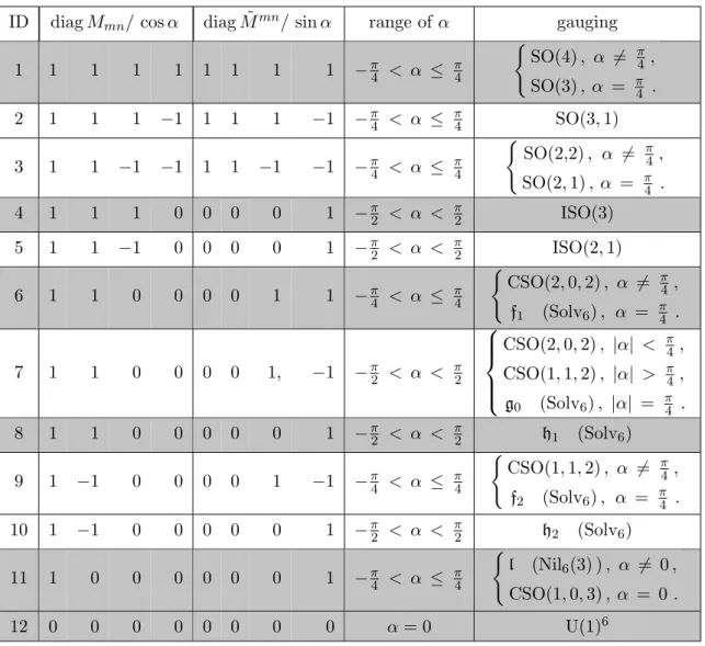
ID diagMmn/ cosα diag ˜Mmn/ sinα range ofα gauging1 1 1 1 1 1 1 1 1 −π
4 < α ≤ π4
(
SO(4), α 6= π 4 , SO(3), α = π4 .
2 1 1 1 −1 1 1 1 −1 −π4 < α ≤ π4 SO(3,1)
3 1 1 −1 −1 1 1 −1 −1 −π4 < α ≤ π4
(
SO(2,2), α 6= π 4 , SO(2,1), α = π
4 . 4 1 1 1 0 0 0 0 1 −π2 < α < π2 ISO(3)
5 1 1 −1 0 0 0 0 1 −π
2 < α < π2 ISO(2,1)
6 1 1 0 0 0 0 1 1 −π
4 < α ≤ π4 (
CSO(2,0,2), α 6= π4,
f1 (Solv6), α = π4 .
7 1 1 0 0 0 0 1, −1 −π2 < α < π2
CSO(2,0,2), |α| < π4,
CSO(1,1,2), |α| > π 4,
g0 (Solv6), |α| = π4 . 8 1 1 0 0 0 0 0 1 −π2 < α < π2 h1 (Solv6)
9 1 −1 0 0 0 0 1 −1 −π4 < α ≤ π4
(
CSO(1,1,2), α 6= π 4,
f2 (Solv6), α = π4 . 10 1 −1 0 0 0 0 0 1 −π2 < α < π2 h2 (Solv6)
11 1 0 0 0 0 0 0 1 −π4 < α ≤ π4
(
l (Nil6(3) ), α 6= 0,
CSO(1,0,3), α = 0.
12 0 0 0 0 0 0 0 0 α = 0 U(1)6
Table 1. Solutions of the embedding tensor for half-maximal, electrically gauged supergravity in
n= 3 dimensions. All shaded entries give rise to compact groups. Details about f1, f2, g0,h1 and
h2can be found in [15]. All compact solution are also discussed in appendixAin detail.
Since the matrixMnp is symmetric, one can always find a SO(4) rotation to diagonalize it. This group is the maximal subgroup of SL(4) and is up toZ2 isomorphic to SO(3)×SO(3), the maximal compact subgroup of SO(3,3). Hence, there is always a double Lorentz transformation that can be applied to the structure coefficients to diagonalize Mnp. If Mnp is diagonal, ˜Mrq is diagonal, too. Otherwise, equation (3.12) would be violated. This observation allows us to solve the quadratic constraint. In total, one finds the eleven different non-trivial solutions [15] presented in table 1. All of them depend on one real parameter α. The shaded ones are compact2 and thus the appropriate starting point for
2Note that groups like ISO(3) or CSO(2,0,2) are of course in general not compact. However, one is able
to make them compact by identifying various points. In the same way a compactD-tours arises from the non-compact planeRD. As discussed e.g. in [25], this procedure puts restrictions on the background fluxes
JHEP02(2016)039
a compactification. For completeness, we also added the trivial solution 12 with vanishingstructure coefficients. It arises after a compactification on a T3. Note that only the solutions 1,2 and 3 give rise to semisimple Lie groups. The others correspond to solvable and nilpotent Lie groups. Appendix A shows how to construct the DFTWZW background generalized vielbein EAI for all shaded, compact solutions.
3.2 Original DFT
In this subsection, we review generalized Scherk-Schwarz compactifications in the original flux formulation. In order to perform a compactification, it is essential to distinguish between internal, compact and external, extended directions. In the following we assume that there are n internal and D−n external ones. To make this situation manifest, we split the flat and curved doubled indices used in original DFT into the components
VA¯=Va Va VA
and WI¯=Wµ Wµ WI
. (3.13)
Lowercase indices like aand µdescribe external directions and thus run from 0 to D−1, while A and I parameterized the internal, 2n-dimensional doubled space. In this conven-tion, the O(D, D) invariant metric reads
ηM¯N¯ =
0 δνµ 0 δν
µ 0 0 0 0 ηM N
, η
¯ MN¯ =
0 δν µ 0 δνµ 0 0 0 0 ηM N
(3.14)
and the flat generalized metric is defined as
SA¯B¯ =
ηab 0 0 0 ηab 0 0 0 SAB
, S
¯ AB¯ =
ηab 0 0 0 ηab 0 0 0 SAB
. (3.15)
The curved version of the generalized metric arises after applying the twisted generalized vielbein [9,11,12]
EA¯M¯(X) =EbA¯N¯(X)UNˆMˆ(Y) with U ˆ N ˆ M =
δνµ 0 0 0 δν
µ 0 0 0 UNM
(3.16)
to the flat version SA¯B¯, resulting in
HM¯N¯ =E ¯ A ¯ MSA¯B¯E
¯ B ¯
N. (3.17)
This twisted vielbein implements a special case of the generalized Kaluza-Klein ansatz [13] called generalized Scherk-Schwarz ansatz. It is a product of two parts: while the generalized vielbein
b
EA¯M¯ =
eαµ −eαρCµρ −eαρAbM ρ 0 eα
µ 0
0 EbA
LAbLµ EbAM
with Cµν =Bµν+ 1 2Ab
L
JHEP02(2016)039
which combines all dynamic fields of the effective theory, only depends on the externalcoordinates X, the twistUNM just depends on the internal coordinates Y. All quantities it has a non-trivial action on are induced by a hat. For simplicity, we assume that the generalized dilaton dis constant in the internal space. Moreover, the twist further has to fulfill the following constraints [9,12,15,22]:
• Only O(n, n)-valued twists with the defining property
UIKηKLUJL=ηIJ (3.19)
are allowed.
• The structure coefficients of the effective theory’s gauge algebra
FIJ K = 3U[IL∂LUJMUK]M = const. (3.20)
have to be constant.
• The structure coefficients have to fulfill the Jacobi identity
FM[IJFMK]L= 0. (3.21)
Note that these properties imply that the structure coefficients FIJ K are solutions of the embedding tensor, which we discussed in the last subsection.
Using them, one is able to calculate all components of the covariant fluxes
FA¯B¯C¯ = 3E[ ¯AI∂IEB¯JEC]J¯ and (3.22)
FA¯=EBI¯ ∂IEB¯JEAJ¯ + 2EA¯I∂Id with d=φ− 1
2log dete a
µ. (3.23)
Remember that these two definitions differ significantly from the ones used in DFTWZW. After some algebra, one obtains the non-vanishing flux components [9,13]
Fabc=eaµebνecρGbµνρ Fabc = 2e[aµ∂µeb]νecν =fabc FabC =−eaµebνEbCMFbMµν FaBC =eaµDbµEbBMEbCM
FABC = 3Ω[ABC] Fa=fabb + 2eaµ∂µφ . (3.24)
These equations are written in a manifest gauge covariant way, by using the gauge covariant derivative
b
DµEbAM =∂µEbAM − FMJ IAbJµEbAI. (3.25)
The corresponding field strength
b
FMµν = 2∂[µAbMν]− FMN LAbNµAbLν (3.26)
is defined as usual in Yang-Mills theories. It fulfills the Bianchi identity
JHEP02(2016)039
Furthermore, the canonical field strength for the B-field, Bij, is extended by aChern-Simons term in order to be invariant under gauge transformations. The resulting 3-form
b
Gµνρ= 3∂[µBνρ]+ 3∂[µAbMνAbM ρ]− FM N LAbMµAbNνAbLρ (3.28)
also fulfills a Bianchi identity, namely
∂[µGνρλ]= 0. (3.29)
Plugging the covariant flux (3.24) into the action of the original flux formulation
S= Z
d2DX e−2d
FAFBSAB+ 1
4FACDFB
CDSAB
− 121 FABCFDEFSADSBESCF
−16FABCFABC− FAFA
(3.30)
and switching to curved indices, we finally arrive at the effective action [9,13]
Seff = Z
dD−nx√−g e−2φ
R+ 4∂µφ ∂µφ− 1
12GbµνρGb µνρ
− 14HbM NFbM µνFbNµν+ 1
8DbµHbM NDb µb
HM N−V
, (3.31)
with the scalar potential
V =−1 4FI
KLF
J KLHbIJ + 1
12FIKMFJ LNHb IJ b
HKLHbM N +1 6FIJ KF
IJ K. (3.32)
Here,Rdenotes the standard scalar curvature in the external directions. As a consequence of the generalized Scherk-Schwarz ansatz, the Lagrange density of DFT is constant in the internal directions. Thus, it is trivial to solve the action’s integral in these directions. The resulting global factor is neglected. As expected, the action (3.31) describes a bosonic subsector of a half-maximal, electrically gauged supergravity. It is equivalent to the one presented by [22].
JHEP02(2016)039
3.3 DFT on group manifolds
Equipped with the flux formulation of DFTWZW, we now perform a generalized Scherk-Schwarz compactification and present the resulting low energy effective action. Throughout the following calculations, we have to distinguish between n compact, internal directions and D−n extended, external directions, corresponding to the internal coordinates Y and external coordinates X, respectively. To make this situation manifest, we split the three different types of indices, which are relevant for the flux formulation derived in the last sections, according to
VAˆ˜=Vˆa Vˆa VAˆ
WB˜ =Wb Wb WB
XM˜ =Xµ Xµ XM
. (3.33)
This step is equivalent to the strategy in DFT. There is only the difference that we have to treat three different kinds of indices (hatted, flat and curved) with this splitting, while DFT has only two, as it does not possess a background vielbein. The external indices ˆa,a
andµrun from 0 to D−n−1 and their internal counterparts ˆA,AandM parameterize a 2n-dimensional, doubled space. This index convention gives rise to three different versions of the η-metric
ηAˆ˜Bˆ˜ =
0 δaˆ ˆb 0 δˆaˆb 0 0 0 0 ηAˆBˆ
ηA˜B˜ =
0 δa b 0 δab 0 0 0 0 ηAB
ηM˜N˜ =
0 δµ ν 0 δµν 0 0 0 0 ηM N
(3.34)
that are used to lower the indices defined in (3.33). Moreover, we use the flat, background generalized metric
SAˆ˜Bˆ˜ =
ηaˆˆb 0 0 0 ηaˆˆb 0 0 0 SAˆBˆ
and its inverse S ˆ ˜ ABˆ˜ =
ηˆaˆb 0 0 0 ηaˆˆb 0 0 0 SAˆBˆ
. (3.35)
For the next step, we specify the Scherk-Schwarz ansatz of the composite generalized viel-bein
EAˆ˜M˜ = ˜EAˆ˜B˜(X)EB˜M˜(Y). (3.36) Its fluctuation part only depends on the external coordinatesX, while the background part only depends on the internal ones Y. In comparison with the ansatz in [9,12,13,22], the background generalized vielbein EB˜
˜
M takes the role of the twist UNˆ ˆ
M. As opposed to the twist, it is not restricted to be O(D, D) valued. This observation solves the problem of constructing an appropriate twist: there is always a straightforward way to construct
EB˜ ˜
M as the left-invariant Maurer Cartan form on a group manifold. We went through this process for the example ofS3 withH-flux in [25].
For the fluctuation vielbein ˜EAˆ˜B˜, the generalized Kaluza-Klein ansatz [9, 12, 13] is adapted to the index structure introduced above and gives rise to
˜
EAˆ˜ ˜ B(
X) =
ebˆa 0 0 −eˆacCbc eˆab −eˆacAbBc b
EAˆCAbCb 0 EbAˆB
with Cab =Bab+ 1 2Ab
D
JHEP02(2016)039
In this ansatz, Bab denotes the two-form field appearing in the effective theory andb
HCD =EbAˆCSAˆBˆEbBˆD (3.38)
representsn2 independent scalar fields which form the moduli of the internal space. Anal-ogous to the twist, the background vielbein has only non-trivial components in the internal space and reads
EB˜M˜(Y) =
δb
µ 0 0 0 δbµ 0 0 0 EBM
. (3.39)
With the Kaluza-Klein ansatz (3.37) and the partial derivative
∂M˜ =∂µ ∂µ ∂M
(3.40)
in mind, it is straightforward to calculate the fluxes ˜FAˆ˜Bˆ˜C˜ˆ and ˜FAˆ˜ defined in (2.33) and (2.36). After some algebra, we obtain the non-vanishing components
˜
Fˆaˆbˆc =eaˆdeˆbeecˆf3 D[dBef]+AbD[dDeAbDf]
˜
Fˆaˆbˆc = 2e[ˆadDdeˆb]eeecˆ= ˜faˆˆcˆb ˜
FˆaˆbCˆ =−eˆadeˆbeEbCDˆ 2D[dAbDe] F˜ˆaBˆCˆ =eˆa dD
dEbBˆ DEb
ˆ CD ˜
Fˆa= ˜fˆaˆˆcc+ 2eˆabDbφ . (3.41)
In order to determine the covariant fluxes FAˆ˜Bˆ˜Cˆ˜, we also have to evaluate the background contribution FAˆ˜Bˆ˜Cˆ˜. As the background vielbein (3.39) only depends on internal coordi-nates, the only non-vanishing components ofFA˜B˜C˜ are
FABC = 2Ω[AB]C. (3.42)
They give rise to the non-vanishing components
Fˆaˆbˆc =−eaˆdeˆbeecˆfAbdDAbeEAbfFFDEF FaˆˆbCˆ =eˆadeˆbeAbcDAbdEEbCˆ FF
DEF FˆaBˆCˆ =−eaˆ
bAb bDEbBˆ
EEb ˆ C
FF
DEF FAˆBˆCˆ =EAˆ DE
ˆ B
EE ˆ C
FF
DEF. (3.43)
Combining these results with (3.41) and remembering the gauge covariant quantities
b
DµEbAˆ B=∂
µEbAˆ B
−FBCDAbµCEbAˆ D b
FAµν = 2∂[µAbν]A−FABCAbµBAbνC b
Gµνρ= 3∂[µBνρ]+Ab[µA∂νAbρ]A−FABCAbµAAbνBAbρC, (3.44)
discussed in section 3.2, we finally obtain
Fˆaˆbˆc =eˆa µe
ˆ b
νe ˆ
cρGbµνρ Fˆaˆbˆc = 2e[ˆaµ∂µeˆb]νeνˆc FaˆˆbCˆ =−eaˆ
µe
ˆbνEbCAˆ FbAµν FaˆBˆCˆ =eaˆµDbµEbBˆAEbCAˆ FAˆBˆCˆ =EbAˆ
DEb ˆ B
EEb ˆ C
F F
JHEP02(2016)039
Note that the gauge covariant objects here carry indicesA, B, C,· · · instead ofI, J, K,· · ·,as they do in the last subsection. This is because they have to carry O(n, n) indices, which are the former for DFTWZW(depicted in (2.26)) and the latter in the original formulation. From this point on, all further calculations proceed as explained in the last subsection. Thus, when substituting our results into the flux formulation’s action of DFTWZW (2.55), we again obtain the effective action (1.8). As explained above, this time the indices
I, J, K,· · · are substituted by A, B, C,· · ·. However, this difference is mere convention. Furthermore, the scalar potential
V =−1 4FA
CDF
BCDHbAB+ 1
2FACEFBDFHb ABb
HCDHbEF (3.46)
lacks the strong constraint violating term 1/6FABCFABC, which appears as a cosmological constant in gauged supergravities, even if we do not impose the strong constraint on the background field. In section2.3.1, we argued why this term is missing in our formulation. Anyhow, from a bottom up perspective it is totally legitimate to add it by hand to the action in the same way as it was done in the original flux formulation. It is perfectly compatible with all the symmetries of the theory.
Our new approach solves an ambiguity of generalized Scherk-Schwarz compactifica-tions: in the DFTWZW framework, the twist is equivalent to the background generalized vielbein EAI. It is constructed in the same way as for conventional Scherk-Schwarz com-pactifications. This is possible, because the theory possesses standard 2D-diffeomorphisms. Thus, all mathematical tools available for group manifolds are applicable. We immediately lose these tools, if we return to the original DFT formulation, because the extended strong constraint, necessary for this transition, breaks 2D-diffeomorphism invariance. Hence, one is left with the problems outlined in subsection 3.2.
All derivations performed so far in DFTWZWare top down. It started from full bosonic CSFT in [7, 8] and was reduced step by step until we finally arrived at the low energy effective action (1.8). Thus, one is able to explicitly check the uplift of solutions of its equations of motion to full string theory. In doing so, we have to keep in mind that all results obtained so far are only valid at tree level. Consistency at loop level, e.g. a modular invariant partition function, gives rise to additional restrictions. There is another lesson which can be learned from the CFT side: we know that the background fluxesFABC scale with 1/√k, where k denotes the level of the Kaˇc-Moody algebra on the world sheet. To make this property manifest, we decompose them into
FABC = 1 √
kfABC (3.47)
and assume that the structure coefficientsfABC are normalized, e.g.
fACDfBDC = 1
2δAB. (3.48)
Now, the gauge covariant derivative reads
b
DµVA=∂µVA− 1 √
kf A
JHEP02(2016)039
From this equation, we immediately read off the Yang-Mills coupling constantgYM= 1 √
k. (3.50)
Remember, the geometric interpretation of DFTWZW only holds in the large level limit k ≫ 1. The corresponding effective theory is weakly coupled and thus can be treated perturbatively. However, freezing out all fluctuations in the internal directions, which is exactly the case for generalized Scherk-Schwarz compactifications, our results extend to
k= 1. In this case, one has to reduce the number of external directions to cancel the total central charges of the bosons and the ghost system.
3.4 Constructing the twist
A major advantage of generalized Scherk-Schwarz compactifications in DFTWZW is the existence of a straightforward procedure to construct the background vielbeinEAI, which replaces the twist in the original scenario, by starting from a solution of the embedding tensor. In the following, we present this scheme in detail.
Let us first assume that tAdenotes 2ndifferentN×N matrices which give rise to the algebra
[tA, tB] =tAtB−tBtC =FABCtC. (3.51)
Its structure coefficients are equivalent to an arbitrary solution of the embedding ten-sor (3.1). In this case
FABDηDC+FACDηBD= 0 (3.52)
has to hold. Furthermore, we define a non-degenerate, bilinear, symmetric two-form
K(tA, tB) =ηAB (3.53)
on the vector space spanned by the matricestA. Later, we will explain how they and the two-form are realized. At the moment, these three definitions are sufficient. With them, it is evident that the background fluxes FABC are given by
FABC =K(tA,[tB, tC]). (3.54)
The second ingredient, required to derive the background generalized vielbein, is a group element g ∈G of the groupG representing the background. Therefore, we use the exponential map
g= exp(tAXA) =
∞
X
m=0 1
m!(tAX
A)n (3.55)
in order to derive it from the generatorstA. For compact groups this map is surjective onto the identity componentG0 ofG. We assume that all groups we treat here are path-connect and thus G0 and G are equivalent. The map (3.55) becomes bijective, if we restrict the domain of the coordinatesXI accordingly. In this case, each group element is labeled by a unique point in the coordinate space. The left invariant Maurer-Cartan form is defined as
JHEP02(2016)039
Using it to calculateΩABC =EAI∂IEBJECJ, (3.57)
we obtain
ΩABC =−EAIK(tC, ∂Ig−1gg−1∂Jg) +K(tC, g−1∂I∂Jg)EBJ =EBJK(g−1∂Jg, tCg−1∂Ig)EAI − K(tC, g−1∂I∂Jg)EAIEBJ
=K(tB, tCtA)− K(tC, g−1∂I∂Jg)EAIEBJ. (3.58)
The coefficients of anholonomy give rise to the correct background covariant fluxes, namely
FABC = 2Ω[AB]C =K(tA,[tB, tC]). (3.59)
Thus, we indeed recover the correct identity for the background generalized vielbein EAI, with the left invariant Maurer-Cartan form (3.56).
As already stated, the generators tAof the Lie algebra are N ×N matrices
tA=
(tA)11 · · · (tA)1N ..
. ...
(tA)N1 · · · (tA)N N
. (3.60)
In order to evaluate K(x, y) for arbitrary algebra elements x, y ∈ g, we need to expand them in terms of the generators, e.g.
x= 2n X
A=1
cAtA, (3.61)
wherecA denotes the 2nexpansion coefficients. It is convenient to rearrange the matrix x into the vector
x=x11 · · · x1N x2N · · · xN N
(3.62)
and solve the linear system of equations
cM =x with M =
(t1)11 · · · (t1)1N (t1)2N · · · (t1)N N ..
. ... ... ...
(t2n)11 · · · (t2n)1N (t2n)2N · · · (t2n)N N
and c=
c1 · · ·c2n
(3.63) to calculate these coefficients. We are interested in a unique solution, thus the 2n×N2
matrixM has to have full rank
rankM = 2n . (3.64)
JHEP02(2016)039
3.4.1 Semisimple algebras
For semisimple Lie algebras, the generators
(tA)BC =FABC (3.65)
can be read off directly from the structure coefficients. Doing so, we obtain the adjoint representation
adxy= [x, y] with x, y ∈g (3.66) in the basis spanned by all abstract generators. It has dimensionN = 2nand is faithful if the center of the Lie algebra
Z(g) ={x∈g|[x, y] = 0 for all y∈g} (3.67)
is trivial. This is the case for semisimple Lie algebras. However, there are also non-semisimple ones, such as ISO(3) which is discussed in appendixA.2, with vanishing center. The matrix realization of their generators is given by (3.65), too.
In general, the adjoint representation is not the lowest dimensional one. E.g. for SO(4), which we present in appendix A.1, the adjoint has N = 6, while the fundamental representation is only 4-dimensional. In the end, each of them works for our purpose. However, taking the smallest one simplifies the calculations considerably.
3.4.2 Nilpotent Lie algebras
For nilpotent Lie algebras, (3.65) gives rise to generatorstA which are not linear indepen-dent from each other. Thus, they are not faithful and violate (3.64). Before discussing how to obtain proper generators, let us first give a criterion to identify these algebras. To this end, consider the lower central series
Lm+1 = [g, Lm] with L0=g. (3.68)
It gives rise to the series
g=L0 ⊇L1 ⊇L2 ⊇. . . (3.69)
of subalgebras. If this series terminates at a finite k with Lk = {0}, the algebra g is nilpotent of orderk.
In the following we make use of the infinite dimensional universal enveloping algebra U(g) of the nilpotent Lie algebrag. According to the Poincar´e-Birkhoff-Witt theorem, it is spanned by the ordered monomials
t(α) =tα1
1 tα22. . . tα2 n
2n with α∈Z3+. (3.70)
Via left multiplication
φx : U(g)→U(g), φx(y) =xy with x∈g, (3.71)
algebra elements x act faithful on the universal enveloping algebra. Ado’s theorem states that even on the finite dimensional subspace