VARIABILITY IN THE COLORED AND FLUORESCENT DISSOLVED ORGANIC MATTER WITH SALINITY IN THE NEUSE RIVER ESTUARY
George T. Dang
A thesis submitted to the faculty of the University of North Carolina at Chapel Hill in partial fulfillment of the requirements for the degree of Master of Science in the Department of Environmental Sciences and Engineering.
Chapel Hill 2011
Approved by:
Dr. Rose M. Cory
Dr. Hans W. Paerl
ABSTRACT
GEORGE T. DANG: Variability in the Colored and Fluorescent Dissolved Organic Matter with Salinity in the Neuse River Estuary
(Under the direction of Dr. Rose M. Cory)
The chromophoric and fluorescent dissolved organic matter (CDOM and FDOM,
respectively) were examined in the Neuse River Estuary (NRE), North Carolina, USA, to
assess the spatial and temporal variation in dissolved organic matter (DOM) quantity and
quality. Trends of quantity and quality measurements were coupled to seasonal discharge
and hydrologic mixing regimes. Differences between spectral measurements of DOM
between low and high salinity datasets revealed differences in the CDOM and FDOM
behavior along salinity gradients. Variability in the fluorescence character of DOM between
the low and high salinity datasets revealed difficulties using fluorescence as a tracer for
DOM along the salinity gradient in the NRE. Although fluorescing components with similar spectra were identified, differences in the fluorescing DOM components constrained a
whole-system analysis of FDOM. While this study improved dissolved organic matter
characterization of the NRE, it also revealed challenges with utilizing fluorescent properties
iii
AKNOWLEDGEMENTS
I would like to formally thank my advisor Dr. Rose Cory for mentoring me and for all
the hard work she dedicated to making this project and thesis a reality. I would also like to
thank Dr. Hans Paerl, the MODMON project, and Paerl lab group, with particular gratitude
to Karen Rossignol, Lois Kelly, and Melissa Leonard, for the coordination, sampling, and
processing of samples for this project. Additionally I would like to think my committee
member Dr. Steve Whalen for the time and effort put into reviewing this paper. I must also
thank Dr. Jack Weiss for his aid in statistical analysis. I would finally like to thank my lab
members, Katie Harrold, Angela Wang, Collin Ward, and Rory Polera, for their support and
TABLE OF CONTENTS
LIST OF TABLES ... vi
LIST OF FIGURES ... vii
Chapter I. INTRODUCTION ...1
II. METHODS...7
Site Description ...7
Field Sampling and Sample Processing ...8
DOC Measurements ...9
Optical Measurements ...9
Parallel Factor Analysis (PARAFAC) ...12
Statistical Analysis ...14
III. RESULTS ...15
Spatial and temporal patterns in temperature, salinity, and turbidity ...15
DOC, CDOM and FDOM variability along transect ...15
PARAFAC modeling and validation ...21
IV. DISCUSSION ...24
Spatial and temporal patterns ...24
v
Impact of salinity on FDOM: EEM peak picking ...30
Effect of salinity on FDOM: PARAFAC ...32
V. CONCLUSION ...39
VI. TABLES AND FIGURES ...41
APPENDIX ...54
LIST OF TABLES
Table
3.1 Summary of descriptive statistics for physical and DOM measurements... 42
3.2 Slope and R2 of regressions of CDOM and FDOM measures vs. salinity ...47
3.3 Fluorescence characteristics of Neuse River Estuary derived
from two PARAFAC models split by salinity ...52
3.4 Regression slopes and R2 for component validation method
of comparing output loadings of two PARAFAC models ...53
A.1 Station locations and distances from upstream end-member ...54
A.2 Tukey Honest Significant Differences Test for DOM measurements
grouped by Station ...57
A.3 Tukey Honest Significant Differences Test for DOM measurements
grouped by Season ...57
A.4 Spearman rank correlation coefficients between DOM measurements
and physical explanatory variables ...68
A.5 Spearman rank correlation coefficients (ρ) and corresponding
vii
LIST OF FIGURES
Figure
2.1 Map of 11 sampling stations along the NRE ... 41
3.1 Median and interquartile ranges by station: Temperature, Salinity,
Turbidity. ... 43
3.2 Median and interquartile ranges by station: Absorbance coefficient,
DOC, SUVA254, Fluorescence index, Slope Ratio ...44
3.3 Absorbance coefficient and Slope ratio plotted against salinity ...45
3.4 Fluorescent emission peaks A, C, and T plotted against salinity...46
3.5 Percent change of Absorbance coefficient, and Fluorescent emission
peaks A, C, and T plotted against change in Salinity ...49
3.6 Fluorescence signatures and validation of the components from
PARAFAC models...50
A.1 Plot of average daily discharge of the Neuse River and air
temperature in Beaufort Country, NC over sampling period ...54
A.2 Boxplots of physical and DOM quantity and quality measurements,
grouped by season ...56
A.3 Surface and bottom DOM measurements on a representative date
with a highly stratified water column ...58
A.4 Surface and bottom DOM measurements on a representative date
with a well mixed water column ...59
A.5 Surface and bottom DOM measurements on a representative date
with a partially mixed water column ...60
A.6 Scatterplots of DOC versus Salinity and Turbidity grouped by
Station ...61
A.7 Scatterplots of Absorbance Coefficient versus Salinity,
Temperature, and Turbidity grouped by Station ...63
A.9 Scatterplots of SR versus Salinity, Temperature, and
Turbidity grouped by Station ...66
A.10 Scatterplots of SUVA254 versus Salinity and Temperature,
I. INTRODUCTION
The NRE is the largest tributary of the Pamlico Sound (PS) system of the North
Carolina outer banks. The PS is the second largest estuary and largest logoonal system in the
United States. The characteristic barrier islands of the Outer Banks shield the estuary from
the open ocean, limiting exchange to three narrow inlets. The unique geomorphology of the
sound results in long water residence times (on average of one year) and efficient use of
nutrients. The long residence times also make the system highly sensitive to nutrient
over-enrichment and eutrophication (Copeland and Gray 1991, Paerl et al. 2001, 2006). As the
largest tributary to the PS, the NRE is of particular concern due to its contribution of nutrient
loading to the system. An increase in urban areas and a substantial boom in the hog farming
industry in the Neuse River watershed over the past few decades (Stow et al. 2001), have
both likely played a role in the over-enrichment of the system.
Given that the NRE is draining an increasingly urbanizing, agricultural, and industrial
watershed, the NRE has begun to show signs of eutrophication during most years, such as
algae blooms, fish kills, and oxygen depletion (Copeland and Gray 1991, Paerl et al. 1998).
Thus, North Carolina Department of Natural Resources have classified the NRE as an
impaired system and have since then sought means to monitor and remediate the system.
While nutrient over-enrichment is the cause of harmful algal blooms and fish kills, there are
biogeochemical controls that enhance or constrain the utilization of nutrients that supports
It has long been recognized that the cycling of dissolved organic matter (DOM) is
critical for water quality, given that DOM plays numerous roles in controlling the fate of
added nutrients. For example, chromophoric DOM (CDOM) acts as a sunscreen for aquatic
ecosystems, absorbing visible and harmful ultraviolet radiation (Vahatalo et al. 2000).
CDOM thus controls the depth of the photic zone in most natural waters, including the NRE
(Vahatalo et al. 2005) and is therefore a critical control on algal productivity. Labile
fractions of DOM fuel the food web in aquatic ecosystems (Carpenter et al. 2005), and thus
the extent to which bacteria respire DOM to CO2 influences the level of dissolved oxygen in
the water. In addition, studies have suggested that certain harmful algal bloom species can
use organic compounds within the DOM pool to meet their nitrogen, phosphorous, and/or
carbon requirements—thereby influencing algal community structure (Heisler et al. 2008).
The capacity of DOM to attenuate sunlight or to facilitate the growth of aquatic
microorganisms depends on its concentration and chemical composition, which in turn
depend on inputs from allochthonous or autochthonous precursor materials. Allochthonous
sources of DOM include degrading plant and soil material delivered from the watershed
while autochthonous sources are derived from the breakdown of bacterial and algal matter in
the water column (Thurman 1985; McKnight et al. 2003). Allochthonous precursor organic
matter is enriched in light-absorbing aromatic carbon structures and low in nitrogen
(McKnight et al. 1997; McKnight et al. 2003). In contrast, autochthonous material is
relatively rich in organic nitrogen and aliphatic carbon (McKnight et al. 1997; McKnight et
al. 2003). Thus, on a per carbon basis, terrestrially-derived DOM delivered from the
3
the absorption of specific wavelengths of the light utilized by a subset of species (Vahatalo et
al. 2005).
While the importance of DOM on water quality is widely recognized, challenges
remain in understanding how DOM’s roles in water quality depend on its source and
chemical composition. The quantity, source and chemical composition of aquatic DOM in
streams is dynamic, exhibiting short-term fluctuation on diurnal scales from
photodegradation (Spencer et al. 2007, Cory et al. 2007) or from storm event driven inputs of
DOM (Carstea et al. 2009, Fellman et al. 2009). Seasonal variability in aquatic DOM
quality arises due to changing biogeochemical processes in the watershed. Examples of these
processes include: input of leaf litter during senescence (McDowell and Fisher 1976) and
long term patterns of change in response to shifts in climate, land use, or other perturbations
in the watershed (Monteith et al. 2007, Wilson and Xenopoulos 2008).
Because DOM quantity and composition reflect a dynamic interplay between organic
matter sources and biogeochemical processes (Jaffé et al. 2008), land use and urbanization
are expected to have an effect on the shift in the concentration and chemical signatures of
DOM, which will in turn control the response of aquatic systems to nutrient enrichment.
Thus, understanding the dynamic roles of DOM in aquatic systems requires measures of
DOM quality on the timescale of hours to days (Kaplan et al. 2008), a temporal resolution
that may be achieved by the increasingly rapid optical analyses of the chromophoric
(CDOM) and fluorescent (FDOM) fractions of the DOM pool, which serve as proxies for
DOM quantity, source, and chemical composition. For example, specific UV absorbance at
254 nm (SUVA254) by CDOM is strongly correlated to the aromatic carbon content of the
al. 1997). Similarly, analysis of FDOM signals observed in an excitation emission matrix
(EEM) via parallel factor analysis (PARAFAC) is increasingly used to assess DOM
dynamics in aquatic systems (Stedmon et al. 2003). This approach provides insight into
different types of carbon within the DOM pool hypothesized to represent classes of carbon
varying in lability to bacteria: carbon associated with humic substances derived from either
terrigenous or microbial sources, and carbon associated with free or combined fluorescent
amino acids, specifically tryptophan, tyrosine, and phenylalanine.
Evaluating changes in CDOM and FDOM along riverine to estuarine transects is
increasingly proposed as a way to understand the linkages between DOM source and its roles
in water quality. For example, the extent to which terrestrial DOM is broken down into other
forms while traveling downstream, reflected in loss in DOM concentration and shifts in
CDOM and FDOM signals, provides information on the biogeochemical processes
controlling DOM degradation (Kowalczuk et al. 2009, Astoreca et al. 2009, Singh et al.
2010). However, there are several challenges to this approach. First, freshwater is constantly
being diluted as it is entering the estuary because freshwater is coming into contact with
low-DOM seawater in addition to tributary inflow containing different quantity and quality of
DOM. The mixing of freshwater and seawater also introduces marine sources of DOM to the
system (de Souza Sierra et al. 1997), which are degraded humic material and microbial
production byproducts (Nguyen et al. 2005, Suksomjit et al. 2009). For these reasons, it is
difficult to attribute reduction in DOM concentration and shifts in DOM quality to the
breakdown of terrestrial DOM vs. conservative mixing of terrestrial DOM with marine DOM.
5
The task of decoupling the effects of DOM processing and mixing is complicated by
the variations in hydrodynamic patterns in estuaries. Influenced by factors such as upstream
discharge, wind velocity and direction, and internal seiching, the NRE can experience
significant variations in flow pattern and stratification on the scale of hours to days (Luettich
et al. 2001, Luettich 2002). If DOM dynamics are highly influenced by mixing from the
freshwater and marine end-members, it may be difficult to distinguish actual trends from
variable noise without frequent sampling or long term monitoring coupled to studies of the
hydrodynamics.
Lastly, one additional challenge to using CDOM and FDOM as tracers for DOM
dynamics along riverine to estuarine transects is that the changes in salinity that occur along
these gradients can alter CDOM and FDOM signals (Mobed et al. 1996, Boyd 2004,
Batchelli et al. 2009, Stephens and Minor 2010, Boyd et al. 2010). Arguably, the effect of
salinity on FDOM signals is expected to be greater than effects on CDOM signals because
emission of fluorescence is highly dependent on the local chemical environment surrounding
the fluorescing moiety. Thus, studies have attempted to determine the specific effects of
salinity on FDOM signals, and they have so far determined that effects of salinity may be
important but are not constant across all systems.
Studies have suggested that the fluorescent signatures of certain types of FDOM may
exhibit shifts in peak positions and change in fluorescence intensity along a salinity gradient.
Lakowicz (1999) demonstrated that shifting of amino acid-like fluorescence towards shorter
wavelengths (blue-shifting) occurs when there is a decrease in solvent polarity, and shifts to
longer wavelengths (red-shifting) occurs within solutions with increased solvent polarity.
along a salinity gradient where water becomes less polar as salt concentration increases.
Simulated mixing transects in a study by Boyd et al. (2010) have also suggested that
fluorescence intensities of DOM fluorophores change with respect to salinity and that FDOM
samples from different estuaries and regions within an estuary behaved differently. These
studies suggest that the impact of salinity on fluorescence is not well understood and is
variable between different natural systems. Therefore, salinity effects must be further
examined in specific systems in order to utilize FDOM as an accurate tracer for DOM in
estuarine systems.
Thus, my research goal was to test the effects of salinity on CDOM and FDOM in the
NRE. Using the natural variability in FDOM and salinity in the NRE, I employed parallel
factor analysis (PARAFAC) to resolve datasets of FDOM into their underling components as
a function of salinity, and compared patterns in these FDOM signals to composite FDOM
II. METHODS
2.1 Site Description
The Neuse River Estuary (NRE) is the largest tributary and nutrient contributor to the
Albemarle-Plamlico Estuarine System (APES), located on the central Atlantic seaboard
along the coast of North Carolina, U.S.A. (34.97660°, 76.87550°). The Neuse River
watershed runs from the Piedmont though the costal plains of North Carolina, draining an
area of 1.62 x 10⁴ km2. Despite comprising only 20% of the of total drainage area of the
APES, the Neuse contributes 35% of the N and 50% of the P loadings to the system (Spruill
1997). Land use estimates in 2001 from the USDA have indicated the watershed to be
composed of 38% forests, 29% agriculture, 14% wetlands, and an expanding 13% of urban
areas.
The NRE spans ~70 km in length. The system is both broad and shallow with an
average width and depth of ~6.5 km and ~2.7 m respectively (Luettich 2002, Paerl et al.
2010). River discharge and flushing time of he estuary can range between 50-1,000 m3s-1 and
7-200 days respectively (Paerl et al. 2010). The region experiences a four season climate
where water temperature may typically ranges between ~3.4-33.6 °C (Peierls and Paerl 2010).
Salinity of the system ranges from ~0-29.2 practical salinity units (PSU) along the
70km transect (Peierls and Paerl 2010). Exhibiting several flow regimes governed by
discharge volume, wind direction and velocity, and internal seiching, the NRE also often
the NRE exhibited: classical estuarine circulation (with surface water moving downstream
and bottom water moving upstream) 52 percent of the time; downstream riverine circulation
(both surface and bottom flow downstream) 36 percent of the time; anti-riverine circulation
(both surface and bottom movement upstream) 7 percent of the time; and reverse estuary
circulation (where surface water moves upstream and bottom water moves downstream) 5
percent of the time. Thus, depending upon the source and direction of movement of the
water, the vertical salinity profile may variably stratify. The same study has determined that
discharge, wind direction, and internal seiching are the major drivers in the NRE’s
circulation and stratification. It was additionally found that influence by tides on the system
was marginal due to the laggonal nature of the downstream Pamlico Sound, which is
bounded by the Outer Banks that separates the system from the open ocean (Paerl and Peierls
2008). The study determined that winds oriented towards the southwest (up the estuary)
tended to mix the water column; where as winds oriented towards the northeast (down the
estuary) increased surface freshwater flow and enhanced stratification.
2.2 Field Sampling and Sample Processing
Samples were collected as part of the MODMON (www.unc.edu/ims/neuse/
modmon/) long-term water quality monitoring project. Bi-weekly (during the spring through
fall) to monthly (during the winter) sampling was conducted at 11 stations along an ~73km
transect (Figure 2.1). Typically cruises spanned mid-morning to mid-afternoon and began at
the furthest downstream station (station 180) and concluded at the freshwater end-member
(station 0). At each station, both surface (~1m below surface) and bottom (~1m above floor)
9
conductivity, chlorophyll a, dissolved oxygen, and pH. In total there were 22 sampling trips
and 474 samples collected between August 2009 and October 2010.
Water samples were vacuum filtered through pre-combusted 0.7 µm nominal pore
size glass fiber filters (GF/F; Whatman, Maidstone, Kent, UK) within 24 hours of collection
at UNC-CH Institute of Marine Science in Morehead City, NC. Filtrate was stored in
pre-combusted amber glass vials. Samples were then refrigerated at ~4°C until transported on
ice to UNC-CH in Chapel Hill, NC for analysis of the absorbing and fluorescent fraction of
DOM (CDOM and FDOM, respectively).
2.3 DOC Measurements
DOC analysis was conducted by the Pearl lab at UNC-CH Institute of Marine
Sciences. DOC was measured for stations 0, 30, 70, 100, 120, and 160 following the
protocols described in Vahatalo et al. (2005).
2.4 Optical Measurements
The UV-Visible absorbance spectrum was measured using a Hewlett Packard 8452A
Diode Array Spectrophotometer (Olis instruments, Bogart, GA, U.S.A.). Absorbance was
collected between 200-700 nm at 1 nm increments. Samples were measured in 1 cm or 10
cm quartz cuvettes depending on the level of absorbance of the sample. Sample absorbance
values were made in reference to laboratory DI water.
Naperian absorbance coefficients (aλ) were calculated at 300 nm as follows:
aλ=
Aλ
Where λ is the wavelength in nanometers, A is the absorbance (unitless) and l is the path length in meters.
The absorbance spectrum of DOM shows an exponential decay with increasing
wavelength, and the slope of the exponential decay has been related to measures of DOM
source and reactivity (Vodacek et al. 1997, Stedmon et al. 2001, Helms et al. 2008). The
spectral slope ratio (SR) was calculated as the ratio of the slopes (S) of the log-transformed Naperian absorbance coefficient spectra between 275-295 nm and 350-400 nm according to
Helms et al. (2008):
The spectral slope ratio is inversely correlated to average molecular weight of the DOM pool
(Helms et al. 2008).
The specific absorbance at 254 nm (SUVA254) is a proxy for aromatic carbon
content(Weishaar et al. 2003, Cory et al. 2007). SUVA254, was calculated as the absorbance
(A; unitless) at 254 nm divided by the path length (l) and normalized to the concentration of DOC (mg C L-1):
SUVA
254=
A
254l
[
DOC
]
Excitation-emission matrices (EEMs) were collected using a Florolog-321
Spectrofluorometer (Horiba Jobin Yvon Edison, NJ, U.S.A) with a charge-coupled device
Sr =S275−295 S350−400
Eqn 2
11
the an excitation range of 240-450 nm by 5 nm increments, with the detection of emission
covering 320-550 nm. Integration times ranged from 1.0-1.75 seconds at a binning of 1, for
maximum dynamic range of each sample. The pairing of integration time depended on the
UV-Vis absorbance measurement of the sample made prior to fluorescence analysis. Best
dynamic range was selected to maximize detection of emission at low wavelength.
Only one replicate EEM per sample was analyzed for samples collected between
October 26, 2009 and April 28, 2010. Beginning April 28, 2010, triplicate EEMs were
analyzed on each sample to determine instrumental error for the analysis of fluorescent DOM
(FDOM).
EEMs were corrected for inner-filter effects and instrument-specific excitation and
emission corrections using MATLAB (v7.8) following the method in Cory et al. (2010). A
User-generated rhodamine spectrum was used for excitation corrections (DeRose et al. 2009)
and a manufacturer provided emission correction spectrum (Horiba Scientific) was used for
emissions corrections. Multiple blank EEMs with laboratory DI water for each integration
time were measured daily, and were subtracted from sample EEMs to minimize the influence
of water Raman peaks. Intensities of the EEM were then converted to Raman units using the
Raman area of the associated bank (Stedmon et al. 2003).
The corrected EEM’s fluorescence index (FI, (McKnight et al. 2001), which is a relative measure of DOM source, was calculated by the ratio of emission intensity (I) at 470 nm to 520 nm at an excitation wavelength of 370 nm (Cory et al. 2010).
High values of FI imply the DOM is more derived from microbial sources while lower values
of DOM imply more terrestrial sources.
FI =I370,470
2.5 Parallel Factor Analysis (PARAFAC)
The PARAFAC approach decomposes a data set of EEM into fluorescence signals of
mathematically and chemically independent components multiplied by their excitation and
emission spectra. The process takes three-dimensional data (EEM) and decomposes into
two-dimensional data (a component’s excitation-emission spectra). Each component may
represent a single fluorophore but likely represents a group of similar and/or groups of
co-varying fluorophores (Stedmon et al. 2003, Stedmon and Bro 2008).
The PARAFAC’s algorithm utilizes an alternating least squares algorithm that
minimizes the sum of least squared residuals of an array of EEMs. The EEM dataset is
decomposed into sets of tri-linear terms and a residual array:
xi jk= ai fbj fck f +ei jk
f=1
F
∑
Where xijk is the fluorescence intensity of sample i measured at an emissions wavelength of j and an excitation wavelength of k, of a model with F components. The variables a, b, and c respectively represent the estimated relative concentration, emission spectra, and excitation
spectra of a fluorophore by the model. And the e term accounts for the unexplained noise and un-modeled variation.
PARAFAC was run and validated using the DOMFluor Toolbox in Matlab (v7.8)
following Stedmon and Bro (2008). Once outliers were removed from the dataset, models
were validated using four-way split-half analysis in which emissions and excitation spectra
13
PARAFAC modeling outputs relative concentrations of components within each
sample. It is not possible to relate PARAFAC output to actual concentrations of FDOM
components because in a complex mixture, we do not know the relationship between the
molar absorptivity, fluorescence quantum yield, and the identity and concentration of any
given FDOM component. Instead, a relative scale derived from the fluorescence intensity
called “Fmax” is used. Fmax is calculated from the fluorescence intensity of each component at its excitation and emission maxima, is measured in Raman units (RU), and is proportional to
the product of the molar absorptivity and fluorescence quantum yield of the component
(variables b an c in Eqn 5 above). Thus, Fmax values provide a way to investigate relative differences in FDOM components between samples (Stedmon and Bro 2008).
PARAFAC model fit was evaluated by comparing the residuals between the
measured EEM and modeled EEM. Residuals were output as an EEM contour plot
calculated by the fluorescence intensity in the measured EEM minus the fluorescence
intensity of the modeled EEM. Peaks in residual EEMs indicate variability in FDOM not
captured by the PARAFAC model Conversely, valleys of negative fluorescence in residual
EEMs indicate where the model over-fit emission intensity. A good fit that accurately
describes the variable in the dataset minimizes residual peaks and valleys.
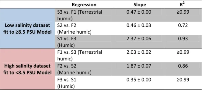
The Tucker congruence coefficient (TCC; Tucker 1951) was utilized to quantify the
similarity among components validated in the two different models (< 8.5 and ≥ 8.5 PSU
models). The congruence test calculates a standardized measure of proportionality of
elements in two vectors (excitation and emission loadings). The equation for the coefficient
Where x and y are loadings of variable i on factor x and y with i=1,..,n. For coefficient values greater than 0.92, components are considered to have a ‘good’ degree of similarity, and for
values greater than 0.98, components can be considered equivalent (Lorenzo-Seva and Berge
2006, Murphy et al. 2008).
2.6 Statistical Analysis
All statistical analysis was done in R statistical software (v 1.4). Correlations were
computed using the Spearman’s rank correlation test, a non-parametric correlation test that
accounts for data that may not meet assumptions of normality, homoscedasticity, and
linearity. The non-parametric Kruskal-Wallis rank sum test was used to compute differences
for one-way grouped data between Season, Station, and Depth. Significant differences
between the means of individual stations were calculated using the Tukey HSD (Honestly
Significant Difference) test. Simple linear regressions grouped by stations were computed
using the “lattice” package in R and fit with averaging smoothing splines.
θ
(x,y)=∑
xiyixi2
∑
yi2III. RESULTS
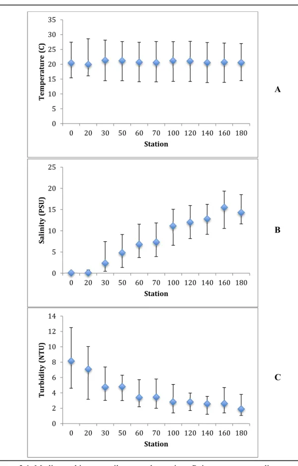
3.1 Spatial and temporal patterns in temperature, salinity, and turbidity
Over the course of the study there were no spatial trends in water temperature (Figure
3.1 A). As expected, water temperature varied consistently at all stations by season, with
greatest temperatures in the summer, cooler temperatures during the spring and fall, and
coldest temperatures during the winter (Appendix Figure 2 C). Salinity was low at stations 0
to 20, and then generally increased with distance downstream toward station 180 (Figure 3.1
B). Discharge and salinity were inversely related during the spring and winter when
discharge was high and median salinities were low (Appendix Figures 1 & 2 A, B). In the
fall and summer when discharge was low, median salinities were higher than the high
discharge winter and spring months. Turbidity was greatest at the upstream stations and
generally decreased downstream to station 180, the downstream end-member in this study.
Consistently, the variability in turbidity was greatest at the upstream stations, where the
interquartile range varied by a factor of three compared to downstream stations where ranges
varied by a factor of two (Figure 3.1 C). Turbidity was greatest during the winter and spring
seasons, reflecting discharge (Appendix Figure 2 D).
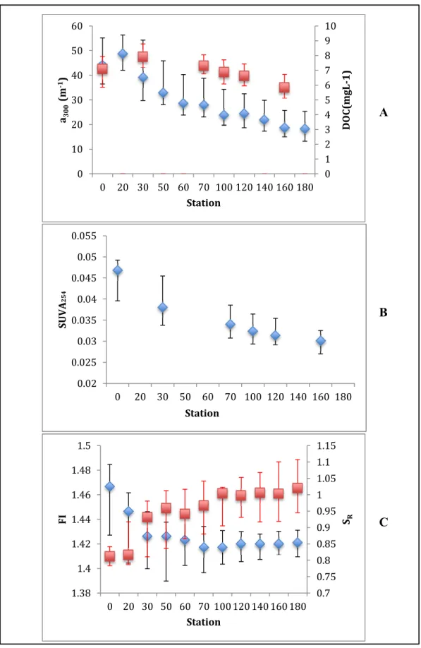
3.2 DOC, CDOM and FDOM variability along transect
Spatial and Temporal Trends
DOC concentrations ranged from 4.4 to 13.3 mg C L-1 over the study period (Table
(median = 7.9 mg C L-1), which is just downstream of the city of New Bern’s wastewater
treatment plant (Figure 3.2 A). Median DOC concentration decreased by approximately 27%
(6.0 mg C L-1) between upstream station 30 and downstream station 160. DOC
concentrations were highest during the winter and spring, and lowest during the fall and
summer (Appendix Figure 2 E).
Consistent with DOC concentrations, the absorbance coefficient (a300, m-1), a measure
of CDOM concentration, generally decreased downstream with values ranging from 10.7 -
84.6 m-1 over the course of the study (Figure 3.2 A; Table 3.1). Median a300 peaked at station
20 and increased by 9% between stations 0 and 20 and then decreased by 62% between
station 20 and 180. Seasonal patterns in a300 followed DOC concentration, with greatest
values and variation during the winter and spring seasons (Appendix Figure 2 F).
Consistent with the greater decrease in absorbance coefficient compared to the
decrease in DOC concentration with distance downstream, SUVA254, a proxy for aromatic
carbon content, also decreased along the downstream gradient (Figure 3.2 B). SUVA254
values ranged between 0.020 and 0.056 L mg-C-1 m-1 (Table 3.1). The largest median SUVA254 value was observed at station 0 at 0.047 L mg-C-1 m-1. Along the downstream gradient, median SUVA254 values decreased by 36% from stations 0 to 160. The magnitude
and variability in SUVA254 were greatest during the spring and winter months similar to DOC
and a300 (Appendix Figure 2 G).
Median values of the spectral slope ratio (SR), a CDOM proxy inversely correlated
17
3.1). The lowest median value of 0.81 and lowest variability in SR were observed at
freshwater station 0. SR was consistently highest at the downstream end-member station 180,
the most seawater station, with a median value of 1.02. The largest difference in median SR
between any two stations was observed between stations 20 and 30, where median values
increased by 15%. Lowest SR values, which indicate larger average molecular weight, were
observed during the winter and spring when DOC, a300, and SUVA254 measurements were
largest (Appendix Figure 2 H).
Median fluorescence index (FI) values ranged from 1.42 to 1.47, suggesting a mixed
source of allochthonous and autochthonous DOM (McKnight et al. 2001) (Table 3.1). The
median FI decreased from 1.47 to 1.42 between stations 0 and 30, whereas median FI values
did not vary significantly from station 50 to downstream station 180 (1.41 to 1.43) (Figure
3.2 C). The variability in FI was largest at the most upstream station 0 and lowest at the most
downstream stations 160 and 180 (Figure 3.2 C). Variability in FI at any station was lowest
in the spring, and highest in the summer (Appendix Figure 2 I).
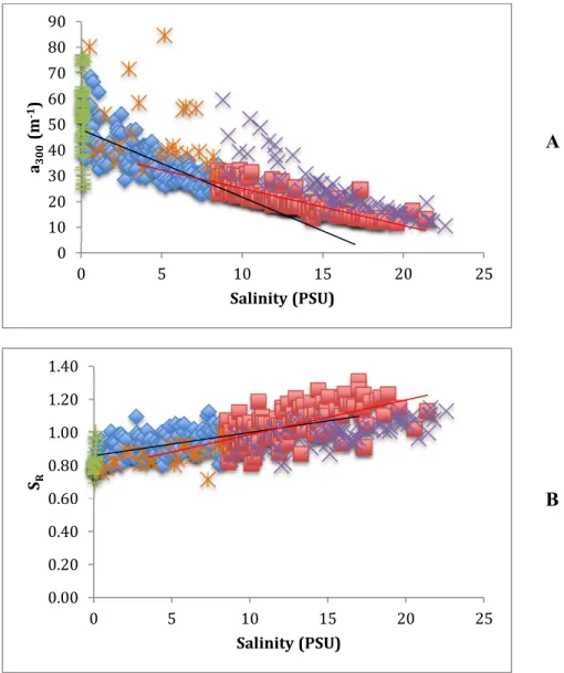
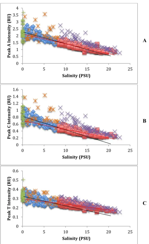
Trends with Salinity
While levels of CDOM and FDOM generally decreased with salinity in the NRE,
CDOM and FDOM exhibited different relationships with salinity depending on the salinity
range and sample date (Figure 3.3 A). For example, there was no relationship between a300
and salinity at low salinities (e.g. samples <0.27 PSU, Figure 3.3 A). Because a300 did not
decrease linearly with salinity across the entire range of observed salinities, samples were
split into two separate datasets at the median salinity value of 8.5 PSU. The slope of a300 vs.
high salinity samples (≥8.5 PSU) (m = -2.63 ± 0.40, p<0.05, R2 = 0.56; and m = -1.43 ± 0.17,
p<0.05, R2 = 0.67; low and high salinity datasets, respectively; Figure 3.3 A, Table 3.2).
Across the whole salinity range, samples collected on sampling dates in October-January
(2009-2010) and October 2010 had much higher a300 compared to most other samples. In
addition, there was no relationship between a300 and salinity for the subset of these samples
with salinity < 8.5 PSU, while the subset of these high a300 samples with salinity ≥8.5 PSU
exhibited a steeper slope compared to other ≥8.5 PSU samples (Figure 3.3 A). Thus, these
samples collected from October-January (2009-2010) and October 2010 were considered to
be outliers and not included in the linear fits for a300 vs. salinity.
Slope ratio (SR) against salinity exhibited weak positive linear relationships and no
significant differences were observed between the slopes of the low and high salinity datasets
(Figure 3.3 B, Table 3.2). The previously identified outlier samples collected in
October-January with higher a300, had lower SR values (Figure 3.3 B), but the relationship between SR
and salinity for these outlier samples was the same as the whole dataset.
Regressions of fluorescence intensities against salinity for humic EEM peaks A and C
(Coble 1996) revealed similar relationships to a300 vs. salinity. Intensities of peaks A and C
linearly decreased with increasing salinity, with significantly greater slopes in the low
salinity dataset than the high salinity dataset for peak C but not peak A (Figure 3.4 A & B;
slopes summarized in Table 3.2). As observed for a300 regressions, the previously identified
fall-winter outlier samples had higher peak A and C intensities, and these samples showed
different relationships with salinity compared to the whole dataset. For both the low and
19
Regressions between peak T intensity and salinity also exhibited a linear decrease
with increasing salinity similar to the peak A and C intensities. However there were
differences in the slope and distribution of the regression compared to the peak A and C
against salinity regressions (Figure 3.4 C; Table 3.2). For both low and high salinity datasets,
the slopes of the peak T vs. salinity regressions were significantly less than peak A and C
slopes by a factor of eight to 10 and three to four, for peak A and C regression slopes
respectively (Table 3.2). The previously identified fall-winter outlier samples did not exhibit
as large of a difference in intensity from the rest of the dataset as compared to the A and C
peak intensities (Figure 3.4 C). Although the T peak vs. salinity regression for these outlier
dates did not exhibit as large of an intensity difference as seen in the A and C peak
regressions, the regression slope of the ≥8.5 PSU outlier dataset was still significantly greater
than the high salinity dataset regression slope (data not shown).
Depth Trends
Differences in CDOM and FDOM between surface and bottom waters were related to
stratification in the water column at a given station. The difference in salinity between
depths (∆Salinity, defined as bottom minus surface water salinity) at any station along the
transect ranged from a minimum of 0 PSU (at station 0) to a maximum of 13.5 PSU (at
station 30), where salinity was always greater in the bottom water compared to surface water.
Generally, stations towards the freshwater and seawater end-members (stations 0, 20, and
180) had smaller depth differences in salinity compared to mid-stations, where average
∆Salinity was 3.7 PSU. Variations in the magnitudes and spatial extent of salinity
example, on 14-Jan, 2010 when the water column was highly stratified, mean ∆Salinity with
respect to depth along the entire transect was 10.8 PSU; whereas on the 28-Apr, 2010 when
the estuary was well-mixed, mean ∆Salinity was <1 PSU (data not shown).
For most samples, the lower salinity surface waters had greater a300 values than higher
salinity bottom water. For example, on the highly stratified date, 18-Oct, 2010, the low
salinity surface water had more than twice the CDOM (a300) than the bottom water
(Appendix Figure 3 A). Samples showing the opposite pattern, with higher CDOM in in
bottom waters compared to surface waters, were collected under well-mixed conditions when
depth differences in salinity were small (e.g. most of these samples had ∆Salinity < 1 PSU).
Generally, the percent difference in CDOM (a300) with respect to depth (calculated as surface
minus bottom a300) was positively correlated with the depth ∆Salinity (m= 4.04 ± 0.48,
p<0.05, R2= 0.57) (Figure 3.5 A).
Trends in percent difference in FDOM peaks A, C, and T with respect to depth were
similar to percent change in CDOM with depth (Figure 3.5 B, C, and D). Intensities of all
FDOM peaks were generally greater in the surface than in bottom water. Similarly to
CDOM, deviation from this trend primarily occurred under well-mixed conditions when
depth differences in salinity were small (<3 PSU). Generally, depth difference in the percent
change in A, C, and T intensity (calculated as surface minus bottom intensity) had a positive
relationship with ∆Salinity, with slightly greater slopes for peaks A and C compared to peak
T (m= 3.14 ± 0.40, p<0.05, R2= 0.53; m= 3.81 ± 0.42, p<0.05, R2= 0.60; m= 2.38 ± 0.31,
21 3.3 PARAFAC modeling and validation
Attempts at modeling the NRE resulted in to two independent PARAFAC models
split by salinity. Preliminary attempts to validate greater than two components from a
whole-system PARAFAC model for the NRE failed due to the inherent variability of the fluorescent
signatures along the entire freshwater to seawater continuum. With two components
validated, clear peaks were present in residual EEMs (data not shown), demonstrating that a
‘whole system’ model did not describe all the underlying variability of FDOM in the NRE.
Based on the different slopes observed for CDOM and FDOM vs. salinity, two independent
PARAFAC models were tested by splitting the whole dataset into two subsets based on the
criterion of whether the sample was above or below the median salinity value of 8.5 PSU.
This approach resulted in validation of three FDOM components from each model, where the
final validated models consisted of 445 and 418 EEMs for the <8.5 and ≥8.5 PSU models
respectively—with 31 and 25 EEMs removed as outliers respectively. Three components
were validated for each model by four-way split-half validation—F1, F2, and F3 are the
freshwater (F) components for the <8.5 PSU model and S1, S2, and S3 are the seawater (S)
components for the ≥8.5 PSU model; where the order of the validated components in each
model corresponds to the amount of variation each component explained in the dataset of
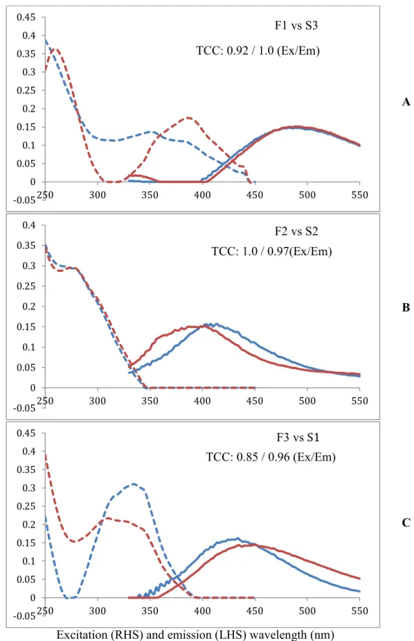
EEMs. (Figure 3.6; Table 3.3).
F1 was found to have a good degree of similarity to S3, based on a TCC value of 0.92
and 1.0 for excitation and emission spectra respectively (Figure 3.7 A). F2 and S2 were
found to be equivalent at a congruence value of 1.0 and 0.97 (for excitation and emission
spectra respectively) (Figure 3.7 B). The emission peak position for F3 was blue-shifted
determined to have a good degree of similarity by the TCC at a congruence level of 0.96.
The excitation spectra of F3 and S1 were statistically different at a congruence of 0.85,
meaning that these components are distinct from one another (Figure 3.7 C). F3 and S1 had
the same primary excitation peak at <250 nm but different secondary excitation maxima of
335 nm and 310 nm respectively (Table 3.3).
Because the TCC test is not a completely definitive measure of congruence for
PARAFAC components derived from different models, an additional cross comparison of
components was tested by fitting each dataset to the opposing PARFAC model. Samples
from the low salinity dataset were fitted to the ≥8.5 PSU model and the corresponding
component Fmax, values were compared to the Fmax, values from the < 8.5 PSU model (and vice versa for samples from the high salinity dataset fit to the < 8.5 PSU model). The Fmax values from the two models for the three corresponding components were linearly related
with correlation coefficients (R2) ranging from 0.72 to 0.99 (Table 3.4). Fmax values of the low salinity dataset fit to the ≥8.5 PSU model were twofold lower for the humic terrestrial
(S3) and marine humic (S2) components, with slopes of 0.5 (Table 3.4), indicating that 50%
of the fluorescence assigned to these components in the < 8.5 PSU model was assigned to the
S1 component of the ≥8.5 PSU model. Consistently, Fmax values of the low salinity dataset that were fit to the ≥8.5 PSU model were about 2.4 times higher for the humic terrestrial (S1)
component. Conversely, the high salinity dataset fit to the < 8.5 PSU model always
produced twofold more loading for the humic terrestrial component (F1) and marine humic
component (F2) compared to the corresponding components in the original ≥8.5 PSU model
23
models tended to predict loadings in favor of the order of their respective components. For
example, for the same sample fit to both models, the loading of the humic terrestrial
component (F1) was greatest in the <8.5 model as F1, but the same sample fit to the ≥8.5
model had the lowest loading in corresponding humic terrestrial component as S3.
The regression coefficients between the fitted and original loadings show that
component loadings were not consistently quantified between corresponding components in
the two models. R2 values of the regression coefficients between fitted and original loadings
were lower when the low salinity dataset was fitted to the ≥8.5 PSU model than when the
high salinity dataset was fitted to the <8.5 PSU model (Table 3.4). R2 values were high
(≥0.93) for the fitted vs. original loadings of the terrestrial humic and humic components in
both model fits (Table 3.4). The marine humic component had lower R2 values (0.72 and
0.86, for low salinity fitted to ≥8.5 PSU model and vice versa, respectively), showing that the
variability of this component in one model was not as well explained by the variability in the
opposite model. Comparing the emission spectrum between the two marine humic
components (F2 and S2), it is clear that the S2 component is modeling additional
fluorescence in the amino acid peak region (Ex/Em 280/350nm) that is not captured by
IV. DISCUSSION
4.1 Spatial and temporal patterns
Changes in the quantity and quality of DOM, as evidenced by analysis of DOC,
CDOM, and FDOM along the freshwater to seawater transect in the NRE, were similar to
other investigations of DOM along freshwater to estuarine gradients—suggesting that similar
biogeochemical controls may influence the source and fate of DOM across different estuarine
systems. Based on the spatial and temporal patterns of DOC concentrations and CDOM and
FDOM quality in the NRE, upstream terrestrial sources of DOM were found to be the major
sources of DOM, which was consistent with other estuarine systems (Stedmon and Markager
2005a, 2005b, Yamashita et al. 2008, Murphy et al. 2008, Kowalczuk et al. 2009, Singh et al.
2010, Fellman et al. 2011, Guo et al. 2011). Highest DOC and CDOM toward the upstream
end-member and a linear decrease in DOC and CDOM abundance with respect to salinity
indicated that most of the DOM loading from the estuary was from upstream terrestrial inputs.
Additionally, analysis of CDOM quality based on SR and SUVA254 showed that the upstream
end-member sources of DOM had greater average molecular weight and aromaticity,
consistent with terrestrial sources of DOM enriched in large aromatic ring structures
(McKnight et al. 2003). Seasonal patterns in DOC and CDOM further reinforced the
importance of terrestrial carbon sources to the NRE, based on the fact that the highest CDOM
with the highest average molecular weight and aromaticity (characteristic of terrestrial DOM)
25
pool were during periods of high discharge was consistent with the findings in Peierls and
Paerl (2010), showing that DOC input and concentrations in the NRE correlated with
seasonal patterns of discharge. Taken together, these results underscore the large contribution
of upstream terrestrial inputs to the DOM pool of the NRE.
Given the importance of terrestrial DOM to the NRE, it is critical to understand how
its chemical composition is altered as it is transported downstream. We found that average
molecular weight and aromaticity decreased long the freshwater to seawater gradient in the
NRE, consistent with the findings in the Helms et al. (2008) study of the Chesapeake Bay, an
Atlantic coast estuary that is similar in climate to the NRE, and other studies (Vahatalo et al.
2005, Gonsior et al. 2009, Kowalczuk et al. 2009). Shifts in the quality of
terrestrially-derived CDOM as it is transported downstream are likely due to a mixing with the seawater
end-member as well as processes that remove terrestrial DOM, such as coupled
photochemical and biochemical degradation (Boyd 2004, Gonsior et al. 2009) along with
flocculation and sedimentation (Sholkovitz 1976). The chemical quality of the seawater
‘end-member’ DOM was inferred from the quality of DOM at the most downstream stations
160 and 180 where DOC concentration was lowest. DOM at stations 160 and 180 exhibited
the lowest average molecular weight and aromaticity. Mixing of low DOC seawater of lower
molecular weight and aromaticity with high DOC upstream water of higher molecular weight
and aromaticity derived from terrestrial sources is consistent with the general pattern of
decreasing DOC, molecular weight, and aromaticity of the DOM with distance downstream
in the NRE. However, removal processes such as photochemical degradation and
sedimentation also decrease the molecular weight and aromaticity of the DOM (Helms et al.
result in the degradation of terrestrial DOM are also likely to contribute to the shifts in DOM
quantity and quality in the NRE.
4.2 Hydrological regime influence on CDOM and FDOM dynamics
CDOM and FDOM measures have often been utilized in studies along a freshwater to
seawater continuum to explain the chemical phenomena underlying the distribution and
character of organic matter chromophores (Clark et al. 2002, Stedmon and Markager 2005a,
Stephens and Minor 2010). I chose to present the spatial analysis of data with respect to
change in salinity in respect to depth because the change in salinity provided a representation
of the variable mixing dynamics of the system.
In this study the widely accepted convention of classifing FDOM EEM spectra into
the ubiquitously identified peaks A, C and T was utilized. Peaks A and C are attributed to
the humic or fulvic fraction of DOM, with Peak A exhibiting excitation/emission (Ex/Em)
maxima in the region of 260/380-450. nm and peak C exhibiting maxima at Ex/Em=
312/380-450 nm (Coble 1996). Peak T has been associated with proteinaceous
compounds—more specifically with the fluorescence of tryptophan-like compounds (Coble
1996)—due to the fact that it exhibits excitation/emission maxima very similar to tryptophan
(Ex/Em = 250-285/344 nm).
The positive relationship of the percent changes in peaks A, C, and T with change in
salinity in respect to depth indicated that during stratified conditions surface waters were
enriched with humic and tryptophan-like FDOM compared to bottom waters (Figure 3.5 C, D,
27
CDOM under stratified conditions compared to bottom waters (Figure 3.5 A). The classic
estuarine hydrodynamic regime creates a bidirectional flow where surface waters flow
downstream and bottom waters flow upstream ( Leuttich et al., 2001); and thereby creates a
stratified water column with contributions from the freshwater end-member at the surface
and the seawater end-member near the bottom. In a paper describing the NRE
hydrodynamics by Luettich et al. (2001), it was determined from one year of weekly
sampling that the estuary experienced classic estuarine flow 52% of the time. Because
surface waters are associated with the freshwater end-member under stratified conditions, the
greater CDOM and FDOM in surface waters relative to bottom waters further highlights the
importance of terrestrial sources of CDOM and FDOM that are washed in with freshwater
discharge from the watershed into the NRE (Stedmon and Markager 2005a, Murphy et al.
2008).
While it is clear that overall levels of FDOM were higher in surface waters compared
to bottom waters, the differences in regression slopes between the percent change of the three
types of FDOM (peaks A, C and T) with change in salinity in respect to depth indicates that
there are differences in the distribution of humic and protein-like FDOM under stratified
conditions (Table 3.2). The percent change in humic peaks A and C in respect to depth had a
significantly greater slope than the percent change in protein-like peak T, indicating a greater
difference in peaks A and C between the more freshwater surface water and more saline
bottom water than peak T. Because surface waters are more associated with the freshwater
end-member, the difference between the slopes of the A and C peaks compared to the T peak,
protein-like material derived from microbial sources. This result may suggest a source of
protein-like FDOM from sediments.
The variation observed in regressions between percent change in peak intensity and
change in salinity in respect to depth may be explained by the seasonal differences in DOM
loading. Samples identified as outliers due to their higher CDOM (a300 values) relative to the
rest of the dataset were collected during periods known to experience increased leaf litter
input and high discharge volumes (fall and winter dates 29-Oct 2009, 9-Nov 2009, 1-Dec
2009, 14-Jan 2010, and 18-Oct 2010), which likely introduced large quantities of CDOM and
FDOM from the watershed. In the percent change in peak A, C, and T intensity with change
in salinity regressions, these dates showed greater percent change in peak intensity under
stratified conditions when compared to other sampling dates. Given the variations in water
column mixing and seasonal loadings, it is evident that CDOM dynamics in the NRE are
strongly coupled to the variable hydrodynamics of the system.
4.3 Impact of salinity on CDOM
Differences between a300 measurements between low salinity and high salinity
datasets may suggest different rates of CDOM processing (removal or production) or the
physicochemical effects of salinity. The effects of salinity on the light absorption and
photochemical properties of CDOM has been often studied but with contrasting results,
which may in part be due to different metrics used to define photoactivity (Hu et al. 2002).
Osburn et al. (2009) studied the effects of salinity on CDOM photobleaching and
demonstrated that chromophores contributing to the high CDOM absorbance in the low
29
nm) were found to be affected by salinity. Findings from the Osburn et al. (2009) study
tentatively suggest that our measure of CDOM at 300 nm in this study (e.g. a300 ) may not
have been affected by salinity. If this assumption is correct, then the observed differences in
the slope of CDOM vs. salinity between the low and high salinity datasets are likely due to
differences in biogeochemical processes modifying DOM along the salinity gradient, such as
photodegradation (Del Vecchio and Blough 2002, Vahatalo et al. 2005), flocculation of high
molecular weight DOM (Sholkovitz 1976), microbial uptake (Amon and Benner 1996), or
differential mixing and dilution patterns.
In this study, differences in the regression of the slope ratio (SR) with salinity between
low and high salinity datasets were not significant, indicating that the molecular weight
varied consistently with salinity among the two datasets. Contrasts between the SR and a300
results among the datasets suggest that the relative changes in the chromophores absorbing at
low and high wavelength were similar along the salinity gradient.
The analysis of CDOM concentrations in the NRE does not provide a clear
assessment of relative importance of mixing vs. degradation of DOM as it is transported
downstream. This is because DOM is a diverse collection of organic molecules that exhibit
different residence times and turnover rates not detectable with bulk concentration measures
(Kaplan et al. 2008). Increasingly, analysis of the fluorescent fraction of DOM (FDOM) by
parallel factor analysis (PARAFAC) of excitation emission matrices (EEMs) is proposed as
an approach to trace the dynamics of these different fractions of DOM at a finer scale than
provided by DOC or CDOM. However, results from this study show that are there
salinity gradients such as those that exist in the NRE, likely due in part to the effects of
salinity on FDOM signals.
4.4 Impact of salinity on FDOM: EEM peak picking
Like CDOM, different relationships of FDOM and salinity among the low and high
salinity datasets may suggest differences in the biogeochemical processes controlling FDOM
in these waters. Alternatively, there may be direct physicochemical effects of salinity on
FDOM signals due to changes in ionic strength that alter the local chemical environment
around the fluorescing moiety. Given that fluorescence is much more sensitive to the local
chemical environment than absorbance (Lakowicz 1999), it is likely that FDOM signals may
be influenced by differences in salinity, as suggested previously by other studies (Mobed et
al. 1996, Clark et al. 2002, Minor et al. 2006, Boyd et al. 2010).
Other factors influencing fluorescence intensity include the concentration of the
fluorescing moiety (e.g. fluorophore concentration). For example, decreasing fluorescence
intensity corresponding to decreasing fluorophores concentration may be attributed to mixing
and dilution independent of physicochemical changes of salinity effects. Biological and
physical removal processes may also be attributed to decreases in fluorophore concentrations.
However some of this observed removal may actually be due to decrease in fluorescence
intensity due to change in the molecular environment/conformation of DOM with increasing
salinity. Recently, it was found that increasing salinity facilitated molecular changes in
conformation with certain types of humic CDOM molecules (Batchelli et al. 2009). This
kind of change in the conformation of humic CDOM with salinity has been attributed to
31
2004). Additionally, the process of flocculation of humic substances in estuaries has been
demonstrated to be highly dependent on salinity by the occurance of rapid flocculation of
river DOM when introduced to marine water (Sholkovitz 1976).
Boyd et al. (2010) showed relatively constant fluorescence intensity for humic peak A
of selected size fractions of DOM sampled from different estuaries as a function of
laboratory-simulated salinity increments. In contrast, these same samples amended with salt
exhibited variability in humic peak C intensity as a function of salinity. Results from our
study support the findings of Boyd et al. (2010) showing that different fractions of FDOM
vary in their apparent susceptibility to influences of salinity. Consistent with results from
Boyd et al. (2010), the slope of peak A intensity vs. salinity in the NRE did not differ
between the low and high salinity datasets. This contrasted to the slopes of the intensities of
peaks C and T vs. salinity, which did differ among low and high salinity datasets.
The observed decrease in the fluorescence index (FI) along the salinity gradient in the
NRE also suggests an influence of salinity on FDOM signals. A decreasing FI suggests
greater proportion of terrestrially derived DOM in the total DOM pool at the most
downstream stations, which is opposite of what is expected based on the patterns in DOC,
CDOM and other FDOM analyses. The FI of a given sample decreases with exposure to
sunlight due to photodegradation of the DOM (Cory et al. 2007). Thus it is possible that a
decrease in FI with distance downstream is due to photodegradation of the DOM as it is
transported downstream. Loss of CDOM (a300) and fluorescence intensities along with an
increase in SR are all consistent with the photochemical degradation of DOM (Stedmon and
However, others have reported that salinity may alter the chemical properties of the
fluorophores contributing to the FI. For example, Boyd et al. (2010) found that under
simulated estuarine salinity transects, increasing salinity can cause a decrease in the FI of the
DOM sample, consistent with this study showing decreasing FI with increasing salinity in the
NRE. Interestingly, Boyd et al. (2010) reported that the effect of simulated salinity on the FI
depended on the source and size fraction of DOM, e.g. whether the DOM was collected from
upstream or downstream end-members. Other studies that have traced FI values along
freshwater to seawater gradients have reported mixed trends, with some studies showing the
expected decrease in FI with increasing salinity—indicating a shift from terrestrial to
microbial carbon sources in the DOM pool (Jaffé et al. 2004, Stedmon and Markager 2005a,
Singh et al. 2010)—while others did not show any pattern with increasing salinity (Murphy
et al. 2008). Collectively, these results strongly suggest that salinity may have a chemical
effect on the fluorescent moieties that contribute to the FI, and that this effect likely depends
on the source and chemistry of the DOM. The chemical effect of salinity further complicates
the use of the FI to trace DOM sources across salinity gradients.
4.5 Effect of salinity on FDOM: PARAFAC
The analysis of the intensities of major EEM peaks A, C and T or of ratios of
intensities (such as the FI), each calculated at fixed excitation and emission wavelengths, do
not provide any information about the shifts in the underlying spectra contributing to
fluorescence intensity at any specific excitation/emission pair. Because it is expected that
chemical changes in DOM due to salinity would cause a shift in both the quantum yield
33
PARAFAC among the low and high salinity datasets may provide more insight into the
effects of salinity on FDOM signals.
PARAFAC has been utilized in several estuarine, coastal, and marine studies to trace
sources and reactivity of different FDOM fluorophores (Stedmon and Markager 2005,
Murphy et al. 2008, Singh et al. 2010, Gao et al. 2011). However in contrast to these studies,
we were unable to validate a unified PARAFAC model for the total dataset of samples
collected along the transect of the NRE. Inability to validate a unified model for the whole
system compared is likely due to the stricter four-way split-half validation method employed
in our study, which revealed that there were unresolvable differences in fluorescence
signatures along the freshwater to seawater salinity gradient.
Component descriptions and proposed source
Two independent PARAFAC models were validated composed of samples in the low
or high salinity datasets, and these models resulted in very similar, but not identical
components. The components derived from the NRE models were very similar to
components identified from many previous studies of both freshwater and estuarine systems
(Table 3.3). F1 and S3 are ubiquitous fluorophores that contribute to the identified A and C
peaks of humic-like terrestrial material (Coble 1996). Humic-like material with similar
properties to F1 and S3 have been linked to terrestrially-derived material that have optical
properties of degraded lignin (Del Vecchio and Blough 2004, Boyle et al. 2009). The
emission-excitation spectra of F2 and S2 correspond to the “marine” humic peak M (Coble
1996), which is generally thought to be derived from autochthonous sources. Peak M has
have shown a strong correlation between peak M with terrestrial humic fluorescence; and
thus it is currently less accepted as a tracer for marine end-member DOM (Stedmon et al.
2003, Murphy et al. 2008). Despite the increasing evidence that the peak M is ubiquitously
present in freshwater and marine systems, the F2 and S2 components are referred to as
“marine humic” in this study, as is the convention. The S2 component also partially captured
fluorescence of amino acid-like fluorophores given that there was appreciable emission at
350 nm varying linearly with the marine peak M; thus in the ≥8.5 PSU model S2 may
provide insight on the amino acid fraction of FDOM.
Of the three pairs of components, F3 and S1 were the least similar (as tested by the
Tucker Convergence Criteria test). F1 and S3, also comprise humic peaks A and C.
Components similar to F3 and S1 have been ubiquitously identified in many systems and
thus F3 and S1 are referred to as “humic” components in this study. These component
source assignments are necessarily broad because the complex solutions of natural waters
contain many emitting species that make the definitive classification of fluorescing
constituents difficult.
The order of derived components in our models revealed that a greater fraction of the
total fluorescence in the low salinity dataset was explained by the terrestrial humic
component F1, whereas in the high salinity dataset the analogous component (S3) explained
the least amount of variation in the total fluorescence (given that it was the third of three
components to be validated). This result also supports the importance of terrestrial sources
of humic CDOM and FDOM of upstream origin in the NRE. The lower importance of the
35
flocculation and precipitation of humic materials as a result of mixing with high salinity
water (Sholkovitz 1976).
In contrast to the terrestrial humic component, the humic component (F3 or S1,
depending on the model) showed the opposite pattern. The humic component explained the
least variability in the low salinity samples (identified as the third of three components, e.g.
F3), whereas it explained the most variability in the high salinity samples (e.g. identified as
the first component, S1). A study by Batchelli et al. (2009) demonstrated that LMW humic
FDOM with similar emission maxima as F3 and S1 may have undergone conformational
changes upon mixing with the seawater end-member. This finding may suggest that F3 and
S1 may differ due to significant physicochemical changes induced by salinity that may alter
the fluorescence spectra of similar compounds in different chemical environments.
The marine humic component remained relatively consistent in its contribution to the
FDOM pool between both models as F2 and S2, supporting the findings that the marine
humic component is common to both freshwater and marine environments. It is ultimately
unclear whether removal production/processes or physicochemical effects are influencing the
relative importance of components within each dataset, though it is certain that there are
differences between the two datasets. Further examination of the fluorescence spectra of the
components may provide further insight upon the differences in the models.
Examination of component excitation and emission spectra
As expected, results from PARAFAC modeling demonstrated differences in the
FDOM spectra between the high and low salinity datasets, which may be due to effects of
shows that there was high variability in the underlying fluorescence spectra of DOM along
the salinity gradient, which in turn suggests that salinity alters the chemical properties of the
fluorescing moieties in the DOM pool, such that their quantum yields and excitation and
emission spectra may shift due to differences in the local molecular environment as a
function of ionic strength. Such effects could include quenching by inorganic species and/or
conformational shifts in the fluorescent moieties brought about by differences in ionic
strength, interactions with inorganic species, or by differences in polarity.
For the marine humic components (F2 and S2), the S2 emission maxima was
blue-shifted (blue-shifted toward shorter wavelength) relative to F2 (Figure 3.7). The blue-shifting of
the S2 modeled in the ≥8.5 PSU model is consistent with other studies (Kowalczuk et al.
2009, Boyd et al. 2010), suggesting that the fluorescent signatures of different types of DOM
may shift towards shorter wavelength peak positions along a salinity gradient. A
blue-shift of DOM emission peak position towards shorter wavelengths along salinity gradients
has been attributed to a decrease in solvent polarity in seawater (Lakowicz 1999). This
decrease in polarity surrounding the fluorescing moiety in seawater may be due to salt ion
interaction with dipoles of water molecules or due to decreasing hydrophobic interactions
facilitated by aromatic molecules enriched in terrestrial DOM compared to marine DOM.
In contrast to the expected differences between freshwater and seawater FDOM, the
humic component S1 was red shifted to longer wavelength compared to its analogous
component in the freshwater model (F3). Red shifting has been suggested to occur in humic
compounds due to the formation of colloidal assemblages due to ionic effects along the