ASSESSMENT OF AIRCRAFT EMISSIONS IMPACTS ON AIR QUALITY AT MULTIPLE 1
MODEL SCALES 2
Lakshmi Pradeepa Vennam 3
A dissertation submitted to the faculty at the University of North Carolina at Chapel Hill in 4
partial fulfillment of the requirements for the degree of Doctor of Philosophy in the Department 5
of Environmental Sciences and Engineering in the Gillings School of Global Public Health. 6
Chapel Hill 7
2016 8
Approved by: 9
Saravanan Arunachalam 10
William Vizuete 11
Rohit Mathur 12
Jason West 13
1 2 3 4 5 6 7 8 9 10 11 12 13 14 15 16 17 18 19 20 21 22 23 24 25 26 27 28 29 30 31 32 33 34 35 36 37 38 39 40
© 2016 41
Lakshmi Pradeepa Vennam 42
ALL RIGHTS RESERVED 43
1
ABSTRACT 2
3
Lakshmi Pradeepa Vennam: Assessment of aircraft emissions impacts on air quality at multiple 4
model scales 5
(Under the direction of Saravanan Arunachalam and William Vizuete) 6
7
Aviation activity has grown steadily, and will likely continue to grow in the future. 8
Aviation-related air pollutants occurring during full-flight (landing and takeoff, as well as cruise) 9
can impact air quality, human health and climate. The overall goal of this dissertation is to study 10
the air quality impacts of aviation at local, regional and global scales. The central hypothesis of 11
this study is that fine scale modeling provides better characterization of aviation emissions 12
impacts on air quality and health. To test this hypothesis, a model-based assessment of aviation 13
emissions impacts was conducted at multiple scales ranging from local (4 × 4 km2) to 14
hemispheric (108 × 108 km2) scales. 15
Firstly, we focused on key risk-prioritized Hazardous Air Pollutants (HAPs) and assessed 16
their impacts near a mid-sized U.S. airport using a chemistry-transport model at a fine scale (4 × 17
4 km2). Overall modeled aircraft-attributable HAPs contributions are in the range of 0.5 – 28% 18
near this airport. Second, we concentrated on the full-flight emissions impacts on air quality near 19
surface for O3 and PM2.5 at a resolution of 108 × 108 km2, spanning the Northern hemisphere 20
(NH). Including full-flight aviation emissions at the hemispheric scale contributed 1.3% and 21
0.2% for O3 and PM2.5 at the surface on an annual domain-wide basis. Our comparison of these 22
predictions with 36 × 36 km2 application over North America highlighted that the coarse scale 23
resolution was unable to capture non-linearities in chemical processes near airport locations and 24
processes on cruise altitude aviation emissions (CAAE) impacts at the surface using a 1
hemispheric scale application. Model predictions indicated that < 0.6% of CAAE tracer in the 2
total atmospheric column was transported to the surface and ~40% was transported to mid- 3
troposphere during all four seasons. This intercontinental tracer-tagging approach provided 4
quantitative evidence that North America and Europe CAAE tracers can impact the surface (~0.5 5
– 1% of total column burden) near high terrain regions like Tibet Plateau and relatively lower 6
aviation emissions regions such as Middle East, North Africa and South East Asia. 7
1
ACKNOWLEDGEMENTS 2
Firstly I am very grateful to my advisors: Dr. Saravanan Arunachalam and Dr. William 3
Vizuete for their support, patience, cooperation throughout my PhD coursework and research. I 4
owe my appreciation and deepest gratitude to them. My sincere thanks to Sarav for the financial 5
support during all these years under Federal Aviation Administration project funding. I would 6
also like to acknowledge my committee members for being in my committee and for their 7
valuable suggestions. 8
A simple thanks is very less to my family and friends who gave enormous support 9
throughout my graduate school. Without my Father (V. Naga Malleswara Rao), Mother (V. 10
Padmavathi) and Sister (V.L. Praneetha), I wouldn’t have been in this position today. My 11
husband (P.V Ravi Kiran) has been my biggest support and immense strength throughout my 12
graduate school (Masters and PhD) period since 2008 and motivated me from time to time. Since 13
I got married last year (2015) my in-laws are very supportive and helped me focus on my 14
research. Last but not the least my friends in Chapel Hill area are very friendly, helpful, 15
supportive and gave me some social life during weekends. 16
I want to thank my IE lab mates: Matt, Changsy, and Scott for their wonderful company, 17
more than lab mates they are like my brothers. We shared lot of technical discussions, 18
programming skills and having them around made a huge difference in acquiring knowledge. I 19
want to thank my colleagues at Institute for the Environment (Jeanne (retired), Frank, BH, 20
1
TABLE OF CONTENTS 2
LIST OF TABLES ... ix 3
LIST OF FIGURES ... xii 4
CHAPTER 1: INTRODUCTION ... 1 5
CHAPTER 2: EVALUATION OF MODEL-PREDICTED HAZARDOUS AIR 6
POLLUTANTS NEAR A MID-SIZED U.S. AIRPORT ... 9 7
8
2.1 INTRODUCTION ... 9 9
10
2.2 METHODOLOGY ... 12 11
2.2.1 Air Quality Model (CMAQ) ... 12 12
2.2.2 Observational Data ... 16 13
2.2.3 HAPs estimates from NATA ... 17 14
15
2.3 RESULTS ... 18 16
2.3.1 Model Evaluation: 4 × 4 km2 grid resolution ... 18 17
2.3.2 Comparison of 4 × 4 km2 with 36 × 36 km2 ... 24 18
2.3.3 Sensitivity of Aircraft emissions ... 26 19
2.3.4 Comparison of 4 × 4 km2 with NATA estimates ... 29 20
21
2.4 FUTURE WORK AND CONCLUSIONS ... 31 22
23
2.5 ACKNOWLEDGEMENTS ... 33 24
CHAPTER 3: MODELED FULL-FLIGHT AIRCRAFT EMISSIONS IMPACTS 25
ON AIR QUALITY AND THEIR SENSITIVITY TO GRID RESOLUTION ... 34 26
27
3.1 INTRODUCTION ... 34 28
29
3.2 METHODOLOGY ... 39 30
3.2.2 Observation data ... 43 1
3.2.3 Mass Flux ... 44 2
3.2.4 Isentropic Analysis ... 44 3
4
3.3 RESULTS AND DISCUSSIONS ... 45 5
3.3.1 Aviation emissions impact at hemispheric scale ... 45 6
3.3.1a Surface Analysis ... 45 7
3.1.1b Vertical Analysis ... 51 8
3.3.2 Grid Resolution Sensitivity ... 58 9
3.3.2a Model Evaluation ... 58 10
3.3.2b Aviation impacts comparison ... 63 11
3.3.2c Emission Inventory Sensitivity ... 65 12
13
3.4 CONCLUSIONS ... 67 14
CHAPTER 4: TRACER STUDY TO ESTIMATE THE TRANSPORT OF 15
CRUISE ALTITUDE AVIATION EMISSIONS IN NORTHERN HEMISPHERE ... 70 16
17
4.1 INTRODUCTION ... 70 18
19
4.2 METHODOLOGY ... 74 20
4.2.1 Tracer Model ... 74 21
4.2.2 Model Inputs and Specifications ... 75 22
4.2.3 Analysis metrics ... 77 23
24
4.3 RESULTS ... 78 25
4.3.1 Tracer surface distribution ... 78 26
4.3.2 Tracer vertical distribution ... 81 27
4.3.3 Source-receptor distributions ... 84 28
29
4.4 CONCLUSIONS ... 89 30
APPENDIX A: SUPPLEMENTAL MATERIAL: EVALUATION OF MODEL 1
PREDICTED HAZARDOUS AIR POLLUTANTS (HAPS) NEAR A MID- 2
SIZED U.S. AIRPORT ... 98 3
4
APPENDIX B: SUPPLEMENTAL MATERIAL: MODELED FULL-FLIGHT 5
AIRCRAFT EMISSIONS IMPACTS ON AIR QUALITY AND THEIR 6
SENSITIVITY TO GRID RESOLUTION ... 117 7
REFERENCES ... 142 8
LIST OF TABLES 1 2
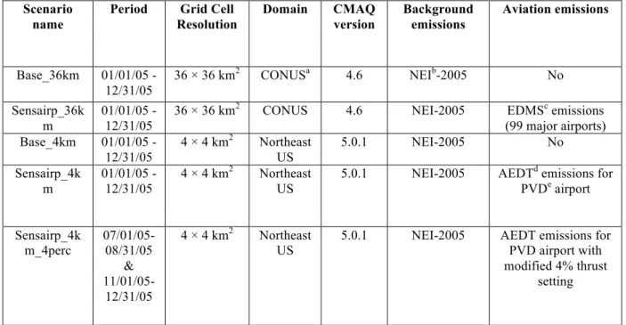
Table 2.1: Specifications and description of modeling scenarios in the study ... 13 3
4
Table 2.2: Annual NME (%, top) and NMB (%, bottom) using pollutant 5
predictions from the sensairp_4km averaged for all sites and differentiating 6
RIDEM and AQS sites. Also shown in parenthesis are the base_4km case 7
(with no airport emissions) values. ... 20 8
9
Table 2.3: Annual NME (%, top panel) and NMB (%, bottom panel) from all 10
sources at (36 × 36 km2) and (4 × 4 km2) cases at all sites and differentiating 11
between RIDEM and AQS sites ... 25 12
13
Table 2.4: Difference in NME [sensairp_4km (NME) minus sensairp_4km_4perc 14
(NME)] at the RIDEM sites for four months. ... 27 15
16
Table 2.5: Comparison of CMAQ (sensairp_4km) and NATA model with NME 17
(%, top panel) and NMB (%, bottom panel) values for all sites and 18
differentiating RIDEM, AQS sites. ... 30 19
20
Table 3.1: Modeling configuration and data sources for HEMI and CONUS 21
domains. ... 40 22
23
Table 3.2: Description of modeling scenarios ... 43 24
25
Table 3.3: Domain wide annual average of predicted O3 and PM2.5 aviation- 26
attributable contributions (AAC) for overall HEMI domain and the sub- 27
regions of NA, EU and EA. The relative percentage of aircraft emission 28
contribution when compared with all sources is shown in parenthesis. Also 29
shown are the maximum annual AAC in the domain for both pollutants. ... 47 30
31
Table 3.4: Seasonal Normalized Mean Bias (%) of hourly O3 and PM2.5 32
concentrations predicted by Airc36 and Airc108 model scenarios in 33
comparison with hourly AQS observations. All Airc108 predictions were 34
limited to the NA region. Also shown are the NME (%) differences 35
(Airc108 –Airc36) between scenarios. ... 59 36
37
Table 3.5: Normalized Mean Bias (%) metric of O3, NO2 and NO from three 38
model scenarios NoAirc36, Airc36, Airc108 in comparison with INTEX- 39
NA observations. Here we are showing the maximum, minimum and 40
average values of all altitudes (0 – 12km). Also shown are the Normalized 41
Mean Error (%) differences between Airc36 with NoAirc36, Airc108 model 42
scenarios. ... 61 43
Table 3.6: Domain-wide monthly average aviation-attributable contributions 1
(AAC) of O3 and PM2.5 from model scenarios a) Airc108-NoAirc108 2
(HEMI-NA) b) Airc108_NEI-NoAirc108_NEI (HEMI-NEI-NA) and c) 3
Airc36-NoAirc36 (CONUS). Also shown are the ratio comparisons of these 4
scenarios for January and July months. ... 65 5
6
Table 4.1: Domain wide averaged surface mass fraction percentage for each 7
season ... 79 8
9
Table 4.2: Tracer source-receptor contribution metric (Equation 4.2) for four 10
seasons of North America (NA), Europe (EU) and East Asia (EA) sources. ... 88 11
12
Table A1: Total Organic Gas (TOG) speciation profile of HAPs for aircraft 13
engines developed by EPA/FAA (EPA, 2009) ... 98 14
15
Table A2: Transport and chemical processes parameterizations used in CMAQ 16
v5.0.2 for the 4 × 4 km2 simulations. ... 99 17
18
Table A3: Monitoring sites and their description near PVD airport ... 100 19
20
Table A4: NATTS observation sites and airport grid-cells in 36 × 36 km2 21
domain. ... 101 22
23
Table A5: HAPs airport emission totals for 99 airport grid-cells in the sensairp_36 24
km case and PVD airport grid-cell in sensairp_4km case. Contributions of 25
these emissions to the total emissions (airport + background) are also 26
shown. ... 103 27
28
Table A7: Comparison of 36 × 36 km2 (from EDMS) and 4 × 4 km2 (from 29
AEDT) PVD grid cell airport emissions. ... 104 30
31
Table A8: Predicted airport contribution in winter (January) and summer (July) 32
months to the ambient concentrations in 4 × 4 km2 PVD airport grid-cell. ... 111 33
34
Table B1. Domain specifications used in WRF for CONUS and HEMI domains ... 117 35
36
Table B2: Vertical structure used in WRF meteorology modeling for two domains ... 118 37
38
Table B3: Physical meteorology parameterization options used in WRF modeling ... 119 39
40
Table B4: WRF statistical evaluation using observational data (US region only) 41
and comparison with other studies ... 120 42
43
Table B5: Annual all sources and aviation emission totals (kilo tons/year) of key 44
pollutants for whole HEMI domain (108km) and three sub regions (NA, EU, 45
Table B6: Annual all sources and aviation emission totals (kilo tons/year) of key 1
pollutants for CONUS domain (36 km). ... 121 2
3
Table B7: Normalized Mean Error (%) averaged over a season in 2005 of hourly 4
O3 and PM2.5 concentrations predicted by Airc36 (CONUS) and Airc108 5
(HEMI-NA) model scenarios in comparison with hourly AQS observations. ... 121 6
7
Table B8: NME (%) differences between Airc36, NoAirc36 and Airc108 model 8
scenarios in comparison with INTEX observations for O3, NO2 and NO. ... 122 9
LIST OF FIGURES 1 2
Figure 1.1: Aviation emissions and their environmental impacts (Source: Masiol 3
and Harrison, 2014) and areas highlighted with orange boxes are some of 4
the fields related to aviation air quality impacts. ... 4 5
6
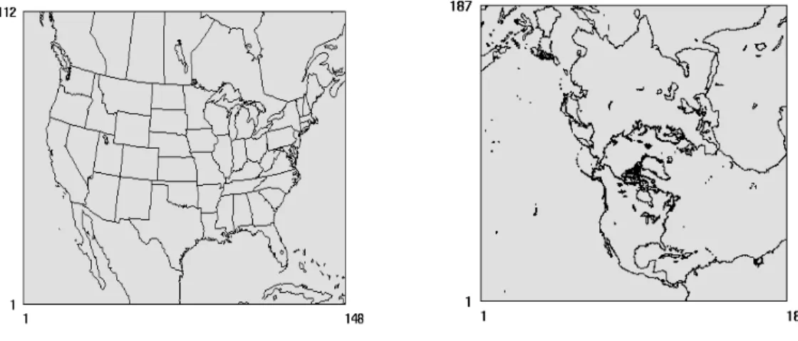
Figure 2.1: 36 × 36 km2 Continental US domain (left, with black square showing 7
the 4 × 4 km2 model domain) and 4 × 4 km2 northeast US (right) domain 8
with location of PVD airport (black aircraft icon). ... 12 9
10
Figure 2.2: Pie chart representing the percentage contribution from HAPs to 11
annual airport TOG emissions in the sensairp_4km case (left) and monthly 12
airport emissions in the airport grid-cell (right). ... 14 13
14
Figure 2.3: AQS monitoring sites (left, red pointers) with location of PVD airport 15
(red aircraft icon) and RIDEM monitoring sites (right, blue pointers) around 16
the airport (Courtesy: Google map). ... 17 17
18
Figure 2.4: Monthly average all source (sensairp_4km) (top) and airport- 19
attributable (sensairp_4km minus base_4km) (bottom) concentrations in the 20
PVD airport 4×4km grid-cell. ... 21 21
22
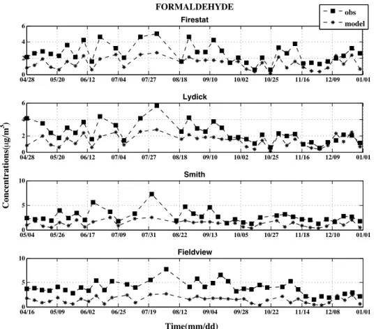
Figure 2.5: Time-series of modeled and observed formaldehyde daily average 23
concentrations at RIDEM sites. ... 22 24
25
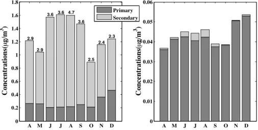
Figure 2.6: Secondary and Primary Formaldehyde monthly averaged 26
concentrations from all sources (left) and airport-attributable (right) in the 27
PVD airport grid-cell from April to December 2005. Also shown as labels 28
on each bar plot in the left figure are monthly averaged observational data 29
from three RIDEM sites (Fieldview, Lydick, Firestation) that fall in the 30
PVD 4 × 4 km2 grid cell. ... 23 31
32
Figure 2.7: Comparison between sensairp_36km and sensairp_4km model 33
scenarios normalized mean bias (%) at the Fieldview site. ... 26 34
35
Figure 2.8: Top panel shows bar plot of formaldehyde aircraft emissions 36
differences at the PVD airport grid-cell between sensairp_4km_4perc and 37
sensairp_4km simulations with their fractional increase value shown as label 38
on top of each bar. Bottom panel shows the primary (left) and secondary 39
formaldehyde (right) aircraft attributable increases in the 40
sensairp_4km_4perc simulation when compared with sensairp_4km. ... 27 41
42
Figure 2.9: Box plots comparison of CMAQ data with observation data for April– 43
December 2005 with an overlay of NATA census tract annual value (star 44
symbol) near one RIDEM (Smith) and one AQS (Providence) site. ... 31 45
Figure 3.1: Modeling domains (CONUS – left) and (HEMI – right). ... 40 1 2
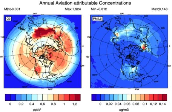
Figure 3.2: Aviation-attributable contributions of annual averaged O3 (left) and 3
PM2.5 (right) for the hemispheric domain (HEMI) at the surface. ... 47 4
5
Figure 3.3: Aviation-attributable contributions of annual averaged O3 (left) and 6
PM2.5 (right) at the surface for three sub-regions NA (top), EU (middle), and 7
EA (bottom). ... 48 8
9
Figure 3.4: Aviation-attributable contributions domain wide average of 8-hour 10
daily maximum O3 (red) and daily averaged PM2.5 (blue) in the HEMI 11
domain (left panel). The domain wide average of monthly averaged 12
speciated aerosol PM2.5 AAC in the HEMI domain at the surface (right 13
panel). ... 50 14
15
Figure 3.5: The aviation contribution percentage (ACP,%) to total annual average 16
O3 (left) and PM2.5 (right) when compared with all other emission sources in 17
the entire HEMI domain and for all three sub-regions of NA, EU and EA. 18
The vertical data is stratified into near boundary layer (BL), mid- 19
troposphere (MT) and upper troposphere (UT). ... 52 20
21
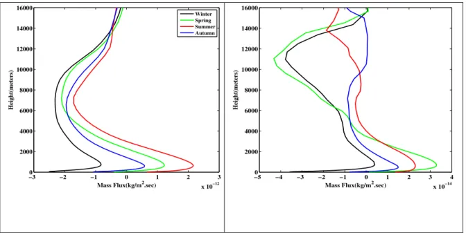
Figure 3.6: Vertical profile of O3 (left) and PM2.5 (right) aviation-attributable mass 22
flux (AMF) in the entire HEMI domain. Data is averaged over each season 23
in 2005 defined as: Winter = December – February, Spring = March – May, 24
Summer = June – August, and Autumn = September – November. ... 53 25
26
Figure 3.7: Vertical profile of O3 (left) and PM2.5 (right) aviation-attributable 27
mass flux (AMF) from NA (top), EU (middle) and EA (bottom) sub-regions 28
from HEMI domain. The data is seasonally averaged similar to description 29
mentioned in Figure 3.6. ... 54 30
31
Figure 3.8: Latitude cross-sectional plot of seasonal average O3 aviation- 32
attributable concentrations interpolated along isentropic levels for all four 33
seasons in HEMI domain. The left axis represents the isentropic levels, 34
right axis represents the average height for those isentropic model vertical 35
levels and bottom axis shows the latitudes in HEMI domain. The black 36
dashed overlay lines are the potential temperature (theta) in our modeling 37
domain. ... 57 38
39
Figure 3.9: Latitude cross-sectional plot of seasonal average PM2.5 aviation- 40
attributable concentrations interpolated along isentropic levels for all four 41
seasons in HEMI domain. The left axis represents the isentropic levels, 42
right axis represents the average height for those isentropic model vertical 43
levels and bottom axis shows the latitudes in HEMI domain. The black 44
dashed overlay lines are the potential temperature (theta) values in our 45
Figure 3.10: Comparison of modeled predictions of NO2 (top) and O3 (bottom) 1
from scenarios NoAirc36 (green), Airc36 (red), and Airc108 (blue) paired 2
with INTEX-NA observations (black) and binned vertically. Each point 3
represents the mean concentration value in a particular altitude bin of paired 4
modeled and observations. The bar plot (right) shows the number of paired 5
values in each bin. ... 62 6
7
Figure 3.11: Annual average aviation-attributable contributions of O3 (left) and 8
PM2.5 (right) for CONUS (36 km) domain. ... 64 9
10
Figure 4.1: Hemispheric modeling domain with cruise altitude emissions 11
distributions for complete northern hemisphere (top, left). Also shown are 12
the tagged cruise aviation emission scenarios for North America (top, right), 13
Europe (bottom, left) and East Asia (bottom, right). ... 76 14
15
Figure 4.2: Tracer surface mass fraction percentage with respect to the total mass 16
available in the each month. Each row is a single simulation where tracers 17
were reset to zero at the first month of each row and represents each season. ... 80 18
19
Figure 4.3: The amount of tracer (%) in each model vertical altitude (points on the 20
line) with respect to the total mass available in the model domain for each 21
month in a season. ... 82 22
23
Figure 4.4: Tracer mixing ratios for the last month in each 90 day simulation. 24
Each box plot represents the tracer mixing ratios for all horizontally grid 25
cells containing latitude bins of 0 – 30N (blue), 30 – 60N (green), and 60 – 26
90N(red). The tracer mixing ratios are further binned vertically by altitudes. ... 83 27
28
Figure 4.5: North America tracer surface mass fraction percentage with respect to 29
the total mass available in the model domain for each month. Each row is a 30
single simulation where tracers were reset to zero at the first month of each 31
row and then ran for 3 months in each season. ... 84 32
33
Figure 4.6: Europe tracer surface mass fraction percentage with respect to with 34
respect to the total mass available in the model domain for each month. 35
Each row is a single simulation where tracers were reset to zero at the first 36
month of each row and then ran for 3 months in each season. ... 86 37
38
Figure 4.7: East Asia tracer surface mass fraction percentage with respect to the 39
total mass available in the model domain for each month. Each row is a 40
single simulation where tracers were reset to zero at the first month of each 41
row and then ran for 3 months in each season. ... 87 42
43
Figure A1: Vertical profile of model layers height (left) and aircraft annual 44
emissions (right) for all HAPs. Note that aircraft emissions during LTO are 45
Figure A2: Bar plots comparing mean modeled values (all emissions sources) 1
with observation data at RIDEM (5 sites) and AQS (2 sites). ... 106 2
3
Figure A3: Bar plots comparing mean modeled values (all emissions sources) 4
with observation data at RIDEM (5 sites) and AQS (4 sites). ... 107 5
6
Figure A4a: Annual all source (sensairp_4km, left) and PVD airport-attributable 7
(sensairp_4km minus base_4km, right) concentrations of formaldehyde 8
(top), acetaldehyde (middle) and benzene (bottom). ... 108 9
10
Figure A4b: Annual all source (sensairp_4km, left) and airport-attributable 11
(sensairp_4km minus base_4km, right) concentrations of acrolein (top), 1,3- 12
butadiene (middle) and naphthalene (bottom). ... 109 13
14
Figure A4c: Annual all source (sensairp_4km, left) and airport-attributable 15
(sensairp_4km minus base_4km, right) concentrtions of xylene (top) and 16
toluene (bottom). ... 110 17
18
Figure A5: CMAQ 36 × 36 km2 model performance near NATTS sites (blue 19
dots) and 99 major airports (red aircraft), bar charts representing Normalized 20
Mean Bias (NMB, %) for sensairp_36km. ... 113 21
22
Figure A6: CMAQ 36 × 36 km2 model performance near NATTS sites (blue 23
dots) and 99 major airports (red aircraft), bar charts representing difference 24
between sensairp_36km and base_36km normalized mean error (NME, %). ... 114 25
26
Figure A7: NATA and CMAQ total (all sources, top) and airport concentrations 27
(bottom) in Kent county, Rhode Island (where PVD airport is located). ... 116 28
29
Figure B1: Monthly average aviation-attributable surface concentrations of O3 in 30
HEMI domain ... 123 31
32
Figure B2: Monthly average aviation-attributable surface concentrations of PM2.5 33
in HEMI domain ... 124 34
35
Figure B3: Daily domain-wide average AAC (left) of O3 (red), PM2.5 (blue) for 36
NA (top), EU (middle) and EA (bottom) sub-regions from HEMI domain at 37
the surface. ... 125 38
39
Figure B4: NME (%) spatial plots averaged over the year 2005 of hourly O3 (top) 40
and PM2.5 (bottom) predicted by Airc36 (CONUS, left panel) and Airc108 41
(HEMI-NA, right panel) model scenarios in comparison with hourly AQS 42
observations. ... 126 43
Figure B5: NMB (%) spatial plots averaged over the year 2005 of hourly O3 (top) 1
and PM2.5 (bottom) predicted by Airc36 (CONUS, left panel) and Airc108 2
(HEMI-NA, right panel) model scenarios in comparison with hourly AQS 3
observations. ... 127 4
5
Figure B6: Monthly soccer plots of O3 (top) and PM2.5 (bottom) for Airc36 6
(CONUS, left panel) and Airc108 (HEMI-NA, right panel) model scenarios 7
when compared with AQS observations. ... 128 8
9
Figure B7: Comparison of modeled predictions of HNO3 (top) and PAN (bottom) 10
from scenarios NoAirc36 (green), Airc36 (red), Airc108 (blue) paired with 11
INTEX-NA observations (black) and binned vertically. Each point 12
represents the mean concentration value in a particular altitude bin of paired 13
modeled and observations. The bar plot (right) shows the number of paired 14
values in each bin. ... 129 15
16
Figure B8: NMB (%) vertical profiles of hourly O3 predicted by the Airc108 17
model scenarios when compared with MOZAIC in-situ aircraft observation 18
data at four airports (Beijing, Munich, New Delhi, Shanghai). Also shown 19
are the NME differences between NoAirc108 and Airc108 scenarios. ... 130 20
21
Figure B9: NMB (%) vertical profiles of hourly O3 predicted by the Airc108 22
(black line) and Airc36 (red line) model scenarios when compared with 23
MOZAIC in-situ aircraft observation data from four NA airports (Atlanta, 24
Chicago, New York, San Francisco). ... 131 25
26
Figure B10: Monthly average aviation-attributable surface concentrations of O3 in 27
CONUS domain ... 132 28
29
Figure B11: Monthly average aviation-attributable surface concentrations of 30
PM2.5 in CONUS domain at the surface. ... 133 31
32
Figure B12: Daily domain-wide average AAC (left) of O3 (red), PM2.5 (blue) and 33
monthly domain-wide average speciated PM2.5 (right) AAC for CONUS 34
domain (36 km) at the surface. ... 134 35
36
Figure B13: Monthly average ACC spatial plots of a) HEMI-NA (top), b) HEMI- 37
NEI-NA (middle) and difference (b-a, bottom) in January (left) and July 38
(right) for O3. ... 135 39
40
Figure B14: Monthly average AAC spatial plots of a) HEMI-NA (top), b) HEMI- 41
NEI-NA (middle) and difference (b-a, bottom) in January (left) and July 42
(right) for PM2.5. ... 136 43
Figure B15: Comparison of monthly averages aviation-attributable PM2.5 1
concentrations from three cases a) HEMI-NA (108km) (left) b) HEMI-NEI- 2
NA (middle) c) CONUS (36km) (right) for January (top panel) and July 3
(bottom panel) months The color bar limits are similar between a) and b) 4
cases but for c) we used a lower limit to capture the spatial variation in 5
CONUS. ... 137 6
7
Figure B16: Comparison of monthly averages aviation-attributable O3 8
concentrations from three cases a) HEMI-NA (108km) (left) b) HEMI-NEI- 9
NA (middle) c) CONUS (right) (36km) for January (top panel) and July 10
(bottom panel) months. The color bar limits are similar between a) and b) 11
cases but for c) we used a lower limit to capture the spatial variation in 12
CONUS. ... 138 13
14
Figure B17: Mean (top) and Maximum (bottom) domain-wide daily aviation- 15
attributable O3 contributions for three cases (HEMI-NA, HEMI-NEI-NA, 16
CONUS) for January and July months. ... 139 17
18
Figure B18: Mean (top) and Maximum (bottom) domain-wide daily aviation- 19
attributable PM2.5 contributions for three cases (HEMI-NA, HEMI-NEI-NA, 20
CONUS) for January and July months. ... 140 21
CHAPTER 1: INTRODUCTION
The association of air pollution to adverse human health has been well established from
numerous studies ( Lim et al., 2012; Caiazzo et al., 2013; Holliday et al., 2014), and assessing air
quality impacts from various sources to develop policy action is needed to protect public health.
State-of-art atmospheric modeling evolved as one essential tool to study air quality impacts and
undertake measures to mitigate effects from various emission sources. It is also important to
improve the modeling applications and evaluate them to better predict emission sources impacts.
In recent years, transportation has become one of the major emission sectors contributing to
ambient air pollution and health impacts throughout the world.
Aviation is the one of fastest transportation modes whose growth increased tremendously
due to commercial travel, worldwide trade, and technology improvements in both developed and
developing countries. Steady growth of 5% in passenger and 6% in freight transportation per
year has been observed since 1950. It accounts for ~ 10% and 30% of passenger-km traveled and
goods traded internationally (Schäfer and Waitz, 2014) in recent years. In future years, the
average annual growth rate is predicted to increase around 4.6% per year from 2010 to 2030
(Federal Aviation Administration (FAA), 2010). Till last year, it was one of the single largest
green house gas (GHG) emitting transportation sectors that was not subjected to U.S
Environmental Protection Agency (EPA) GHG standards. This year both EPA (U.S EPA, 2016)
and ICAO (ICAO, 2016) announced a CO2 standard for new aircraft delivered after 2028;
2016) for commercial aircraft. These recent regulatory standard implementations show the
efforts undertaken by federal agencies to reduce the aircraft emissions impacts on air quality,
human health and climate change. Therefore the major focus in this thesis is the aviation sector
and to improve modeling of aviation emissions to better characterize their air quality impacts.
Wilkerson et al., (2010) indicated that in 2006, the commercial aircraft fleet flew 31.26
million flights covering 38.68 billion kilometers by burning 188.20 million metric tons of fuel,
which contributes to 3% of current global annual fossil fuel usage. The Organization of
Petroleum Exporting Countries (OPEC) (Mazraati, 2010) mentioned aviation as second major
consumer with 11.2% of total oil demand in transportation sector and projected that fuel
consumption will increase from 188 Tg in 2002 to 327 Tg in 2025 (Eyers et al., 2004). Efforts
are already underway to use bio-fuels and low emission fuels for automobiles; however,
application of these enhanced alternative fuels for aviation industry may present various
challenges. There are several ongoing research activities both within and outside the U.S to
address these issues. Measurement campaigns such as NASA’s Alternative Aviation Fuel
Experiment (AAFEX) showed reduction in particulate emissions (Beyersdorf et al., 2014), black
carbon (Speth et al., 2015) due to alternative jet fuels and other synthetic jet fuels. Health impact
assessments (Morita et al., 2014) concluded that alternative fuels and technology improvements
could reduce mortality rate by 72% and 59% respectively when compared with 2050 reference
scenario. In recent times, major technological modifications have been made to increase engine
efficiency and to reduce fuel consumption, although the projected growth and associated
environment impacts can offset those improvements (Masiol and Harrison, 2014). Particularly
implementation of these technologies in developing countries in near future will be a key
Asia flight departures (Wasiuk et al., 2016) between 2005 – 2011 and expected to see 10%
(Brunelle-Yeung et al., 2014) increase in growth particularly in countries like China and India.
Therefore, this growth in aviation activity can implicate aircraft emissions to cause significant air
quality, climate and health impacts in coming years worldwide. Aviation is also one of the
anthropogenic emissions sources that can affect environment at local scale (air quality near
airports, noise), regional scale (air pollution) and global scale (air pollution and climate change)
(Schäfer and Waitz, 2014) as shown in Figure 1.1. The areas highlighted in orange color
rectangle boxes are the ones related to air quality impacts, which are some of the key interests in
this dissertation.
Like any other combustion source, aircraft emits various pollutants including Nitrogen
oxides (NO + NO2 = NOx), Sulfur dioxides (SO2), Carbon Monoxide (CO), Volatile Organic
Compounds (VOC), Carbon dioxide (CO2), Fine Particulate Matter (PM2.5) (particulate matter of
size less than 2.5 microns) and other unburnt hydrocarbon related pollutants (Hazardous Air
Pollutants) during various stages of flight activity. These emissions are mainly categorized into
landing-takeoff (LTO) and cruise altitude aviation emissions (CAAE) based on the engine thrust
and flight path. The LTO is further divided into idling, taxing, approach and climb out stages.
Different stages of flight path emit different pollutants, for example during idling, unburnt
hydrocarbons and CO emissions are high, and during cruising stage NOx emissions are higher. Dessens et al., (2014) mentioned that on a global scale, aviation NOxemissions are about 10% of
on-road (50% of total traffic) and 20% of shipping NOx (30% of total traffic) emissions. In the U.S, aviation NOx is three percent of the total transportation NOx, but near some major airports like Atlanta (ATL) and New York (JFK) it can contribute ~3% and ~15% to area NOx and
4
undergo various atmospheric transport and chemical changes by interacting with background
emissions (from other non-aviation sources) locally near urban areas and in the upper
troposphere. These pollutants can even perturb the greenhouse gases such as methane (CH4) and
ozone (O3), thereby causing local-scale as well as global-scale air quality and climate impacts.
Figure 1.1: Aviation emissions and their environmental impacts (Source: Masiol and Harrison, 2014) and areas highlighted with orange boxes are some of the fields related to aviation air quality impacts.
Early measurement studies (Clark et al., 1983) observed violations of the health-based
standards for CO and hydrocarbons (HC), that contributed significantly to the existed
photochemical oxidant issues near the airport terminals and runways at some of the major
airports. Since then many LTO aviation emissions based modeling studies (Unal et al., 2005;
Arunachalam et al., 2011; Woody et al., 2011) and observational studies (Turgut and Rosen,
M
ANUS
C
R
IP
T
AC
C
EP
TE
D
ACCEPTED MANUSCRIPT
4127
Figure 2. Simplified diagram of a turbofan engine (upper left); products of ideal and actual 4128
combustion in an aircraft engine (upper right); and related atmospheric processes, products, 4129
environmental effects, human health effects and sinks of emitted compounds (bottom). Adapted 4130
from Prather et al. (1999), Wuebbles et al. (2007) and Lee et al. (2009). 4131
2010; Nikoleris et al., 2011; Zhu et al., 2011) focused on key pollutants (O3, PM2.5, NOx , VOC) and their contribution in the vicinity of airports. These studies improved our understanding of air
quality impacts from LTO aviation emissions and their sensitivities near urban and airport areas.
As stated in Ratliff et al., 2009, almost ~150 airports in U.S are located near urban areas that are
in non-attainment (i.e., areas that exceeded NAAQS (National Ambient Air Quality Standards))
for one or more criteria pollutants.
Based on model predicted LTO air quality impacts, Brunelle-Yeung et al., (2014) showed
~ 210 deaths per year in contiguous U.S with ~11 and 39 premature mortalities reductions due to
desulfurization and NOxstringency policy scenarios. Another future year US major airports (99
airports) risk analysis study (Levy et al., 2012) projected a factor of ~6 increase in 2025
mortality when compared to 2005 (~180 deaths per year) due to LTO emissions. Overall these
studies indicated consistent air quality (O3, PM2.5, NOx) and health impacts attributable to LTO
aviation emissions for key pollutants. There is, however, no study on model assessment of
Hazardous Air Pollutants (such as formaldehyde, acrolein and acetaldehyde) and their impacts
near airports using a chemistry transport model. Research performed by Airport Cooperative
Research Program (ACRP) ( Wood et al., 2008; Herndon et al., 2012) stated the research gaps
(such as emission inventories missing low thrust HAPs emissions, emissions dependency with
ambient conditions) and ongoing monitoring efforts to study HAPs near airports. These reports
also stressed the need for quantifying the aircraft impacts through HAPs modeling near airports.
One other known gap was lack of detailed HAPs emissions estimates for aircraft. Therefore,
EPA and FAA (FAA, 2009) recently developed an aircraft-specific speciation profile, which is
Similarly, there are large uncertainties associated with full-flight and CAAE emissions
modeled air quality assessments. Globally, CAAE emissions (particularly NOx) are ~60 – 70%
(Olsen et al., 2013) among the total full-flight emissions when compared to LTO emissions.
These CAAE are not traditionally incorporated in regional scale modeling for studying air
quality, but given the role of intercontinental transport, high convection and deep mixing in
transporting pollutants from upper troposphere to surface ( Wild and Akimoto, 2001; Parrish et
al., 2004; West et al., 2009; Parrish et al., 2010) and vice versa, it is imperative to consider even
upper troposphere emission sources in assessing surface air quality impacts of aviation emissions
in their entirety. Allen et al., (2012) stated that natural emissions of NOx from lightning can
significantly increase upper tropospheric (20 ppbV) and surface (1.5 – 4.5 ppbV) ozone.
Aviation is the only anthropogenic source that emits emissions directly into the upper
troposphere, yet knowledge gaps still exists in assessing the magnitudes of CAAE impacts on
surface air quality and their associated health impacts. Previous studies showed widely varying
full-flight attributable health impacts estimates, ranging from ~ 405 (Morita et al., 2014) to ~
12,600 (Barrett et al., 2010) premature mortality per year due to aviation-attributable particulate
matter. Most of these studies used coupled climate (Jacobson et al., 2011; Morita et al., 2014)
and chemistry transport (Barrett et al., 2010) global models with coarse resolutions (4o × 5o, 2o ×
2.5o) to arrive at their exposure estimates. This shows that high range of uncertainty is involved
with health assessments related to CAAE, that perhaps could be improved through fine scale
modeling for better characterization of air quality predictions as mentioned in Jacobson et al.,
(2011) and Yim et al., (2015). Despite these global models indicating higher mortality due to
CAAE, very limited studies (Whitt et al., 2011) have focused on assessing the role of dynamic
aviation air quality literature. Therefore in this study, for the first time, we have used fine scale
model resolutions (108 × 108 km2, 36 × 36 km2) to quantify contributions of full-flight emissions
on air quality at northern hemispheric and regional scales. We also studied the role of transport
processes on CAAE at hemispheric scale.
Overall goal of this thesis dissertation is to study the aviation-attributable perturbations that
impact air quality at local, regional and global scales. The central hypothesis of this dissertation
is that fine scale modeling provides better characterization (spatial heterogeneity and temporal
variability) of aviation emissions impacts on air quality and health. To test this hypothesis, we
conducted a model-based assessment of aviation emissions impacts using U.S EPA’s
Community Multi-scale Air Quality (CMAQ) (Byun and Schere, 2006) modeling framework at
multiple scales ranging from local (4 × 4 km2) to hemispheric (108 × 108 km2) scale. We used
these enhanced modeling applications to address the uncertainties present in three main study
areas: aviation-related HAPs, full-flight emissions impacts and transport of cruise altitude
emissions to the surface. Investigating these areas will enhance our scientific understanding in
modeling aircraft emissions for assessing their impacts on surface air quality, and likely provide
an enhanced scientific basis for improved policy-making. The main objectives of the three study
areas are:
1. Estimate impacts of risk prioritized aviation-related HAPs near mid-sized airport due to
LTO emissions and discuss the model’s ability to predict HAPs near an airport at
different model resolutions (4 × 4 km2, 36 × 36 km2). Improve the model performance by
modifying aircraft HAPs emissions during idling, and assess the aviation-attributable
2. Quantify the full-flight (CAAE + LTO emissions) impacts on surface air quality and on
overall troposphere at hemispheric scale using the CMAQ model. Compare coarse and
fine resolution North America predictions and quantify the changes occurring in
aviation-attribution perturbations due to grid resolution (Chapter 3).
3. Assess the transport of cruise altitude emissions to surface at hemispheric scale by using
passive tracer based modeling. Additionally, tag the CAAE tracers in individual
sub-regions to study the intercontinental transport of aviation emissions and develop
source-receptor relationships (Chapter 4).
Finally in Chapter 5, the final conclusions from all three studies were discussed along with
the limitations. The future work to further improve the understanding of aviation-related air
CHAPTER 2: EVALUATION OF MODEL-PREDICTED HAZARDOUS AIR POLLUTANTS NEAR A MID-SIZED U.S. AIRPORT1
2.1 Introduction
Aviation has experienced proliferative growth in the past few decades. Commercial
aviation operations are rapidly increasing worldwide, with a growth rate of 61, 40, and 22
percent in large, medium, and small hub airports (FAA, 2011). The average annual growth rate is
predicted to increase around 4.6 percent from 2010 to 2030 (FAA, 2010). These quantitative
projections clearly indicate substantial aviation growth in future. This growth implicates
potential increase in aircraft emitted pollutants such as Nitrogen oxides (NOx), Sulfur oxides
(SOx), Particulate matter (PM), and Volatile Organic Compounds (VOC) including Hazardous
Air Pollutants (HAPs). Thus, there is a need to characterize impact of aviation emissions on local
air quality particularly in the vicinity of an airport as a first step to assess their impacts on the
environment and human health. Further, stringent emission standards on road transport (US
EPA, 2014) will likely increase the relative contributions from aviation emissions that impact
local air quality.
Although significant research has been undertaken quantifying the impact of PM2.5, NOx
and O3 near airports, there has been little focus on exposure assessment for HAPs.
Airport-related air-quality studies have focused mainly on NOx (Wood et al., 2008; Timko et al., 2010),
PM2.5 (Mazaheri et al., 2009) and CO due to their relatively higher contribution to the overall
1This chapter previously appeared as an article in Atmospheric Environment. The original
citation is as follows: Vennam, L. P., Vizuete, W., & Arunachalam, S. (2015). Evaluation of model-predicted hazardous air pollutants (HAPs) near a mid-sized US airport. Atmospheric
airport-related emissions (Schürmann et al., 2007). These studies measured emissions during
landing and takeoff conditions (LTO) and showed that these pollutants have significant impact
on air quality near the airport. Air-quality modeling studies have reported maximum impacts of
O3 and PM2.5 of 56 ppbV and 25 µg/m3 near Hartsfield-Jackson airport in Atlanta (Unal et al.,
2005). Arunachalam et al., (2011) showed that the LTO emissions could have 28-35% of impacts
in PM2.5 occurring 300km away from the airport due to secondary formation. Woody et al.,
(2011) reported that the other background emissions (from non-aviation sources) can have an
important role on the aviation-attributable impacts and the PM2.5 impacts in the airport grid-cell
is approximately twice the national average. These studies show that airport emissions have a
significant impact on air quality near airports and suggest that there could be significant
exposures of other emitted pollutants like HAPs.
HAPs are a listing of 187 pollutants that are known or suspected to cause serious health
effects specifically categorized in the 1990 Clean Air Act (CAA, Section 112). Recent studies
(Laurent and Hauschild, 2014) suggested that carcinogenic pollutants like HAPs have not been
controlled sufficient enough to protect public health. They reported that some of the key HAPs
such as formaldehyde and acrolein contributed only 6% and 0.2% of total NMVOCs
(non-methane volatile organic compounds), but account for 90% cancer effects and 89% non-cancer
effects respectively. The higher health risk pertaining to HAPs and their chemically reactive
nature in the atmosphere calls for more attention in local scale air-quality studies. Prior aviation
studies (Herndon et al., 2012) indicated that 15 of the 187 identified HAPs are observed in
aircraft exhaust. An aircraft-attributable health study (Levy et al., 2008) found that significant
local health effects such as cancer and cardiopulmonary risks were caused from air toxics in spite
HAPs as lower in priority compared to both PM2.5 and O3 due to aircraft emissions. Studies have
found that when compared to LTO operations there were 80 – 90% higher emissions during
idling-taxing, emitting several HAPs including: formaldehyde, acetaldehyde, benzene, ethylene,
propene and butenes + acrolein (Anderson et al., 2006; Herndon et al., 2006). Spicer et al.,
(1996) also reported that these seven pollutants make up ~75% of the volatile organic compound
(VOC) emissions that are being detected in aircraft exhaust. According to the Airport System
Performance Metrics database (ASPM, FAA), the average taxi time at mid-sized to large-sized
airports is reported in the range of 10 – 20 minutes, which is significant amount of time to emit
HAPs.
Though idle and taxi activities have the potential to impact air quality near airports,
limited studies exist with detailed model-based characterization of HAP emissions. With such
limited knowledge of aviation HAPs airport authorities are unable to provide effective guidance
to state and local constituencies. One known gap is the lack of detailed HAPs emissions
estimates from aircraft during LTO operations. In this study we have attempted to reduce these
uncertainties by using new FAA-EPA generated aircraft-specific speciation profiles (FAA, 2009)
for Total Organic Gases (TOGs) that estimate individual HAPs and differentiating emissions by
aircraft operating modes. To evaluate this model and current HAP modeling approaches we took
advantage of field observational data available at the T.F. Green airport (PVD) in Providence,
Rhode Island. The detailed modeling and evaluation performed in this study provides an
assessment of the tools that help airport regulatory authorities in making any decisions and
regulators to evaluate air quality and potential health risk associated with the HAPs in the
2.2 Methodology
We focused on eight major aviation health-risk prioritized (Levy et al., 2008) HAPs:
formaldehyde, acetaldehyde, acrolein, 1,3-butadiene, benzene, toluene, xylene and naphthalene.
Based on their toxicity levels, (Wood et al., 2008) also ranked these HAPs as important
near-airport exposure pollutants.
2.2.1 Air Quality Model (CMAQ)
We used the Community Multi-scale Air-Quality (CMAQ) (Byun and Schere, 2006)
model to evaluate the changes in HAPs emissions, as well as their impacts on ambient air
quality. Table 2.1 shows the model scenarios description and domain specifications considered in
this study. Figure 2.1 shows both 36 × 36 km2 and 4 × 4 km2 horizontal resolution model
domains whose model results for year 2005 were used for this evaluation.
Figure 2.1: 36 × 36 km2Continental US domain (left, with black square showing the 4 × 4 km2 model domain) and 4 × 4 km2 northeast US (right) domain with location of PVD airport (black aircraft icon).
The CMAQ 4 × 4 km2 scale resolution simulations were conducted in the Northeast U.S. for 2005 annual year with 100 x 100 horizontal grid cells as shown in Figure 2.1 (black square,
left side). Emissions from all sources go up to 22 vertical layers (~ 680 hPa) and aircraft
lowest ~1000 meters (3000 ft). The T.F. Green airport (PVD) in Providence, Rhode Island is
labeled in Figure 2.1 with an aircraft icon. CMAQ v5.0.2 model with revised Carbon Bond
(CB05) multi-pollutant mechanism (Yarwood et al., 2005; Whitten et al., 2010; CMAS, 2014)
and explicit air toxics chemistry (CB05TUMP_AE6_AQ) was used for the model simulations.
The meteorology input data (34 layers, ~130 hPa, Figure A1) were generated using the
Mesoscale Meteorological (MM5 v3.7.2) model (Grell et al., 1994). We used 2005 National
Emissions Inventory (NEI) (U.S EPA, 2007) to generate emissions for non-aviation sources,
which were processed using Sparse Matrix Operator Kernel Emissions (SMOKE) model
(Houyoux et al., 2000) to generate grid-based emissions that are speciated and temporally
allocated. The initial and boundary conditions are nested from 12 × 12 km2 CMAQ simulations
for the Eastern U.S.
Table 2.1: Specifications and description of modeling scenarios in the study
a) CONUS: Continental United States, b) NEI: National Emissions Inventory, c) EDMS: Emissions Dispersion Modeling System, d) AEDT: Aviation Environmental Design tool e) PVD: T.F.Green airport, RI
In this study, the aviation emissions were based on FAA’s Aviation Environmental
Design Tool (AEDT) (Wilkerson et al., 2010) segment data. This tool predicts emissions and Scenario
name
Period Grid Cell Resolution
Domain CMAQ version
Background emissions
Aviation emissions
Base_36km 01/01/05 -12/31/05
36 × 36 km2 CONUSa 4.6 NEIb-2005 No Sensairp_36k
m
01/01/05 -12/31/05
36 × 36 km2 CONUS 4.6 NEI-2005 EDMSc emissions (99 major airports) Base_4km 01/01/05
-12/31/05
4 × 4 km2 Northeast US
5.0.1 NEI-2005 No
Sensairp_4k m
01/01/05 -12/31/05
4 × 4 km2 Northeast US
5.0.1 NEI-2005 AEDTd emissions for PVDe airport
Sensairp_4k m_4perc
07/01/05- 08/31/05
&
11/01/05-12/31/05
4 × 4 km2 Northeast US
5.0.1 NEI-2005 AEDT emissions for PVD airport with modified 4% thrust
aircraft fuel use for all global commercial flights. From this highly resolved emissions inventory,
we selected flights arriving and departing from the PVD airport and processed them through
AEDTProc (Baek et al., 2012) . AEDTProc is a processing tool that takes chorded segments of
individual flight emissions and then creates CMAQ model-ready emissions inputs that were then
merged with the other non-aircraft emissions inventories. Speciated HAPs emissions were
estimated in AEDTProc using Total Organic Gases (TOG) speciation profile (FAA, 2009). This
speciation profile (Table A1) for aircraft engines was established by FAA and U.S. EPA based
on APEX (FAA, 2009) and EXCAVATE (Anderson et al., 2006) airport measurement
campaigns.
Figure 2.2: Pie chart representing the percentage contribution from HAPs to annual airport TOG emissions in the sensairp_4km case (left) and monthly airport emissions in the airport grid-cell (right).
For annual 2005, a total of 6.12 short tons of key HAPs were emitted by aircraft
representing 10% of total anthropogenic sources HAPs in the PVD grid cell. The pie chart in
Figure 2.2 (left) illustrates the composition of those emissions. NON-HAP TOG, defined as
VOCs other than HAPs is the largest contributor to TOG, and is further speciated into lumped
chemical species based upon the CB05 chemical mechanism. Formaldehyde, acetaldehyde, and 14.2%& 4.4%&
2.4%& 1.7%& 1.7%& 0.2%& 0.4%& 0.5%& 74.4%&
Formaldehyde& Acetaldehyde& Acrolein& Benzene& 1,3=Butadiene& Toluene& Xylene& Naphthalene& Non=HAP&TOG&
Jan Feb Mar Apr May Jun Jul Aug Sep Oct Nov Dec 0
0.1 0.2 0.3 0.4 0.5 0.6 0.7
Emissions(tons/month)
Monthly sum airport emissions
acrolein are key contributors (14.2%, 4.4%, 2.4%) to the annual aircraft HAPs emissions. Note
that AEDT does not include emissions from ground supporting equipment (GSE), ground
auxiliary vehicles (GAV) and stationary sources (Supp. Material Section2, Table A5). Figure 2.2
(right) shows the monthly total aircraft emissions of HAPs and shows the lack of any seasonal
trend i.e., higher emissions during lower temperatures (during winter months, emission index is
~3.5 times higher at 0° C compared to 25° C) as mentioned in observation based studies (i.e., no
(Herndon et al., 2012) temperature dependency in the emission inventory).
Finally we merged non-aviation emissions (background sources) with aviation emissions
to generate emissions input for Sensairp_4km case. Two annual model simulation scenarios
named, Base_4km and Sensairp_4km, are shown in Table 2.1. The difference in output between
these two cases accounts for the incremental aviation emissions contribution to ambient air
quality.
For this study we also completed an alternate emissions scenario (Sensairp_4km_4perc in
Table 2.1) to assess sensitivity due to increased taxi/idle condition hydrocarbon emissions based
on the findings from previous aircraft measurement studies ( Herndon et al., 2006; Beyersdorf et
al., 2012) . These observational studies indicated that the observed hydrocarbon emissions
indices (g/kg) are a factor of ~1.5–2.2 times greater than the International Civil Aviation
Organization (ICAO) specified certification benchmarks that are typically used to construct
aircraft emissions inventories. Therefore, we considered the latest 2005 AEDT emissions, and
modified the idle hydrocarbon emissions near PVD airport using the idling time spent by each
flight and extrapolated 4% emission index (HC_EI_4perc) from the ICAO database for different
doubling of aircraft LTO emissions at PVD when compared with sensairp_4km. However,
compositional profile of emitted HAPs and the lack of seasonal pattern remained the same.
As shown in Table 2.1, we performed this sensitivity model simulation for 4 months
(July–August (summer), November–December (winter)) to create the Sensairp_4km_4perc
(background + 4% thrust airport emissions) case. Therefore, the difference between
Sensairp_4km_4perc and Base_4km cases gives us the incremental aviation contributions with
the improved idle emissions.
2.2.2 Observational Data
Availability of near-airport field-based measurements of HAPs at PVD provided us the
opportunity for detailed model evaluations. These included measurements of HAPs completed by
the Rhode Island Department of Environmental Management (RIDEM) in and around the PVD
airport. In the RIDEM study campaign, sampling was conducted at five monitor sites near the
airport for the period April 2005 to August 2006. Four of these sites (Fieldview, Firestation,
Lydick, Smith) are located near the airport and one site (Draper) is located 2.3 miles from the
main runway (RIDEM, 2008). The Fieldview site is ideally located near the main runway where
86% of airplane activity at PVD occurs (Dodson et al., 2009). All three sites Fieldview,
Firestation and Lydick fall in the PVD airport 4 × 4 km2 grid-cell in our modeling domain. Along with the five RIDEM sites near the airport, we used four additional sites from EPA’s Air Quality
System (AQS) to understand the relative difference in airport-attributable concentrations
between urban, rural and airport sites. Figure 2.3 shows the spatial location of AQS sites (red
Figure 2.3: AQS monitoring sites (left, red pointers) with location of PVD airport (red aircraft icon) and RIDEM monitoring sites (right, blue pointers) around the airport (Courtesy: Google map).
We also compared model predictions against observations from the National Air Toxics
Trends Stations (NATTS, (US EPA, 2009)) (Supp. Material Section A3.2). Figure A5 shows the
U.S. map with red aircraft symbols indicating the 99 airports and blue pointers indicating the
collocated NATTS sites near the airports for year 2005. Table A4 shows the location of NATTS
sites and major airports in CMAQ model grid cells.
2.2.3 HAPs estimates from NATA
CMAQ predicted annual average concentrations were compared with annual estimates
from the National Air Toxics Assessment (NATA) (US EPA, 2011). NATA is a
state-of-the-science screening tool developed by U.S. EPA in collaboration with state and local agencies, to
evaluate the health risks involved with air toxics both at regional and local level. NATA outputs
are at census-block resolution for the entire nation. For these estimates, NATA used a
combination of predictions from the AERMOD dispersion model for primary and CMAQ (using
12×12 km2 resolution) for the secondary contribution of formaldehyde, acetaldehyde, and
acrolein. The recent 2005 NATA annual modeling data were obtained from updated emissions
inventory that considered airport emissions from 20,000 U.S. airports (US EPA, 2011).
Pawtucket)
Providence)
E.Providence)
W.Greenwich)
!" !"#$%&'()*+,")-%./01%23%456%7-8%!9:;"8%
/)8'*"-#%<);%=;)>"8'-?'%0";@);,
A">'%&BCD/%EFFG%5'7(+;'5'-,%(",'(%7;'%($)H-0-%'I';?"('%)<%5)8'*J87,7%?)5@7;7,">'%7-7*9("(
!"#$ %&'&"()
%*"&+ !"$,-."$/
01-"2
2.3 Results
In this section, we organize our results into 3 major sub-sections – model evaluation
against observations, comparison of model predictions from two different resolutions, and finally
comparison against another published source. First we show the model evaluation for 4 × 4 km2
applications against 4 × 4 km2 observational data and discuss the trends in aircraft contributions in the airport grid-cell. We then compare 4 × 4 km2 model performance with 36 × 36 km2 and discuss differences observed between the two resolutions. Later we present the aircraft emission
sensitivity results and the increase in aircraft-attributable concentrations due to the modified idle
aircraft emissions. Finally we compare our CMAQ model results with those from EPA’s NATA
to understand the differences between these two model predictions.
2.3.1 Model Evaluation: 4 × 4 km2grid resolution
The sensairp_4km simulation’s ability to predict concentrations accurately varies by
pollutant and spatial location as shown by the overall Normalized Mean Error (NME) and
Normalized Mean Bias (NMB) in Table 2.2. From Table 2.2 (top panel), the NME averaged for
all sites is between 36–70% for all pollutants except for acrolein (NME: ~90%). Acrolein shows
the largest NME of ~90% regardless of site location. This high underprediction of acrolein has
been observed in prior studies. For example, (Luecken et al., 2006) pointed the uncertainties in
emissions and highly challenging acrolein sampling (Seaman et al., 2009) as a source of
observational difficulty. A recent study (Cahill, 2014) also measured acrolein background
concentrations that were higher than the EPA’s reference concentrations (for health risk), but due
to sparse data they were unable to come to a definite conclusion on acrolein exceedances and
Table 2.2 shows that NME was higher for the AQS sites when compared to RIDEM sites;
36% higher for xylene and 23% higher for toluene. Consistent with the NME results the model
overpredicted (NMB: 24–41%) concentrations of xylene, toluene and benzene at all sites with
the W. Greenwich and E. Providence AQS sites (Figure A3) showing the largest overpredictions.
These errors for xylene and toluene are mainly driven by the W. Greenwich AQS site (Figure
2.3) at a rural location 33 km from the airport. This AQS site had a NME of 100-200%
consistently throughout the year for xylene and toluene.
The RIDEM sites had a higher NME for formaldehyde (11%) and 1,3-butadiene (7%)
when compared to the AQS sites. As shown in Table 2.2 (bottom panel) the formaldehyde NMB
is -52% at RIDEM sites and -31% at AQS sites. The largest underprediction of formaldehyde
was at the Fieldview RIDEM site with a NMB of -60%. Spatially (Figure A2), observations
show ~1.5 times higher concentrations near Fieldview (3.93 µg/m3) when compared to all other
sites. The model-predicted period average of 1.44 µg/m3 was far below the observed high
concentrations at the Fieldview site.
To understand the contribution that the new highly resolved aircraft emissions had on
HAP model performance we re-ran the simulation without aircraft emissions (base_4km). The
NME and NMB values from base_4km are shown in Table 2.2 inside parenthesis. From Table
2.2 it is clear that aircraft emissions had an impact of less than 0.1% on model error at the AQS
sites. The largest changes in model prediction from aircraft emissions occurred at the RIDEM
sites where additional aircraft emissions improved the NME for formaldehyde (1%) and xylene
(2.3%). It is clear from NMB that additional formaldehyde emissions reduced the
underprediction by 1.1%. The increased aviation emissions had the largest impact on NMB and
aircraft emissions did increase the NME in the case of 1,3-butadiene (4.6%), benzene (0.4%) and
toluene (0.1%). The model was already overpredicting these species, so the addition of aircraft
emissions caused the model to increase overprediction for these species.
Table 2.2: Annual NME (%, top) and NMB (%, bottom) using pollutant predictions from the sensairp_4km averaged for all sites and differentiating RIDEM and AQS sites. Also shown in parenthesis are the base_4km case (with no airport emissions) values.
Pollutant All sites RIDEM AQS
NME NME NME
Acrolein 91.6 (91.6) 92.4 (92.4) 92 (92) Formaldehyde 49.1 (49.8) 52.4 (53.3) 41 (40.9)
Acetaldehyde 33.6 (33.6) 33.1 (33.1) 34.8 (34.8) 1,3-Butadiene 57.6 (57.5) 60.5 (57.9) 53.9 (53.8) Xylene 69.1 (70.5) 55.3 (55.3) 89.6 (89.6) Benzene 58 (57.5) 58.5 (58.1) 57.2 (57.1) Toluene 71.7 (71.6) 61.7 (61.6) 84.2 (84.2)
Pollutant All sites RIDEM AQS
NMB NMB NMB
Acrolein -91.6 (-91.6) -92.4 (-92.4) -91.7 (-91.7) Formaldehyde -45.6 (-46.4) -51.5(-52.6) -31.0(-31.0) Acetaldehyde -7.1 (-7.6) 1.1 (0.3) -27.6(-27.6) 1,3-Butadiene -2.3(-5.6) 9.0(3.1) -16.4(-16.6) Xylene 24.4(28.7) 17.6(17.4) 42.8(42.8) Benzene 30.2(29.8) 31.9(31.2) 28.1(28) Toluene 41.2(41.1) 28.5(28.4) 57.0(57.0)
From the model performance data it is clear that aviation emissions only impacted HAP
concentrations at monitors that were within 1–2 km from the airport. Thus, our analysis focused
on the contributions of HAPs from the newly added emissions in just the PVD airport grid-cell
(which contains RIDEM monitors Fieldview, Lydick and Fire Station). In supplementary
contributions of the aircraft-attributable for January and July months, which are in the range of
0.5–28% in the airport grid-cell. Figure 2.4 shows the monthly averaged increases in
concentrations of airport-related HAPs (sensairp_4km minus base_4km, bottom) and total
concentrations from all sources (sensairp_4km, top) in the airport grid-cell. Though aviation
emissions of HAPs were relatively constant throughout the year, the contributions of HAPs
concentrations were higher during winter months than summer months due to their shorter
lifetime in the atmosphere during summer than winter.
Figure 2.4: Monthly average all source (sensairp_4km) (top) and airport-attributable
(sensairp_4km minus base_4km) (bottom) concentrations in the PVD airport 4×4km grid-cell.
Figure 2.5 shows the time series of observed and modeled (sensairp_4km) formaldehyde
concentrations near RIDEM sites (not included Draper due to fewer hours of observation
Jan Feb Mar Apr May Jun Jul Aug Sep Oct Nov Dec
0 5 10 15
Concentrations(
µ
g/m
3 )
Jan Feb Mar Apr May Jun Jul Aug Sep Oct Nov Dec
0 0.05 0.1 0.15
Concentrations(
µ
g/m
3 )
Formaldehyde Acetaldehyde Acrolein 1,3−Butadiene
available) for the RIDEM study campaign period. The model was able to capture the temporal
variability near all sites, although it is clear that the concentrations are underpredicted. The
underprediction is high mainly near Fieldview runway site where the highest formaldehyde
concentrations were predicted. The model was also unable to predict the largest observed peaks
during the summer months.
Figure 2.5: Time-series of modeled and observed formaldehyde daily average concentrations at RIDEM sites.
To understand the primary (directly emitted) and secondary (formed due to atmospheric
chemistry) contribution to total formaldehyde in the airport grid-cell we looked at these
concentrations separately. In this simulation of CMAQ, the formaldehyde emissions were
reported explicitly as primary formaldehyde (FORM_PRIM) and tracked separately from total
FORMALDEHYDE
Concentrations(
µ
g/m
3 )
Time(mm/dd)
04/160 05/09 06/02 06/25 07/19 08/12 09/04 09/28 10/22 11/14 12/08 01/01 5
10 Fieldview
05/040 05/26 06/17 07/09 07/31 08/22 09/13 10/05 10/27 11/18 12/10 01/01 5
10 Smith
04/280 05/20 06/12 07/04 07/27 08/18 09/10 10/02 10/25 11/16 12/09 01/01 2
4
6 Lydick
04/280 05/20 06/12 07/04 07/27 08/18 09/10 10/02 10/25 11/16 12/09 01/01 2
4
6 Firestat