INVESTIGATION OF THE 30Si(p,γ)31P REACTION
John Robert Dermigny
A dissertation submitted to the faculty at the University of North Carolina at Chapel Hill in partial fulfillment of the requirements for the degree of Doctor of Philosophy in the Department
of Physics.
Chapel Hill 2018
c 2018
ABSTRACT
John Robert Dermigny: Investigation of the 30Si(p,γ)31P Reaction
(Under the direction of Christian Iliadis)
Abundance anomalies in globular clusters provide strong evidence for multiple stellar popula-tions within each cluster. These populapopula-tions are usually interpreted as distinct generapopula-tions, with the currently observed second-generation stars having formed in part from the ejecta of massive, first generation “polluter” stars, giving rise to the anomalous abundance patterns. The precise nature of the polluters and their enrichment mechanism are still unclear. Even so, the chemical abundances measured in second-generation stars within the cluster NGC 2419 have provided insight into this puzzling process.
We performed a sensitivity study using Monte Carlo reaction rate network calculations based on a simple enrichment model for NGC 2419. This work suggested four thermonuclear reactions that have a significant impact on the elemental abundances in this cluster. A firm understanding of the astrophysical source of the pollution material is precluded by their large reaction rate uncertainties. In the present study, one of these reactions,30Si(p,γ)31P, has been investigated at the Laboratory
for Experimental Nuclear Astrophysics (LENA). The resonance strengths of theElab
r = 433.5±0.3
keV and Elab
r = 499.5 ±0.2 keV resonances have been measured. For the former, which was
“So long, and thanks for all the fish.”
ACKNOWLEDGEMENTS
First, I would like to thank my wife, Alexandra, who has been an incredible source of inspiration for me these past couple months. She is the most hardworking and tenacious person I know, and I aspire to be more like her. She has borne the brunt of the tremendous commitment this document represents, taking on the full suite of responsibilities at home while I was writing in various cafes and libraries. It could not have been done without her steadfast support.
I am incredibly thankful for my parents, Jack and Susanne. They grew up with considerably less than I did, and made me and my siblings’ education a top-priority while accomplishing a great deal themselves. They encouraged hard work and curiosity and made sure that I had every opportunity to explore, experiment, and wonder. This dissertation is a testament to the sacrifices they made for their children.
My advisor, Christian Iliadis, has been an superb mentor. He is peerless in his dedication to his students and their professional development. I have benefited enormously from his careful eye for scientific writing and presentation, and am very grateful for all the time he spent working with me on my research papers and talks. I will fondly remember our espresso fueled discussions, trying to wrangle truth from some subtle piece of statistical sorcery.
I consider myself very lucky to have worked with Art Champagne. This thesis project most certainly would have been delayed if not for his support. When faced with the choice to either order my targets from a collaborator or refurbish and install the SNICS source, Art fully supported the latter. This was in spite of the potential risks involved with having a graduate student dismantling the work-horse ion source of TUNL. Getting the SNICS working would end up being one my prouder moments as a student.
experiments, analysis techniques, and other ideas by him. His careful approach to experimental physics and statistics has certainly left an indelible mark on me.
TABLE OF CONTENTS
LIST OF TABLES . . . xii
LIST OF FIGURES . . . xiii
1 Introduction . . . 1
1.1 Globular Clusters . . . 1
1.2 Abundance Anomalies . . . 4
1.3 NGC 2419 . . . 7
2 Nucleosynthesis Simulations . . . 10
2.1 Previous Work . . . 10
2.2 Sensitivity Study . . . 12
2.3 30Si(p,γ)31P . . . 15
3 Nuclear Astrophysics Theory. . . 17
3.1 Thermonuclear Reaction Rates . . . 17
3.2 Non-Resonant Reaction Rates . . . 18
3.3 Resonant Reaction Rates . . . 20
3.4 Gamow Peak . . . 22
4 Accelerators and Detector System . . . 24
4.1 LENA I, the JN Van de Graff . . . 25
4.3 The γγ-Coincidence Spectrometer . . . 29
4.3.1 Detection Efficiencies . . . 30
5 Fitting Method. . . 37
5.1 Introduction . . . 37
5.2 Analysis Method . . . 38
5.3 Geant4 Simulations . . . 41
5.3.1 General Strategy . . . 41
5.3.2 Corrections to Simulated Templates . . . 42
5.3.3 Background Contaminants . . . 44
5.4 Goodness of Fit Testing . . . 44
5.4.1 Run Test . . . 48
5.5 Summary . . . 51
6 Targets . . . 52
6.1 Silicon Targets . . . 52
6.1.1 Tantalum Backings . . . 53
6.1.2 SNICS Source . . . 54
6.1.3 Implantation . . . 57
6.1.4 Target Cleaning . . . 58
6.2 Target Yield Curves . . . 59
7 30Si(p,γ)31P Proton Capture . . . . 64
7.1 620 keV Resonance . . . 65
7.1.1 Measurement . . . 68
7.1.3 Resonance Energy . . . 74
7.2 498 keV Resonance . . . 75
7.2.1 Measurement . . . 76
7.2.2 Analysis . . . 78
7.2.3 Resonance Energy . . . 87
7.2.4 Resonance Strength . . . 88
7.3 435-keV Resonance . . . 89
7.3.1 Measurement . . . 91
7.3.2 Resonance Energy . . . 93
7.3.3 Analysis . . . 94
7.3.4 Angular Correlation Correction . . . 96
7.3.5 Resonance Strength . . . 102
8 Reaction Rate Evaluation . . . .105
8.1 Resonances . . . 105
8.1.1 Elab r >600 keV . . . 105
8.1.2 Elab r <600 keV . . . 107
8.2 Direct Capture . . . 113
8.3 Monte Carlo Reaction Rate Calculation . . . 115
9 CONCLUSION . . . .126
Appendix A Codes, Procedures, and Miscellanea . . . .128
A.1 Yield Curve Fitting . . . 128
A.2 Sum Correction Code . . . 132
A.4 Fraction Fitting Posterior Distributions . . . 137
Appendix B Calculations . . . .138
B.1 Detector Response . . . 138
B.2 Target Properties . . . 141
B.3 Bound State Branching Ratios . . . 143
Appendix C Bayesian Estimation. . . .144
LIST OF TABLES
6.1 Yield Curve Parameters . . . 62
7.1 Resonance Strength for 620 keV . . . 67
7.2 620 keV Intensities . . . 69
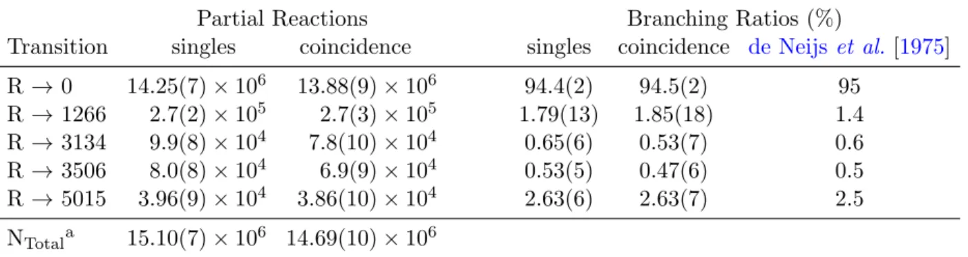
7.3 Partial Reactions for the 620-keV Resonance . . . 74
7.4 Resonance Strength for Elab r = 498 keV . . . 76
7.5 Yield Curve Parameters . . . 77
7.6 498 keV Intensities . . . 78
7.7 Angular Correlation Coefficients . . . 81
7.8 Partial Reactions for the 498-keV Resonance . . . 87
7.9 435 keV Intensities . . . 93
7.11 Angular Correlation Coefficients and Multipolarities . . . 100
8.1 Adopted Resonance Strengths . . . 108
8.2 Resonance Data . . . 113
8.3 Direct Capture S-Factor . . . 115
8.4 Tabulated Reaction Rate Parameters . . . 119
B.1 Geant4 Calculations for theγγ-coincidence spectrometer . . . 140
B.2 Calculated Stopping Powers . . . 142
LIST OF FIGURES
1.1 Color-Magnitude Diagram . . . 2
1.2 Triple Main Sequence . . . 5
1.3 Elemental Abundances of NGC 2419 . . . 8
2.1 The Temperature and Density Solutions for NGC 2419 . . . 12
2.2 Reaction Rate Sensitivity Results . . . 14
2.3 Nuclear Reaction Network for the Aluminum-Phosphorus Isotopes . . . 15
3.1 Experimental Cross Section and S-Factor . . . 19
3.2 Gamow Peak . . . 23
4.1 The Laboratory for Experimental Nuclear Astrophysics . . . 25
4.2 Dipole Magnet Calibration . . . 27
4.4 The LENAγγ-coincidence spectrometer . . . 30
4.5 Coincidence spectroscopy . . . 31
4.6 Measured Peak Efficiencies . . . 35
5.2 An Example of Overdispersion . . . 45
5.3 The Log-Likelihood Method . . . 47
5.4 The Run Test . . . 49
6.1 The Lena Evaporator . . . 53
6.2 SNICS Source Schematic . . . 55
6.3 SNICS Cage . . . 56
6.4 Implantation Beamline . . . 57
6.5 The SMIF Plasma Asher . . . 59
6.6 Yield Curve Comparison . . . 61
7.1 Energy level diagram for31P. . . 66
7.2 Pulse Height Spectrum taken at the Elab r = 620 keV resonance . . . 70
7.4 Posterior Plots - 620 keV coincidence . . . 73
7.6 Pulse Height Spectrum taken at the Elab r = 498 keV resonance . . . 79
7.7 Posterior Plots - 498 keV singles, I . . . 82
7.8 Posterior Plots - 498 keV singles, II . . . 83
7.9 Posterior Plots - 498 keV concidence, I . . . 84
7.10 Posterior Plots - 498 keV concidence, II . . . 85
7.12 Pulse Height Spectrum taken at theElab r = 435 keV resonance . . . 92
7.13 The calculated 435-keV yield curve . . . 94
7.14 Posterior Plots - 435 keV singles . . . 96
7.15 Posterior Plots - 435 keV coincidence . . . 97
7.16 Angular Correlation Correction Factors . . . 101
7.17 STARLIB Distribution . . . 104
8.2 Direct Capture S-Factor Estimate . . . 114
8.3 Select Reaction Rate Probabililty Distributions . . . 120
8.4 Reaction Rate Comparison . . . 121
8.5 Reaction Rate Probabililty Contour Plot . . . 123
8.6 Resonance Contribution Plot . . . 124
A.1 Trace plots . . . 130
A.2 Scatter plot matrix . . . 131
A.3 Sum Correction Code Example Input File . . . 133
A.4 RatesMC input file (Part I) . . . 134
A.5 RatesMC input file (Part II) . . . 135
A.6 RatesMC input file (Part III) . . . 136
A.7 Posterior Plots for the 620-keV Resonance Analysis . . . 137
B.1 Simulated Peak Efficiencies . . . 139
B.2 Simulated Total Efficiencies . . . 139
CHAPTER 1: INTRODUCTION
Section 1.1: Globular Clusters
Globular clusters are extremely dense aggregates of gravitationally bound stars. In the Milky Way galaxy alone, there are about 150 that have been identified, comprising anywhere from tens of thousands to millions of stars. They reside far out in the galactic halo and are distributed spherically around the galactic core. Notable examples of these spectacular structures are M22 in the constellation Sagittarius and ω Centauri in the constellation Centaurus.
For many reasons, globular clusters are ideal laboratories for testing the theories of stellar structure and evolution. They are also among the oldest known structures in the Universe, so they sample the earliest phases of galaxy formation and provide a lower limit to the age of the Universe [Kruijssen,2014,Forbes et al.,2018]. Since they are made up of many stars, located at virtually the same distance from us, and possibly of similar age and chemical composition, they are the best known examples of simple stellar populations. The usefulness of a simple stellar population to astronomy can be illustrated using a color-magnitude diagram. Figure 1.1 shows the observed color-magnitude diagram of the globular cluster M3. For each star in the diagram, its position is given by its color (B-V) on the x-axis, and the observed apparent magnitude (V) on the y-axis. Since each star is thought to have the same initial chemical composition, its location is determined by their evolutionary rate, which is itself determined by its stellar mass. The stars all appear to lie on a singleisochrone. The sequence of events along the isochrone make up the evolutionary history of the stars within M3.
helium starts to occur. Eventually, the energy released from nuclear reactions is able to support the star against gravitational contraction, and the star reaches hydrostatic and thermal equilibrium. Stars spend ≈ 90% of their life at this stage, gradually converting the hydrogen in their core to helium via the pp-chain as their main source of energy. This continues until core hydrogen has been exhausted, at which point the star evolves off the main sequence. This is known as the turn-off (TO) point. A relationship between the luminosity of the turn-off point and the age of the stars can be derived, making the turn-off point a unique and powerful tool for determining the age of a cluster. If an absolute age can be determined, then it can provide a stringent lower-limit to the age of the Universe [Di Cecco et al., 2010]. Additionally, relative ages can be obtained reliably by measuring the position of the turn-off relative to another feature of the color-magnitude diagram. Relative ages are useful for distinguishing between competing formation histories for the Milky Way [Rosenberget al.,1999,De Angeli et al.,2005].
After the turn-off, the star begins burning hydrogen in a thick shell near the helium core where there is still hydrogen left. The core, no longer able to balance gravitational contraction, begins to contract, which causes further heating. At this point the outer envelope of the star begins to expand, growing more luminous as it ascends the red giant branch (RGB). At the tip of the RGB, the stellar temperature in the helium core has advanced to 100 MK. In an event called the “helium flash”, helium burning via the triple-α process begins in the core, and the star quickly restructures and begins quiescent helium burning on either the red (RHB) or blue (BHB) horizontal branch. Eventually, when helium becomes depleted in the core, it will again undergo contraction while burning starts in the surrounding shell. The star, now characterized by a carbon-oxygen core surrounded first by a helium burning shell and then by a hydrogen burning shell, evolves upwards on the color-magnitude diagram and merges into the RBG during the asymptotic giant branch (AGB) phase. Stellar evolution in the AGB phase is highly dependent on the mass of the star. For a low-mass star, such as the Sun (1 M), the helium and hydrogen shells will continue to burn until a significant portion of its mass is lost to the interstellar medium via stellar winds. Eventually, the star will retire as a dim carbon-oxygen white dwarf with nearly half of its initial mass, cooling slowly by radiating away its thermal energy.
cluster and its effect on stellar evolution.
Section 1.2: Abundance Anomalies
The single stellar population is clearly a very useful concept. However, in the last few decades compelling evidence has come to light that suggests globular cluster formation is far more com-plicated. Although a color-magnitude diagram may appear to contain a single isochrone, a closer inspection will reveal several distinct isochrones, suggesting that multiple populations of stars are present within the cluster that each have their own unique chemical inventories. A famous exam-ple is shown in Figure 1.2, where high resolution photometry of the globular cluster NGC 2808, measured by Piotto et al.[2007], reveals that the main sequence actually comprises three distinct isochrones. Analysis of these isochrones suggests that they correspond to stellar populations with increasing levels of helium (from left to right). Since it is difficult to imagine a scenario where three populations formed at the same time, from the same proto-cluster material, yet have drastically dissimilar chemical abundances, a common interpretation is that the different populations are in fact different generations of stars, which formed from progressively enhanced intra-cluster mate-rial. The precise sequence of events that could have led to the formation of such populations is yet unknown.
The growing evidence for multiple populations is not limited to the color-magnitude diagram. The red giant stars of many globular clusters have been studied using high resolution spectroscopy to discover star-to-star abundance variations in the light elements (e.g., C, N, O, Na, Al, Mg, Si F). One important example is the O anticorrelation, characterized by the presence of both Na-poor/O-rich and Na-rich/O-poor stars. The sodium enhancement is puzzling, since the observed low-mass red giants do not reach the temperatures necessary to produce this signature themselves. Instead, it must have been imprinted onto the gas from which these stars formed. It has been shown that the Na-rich stars correspond to helium enhanced stars, reinforcing the position that they belong to a different population altogether [Gratton et al., 2010]. The Na-O anticorrelation has been observed in every cluster for which it has been looked for [Carrettaet al.,2010], suggesting that the presence of multiple stellar generations is a ubiquitous feature of globular clusters.
Figure 1.2: Triple main-sequence of the cluster NGC 2808. Figure is fromBragaglia et al. [2010], based on the photometry measure by Piottoet al. [2007]. The blue triangle and red circle refer to measurements by Bragagliaet al. [2010] and are not pertinent to the present discussion.
clusters than just an additional spread of stellar formation times or chemical inhomogeneities. For example, Carretta et al. [2010] found that the HB morphology of a cluster is strongly correlated with the distribution of Na-O abundances, suggesting that multiple populations, or perhaps the mechanism responsible, may play a role in the second parameter problem. Similar findings have been reported byMarinoet al.[2013] andMilone[2014]. Further, since globular clusters are one of our main probes of early galactic evolution, the dynamical history and chemical enrichment of these populations are important problems. This has therefore been the focus of an intense campaign of theoretical investigations [Prantzoset al.,2007a,D’Ercole et al.,2010,Bekki,2011].
enhancements observed today are thought to be synthesized. Thesepolluter stars then eject some of their material back into the intra-cluster gas. The second generation then forms, inheriting the nucleosynthetic signatures of both the primordial and first-generation stars. Within a cluster, both the first and second generations are observed today, giving rise to the distinct isochrones and the abundance variations.
The above picture is supported by nucleosynthesis simulations. In Prantzos et al. [2007b], nuclear reaction network calculations were performed which explored the chemical enrichment of the first-generation polluter stars. Their focus was NGC 6752, a globular cluster with measured C-N, O-Na, and Mg-Al abundance correlations. They adopted realistic initial abundances for the “pristine” proto-cluster gas, and then simulated hydrogen burning at various temperatures. Under this simple model, the nuclearly processed material represented the polluter material before ejection back into the cluster. By mixing this with the pristine gas, they found that the observed anticorrelations could be reproduced in the second-generation stars under certain conditions. First, the polluter material must be processed at a narrow temperature range around T = 75 MK. This is necessary to produce the extreme abundance variations observed, e.g., those found in the sodium-enriched and oxygen-depleted stars. Second, the abundance (anti)correlations could be reproduced only by mixing the polluted and pristine material in different proportions, with the most extreme abundances requiring a mixture of ≈ 30% pristine material. These results placed strong constraints on the identity of the polluter stars and also the mixing mechanism responsible for the observed abundance anomalies. Based on these results, they suggested that processing of the polluter material could be taking place in AGB stars and/or massive main sequence stars (M ≈40M). Further study byD’Ercoleet al.[2010] andBekki[2011], which focused on the AGB pollution scenario, also found that AGB stars are good first-generation polluter candidates. Other candidates include rapidly rotating massive stars [Decressinet al.,2007], massive stars in interacting binary systems [de Minket al.,2009], stellar collisions [Sills and Glebbeek,2010], supermassive stars [Denissenkov and Hartwick,2014], super-AGB stars [Ventura et al.,2012], and novae [Maccarone and Zurek,2012].
et al.,2015]. To make strides in this area, the dynamics of star formation for the first and second-generation stars requires further research. Nucleosynthesis calculations provide a strong foundation for exploring the different pollution scenarios that give rise to the light-element abundance variations observed in globular clusters.
Section 1.3: NGC 2419
Recent photometric measurements of the globular cluster NGC 2419 have added a new dimen-sion to the mystery of abundance anomalies. This cluster is located in the outer halo, further away than the Small and Large Magellanic clouds, at a galactocentric distance of 87.5 kpc. This great distance has earned it the moniker, the intergalactic wanderer, since it was once erroneously thought not to be in orbit around the Milky Way. It is 12.3±1.3 Gy old [Forbes and Bridges,
2010], and has an orbital period of about 3 Gy [Di Criscienzo et al., 2011]. These features alone make it an interesting cluster. However, NGC 2419 is better known for its unique chemical inven-tory. Measured abundances from several of its red giant member stars are shown in Figure 1.3. These data were taken by Mucciarelliet al. [2012] (red points) and Cohen and Kirby [2012] (blue points). The most striking feature of NGC 2419 is the clearcut anticorrelation in the magnesium and potassium abundances, shown in the upper-left panel. Two distinct populations are observed. One has potassium and magnesium abundances consistent with those of low-mass population II stars ([K/Fe]1≈0.5, [Mg/Fe]≈0.5). The other is highly enhanced in potassium ([K/Fe]≈1.5) and
depleted in magnesium ([Mg/Fe]≈ −0.5). This was the first discovery of a Mg-K anticorrelation. It has been observed since then, although to a lesser extent, in NGC 2808 [Mucciarelliet al.,2015]. There are strong indications that the Mg-K anticorrelation is related to the presence of multiple generations within NGC 2419. InDi Criscienzo et al. [2011], the potassium enhanced population (≈ 30% of its member stars) was found to have a higher helium content (Y ≈ 0.42) than the ‘normal’ stars (Y ≈0.24), suggesting that they formed from a different, more helium enhanced gas mixture. This scenario is consistent with the self-pollution evolutionary model described before. Further, alternative channels of potassium synthesis, such as type II supernovae, are not a viable
1
According to common convention, abundances are given as [A/B] = log10(NA/NB)?−log10(NA/NB), whereNi
Figure 1.3: Elemental abundances, with respect to Fe, versus K abundance for red giants in NGC 2419. Data were taken by Mucciarelliet al.[2012] (red points) andCohen and Kirby [2012] (blue points).
explanation since there is no star-to-star variation in iron. On the contrary, the observed stars have an average metallicity of [Fe/H] =−2.09±0.02, with no intrinsic spread present [Mucciarelliet al.,
2012,Cohen and Kirby,2012]. Variation in the α-process elements, e.g., Si, Ca, Ti, would also be expected. However, their abundances are found to be mostly constant with respect to [K/Fe], with only a slight correlation in [Si/Fe] present.
The Mg-K anticorrelation raises many new questions. What are the internal cluster dynamics necessary to create such a signature and why do they appear unique to NGC 2419? What (if any) connection is there to early galaxy formation? How is it related to the more commonly observed light-element abundance variations, e.g., the Na-O anticorrelation? What kind of first-generation polluter stars gave rise to the anticorrelation and what was their initial composition? The solutions to these problems are critical to furthering the new globular cluster evolutionary framework.
sensitivity studies those reactions that are the most important to understanding the abundance profile of this strange cluster. One of these reactions, 30Si(p,γ)31P, becomes the focus of the
dissertation, since it is found to be an influential reaction in our proposed model and remains poorly understood. The rest of this work represents the substantial effort of improving its thermonuclear reaction rate through a series of resonance measurements. In Chapter 3, nuclear astrophysics theory is introduced, with the intention of connecting the ideas of resonant and non-resonant proton capture to the thermonuclear reaction rate. Then, in Chapter 4, the proton accelerators and γ-ray detection system at the Laboratory for Experimental Nuclear Astrophysics, where these experiments took place, are described. The spectroscopic analysis method adopted in this work is then detailed in Chapter 5. In Chapter 6, we discuss the fabrication and analysis of the nuclear targets used in the resonance experiments. In Chapter 7, the resonant experiments are described, and the application of the spectroscopic analysis method is detailed. This leads to the calculation of the30Si(p,γ)31P reaction rate in Chapter 8, based on the new measurements as well as a thorough
CHAPTER 2: NUCLEOSYNTHESIS SIMULATIONS
In this chapter we review nucleosynthesis simulations of the self-enrichment scenario in NGC 2419. As a part of this dissertation, a sensitivity study was performed that explored the nuclear reaction rate network and the individual roles of certain reactions. This work was published in
Dermigny and Iliadis [2017] and served as a springboard for the experimental work presented in subsequent chapters. It is reproduced here in a condensed form, and the interested reader is directed to the journal article for more detail.
Section 2.1: Previous Work
Several studies have been dedicated to understanding the unique abundances of the globular cluster NGC 2419. The first was by Ventura et al.[2012]. In that work, they explored a scenario where the second-generation stars formed from the processed ejecta of AGB and super-AGB stars. Using stellar evolution models, they evolved material of the same metallicity as the cluster through the AGB phase over a range of stellar masses. The final chemical abundances of these first-generation AGB stars were then compared to the observed potassium and magnesium abundances. They found that the AGB models could explain the Mg-K anticorrelation, though only if model parameters, in particular, the mass loss rate [Bloecker,1995], were fine tuned. It was also necessary to increase the thermonuclear rate by a factor of 100 for the 38Ar(p,γ)39K reaction, an important
link in the Ar-K nucleosynthesis chain. Ultimately, they were able show that AGB and super-AGB stars could be viable polluters, though their dependence on the poorly understood mass loss parameter and the reaction rate adjustment did not allow for a firmer conclusion.
stars of the same average metallicity as NGC 2419 (for details, the interested reader is directed to the Appendix ofIliadiset al.[2016]). Pristine gas was then processed using a Monte Carlo nuclear reaction network simulation to create the polluter material. The network followed the evolution of 213 nuclides, ranging from p, n, 4He, to 55Cr. The thermonuclear reaction rate linking these
nuclides (2373 total) were adopted from STARLIB [Sallaska et al., 2013]. This nuclear burning was performed at the stellar temperature, T, and density, ρ, and was halted after a variable amount of hydrogen, ∆XH = XH
i −XfH, was consumed. These three parameters (T, ρ, ∆XH)
were each sampled randomly for each network simulation, effectively exploring the astrophysical parameter space irrespective of stellar evolution models. Additionally, each reaction rate involved in the reaction network was sampled within its rate uncertainty for each simulation using the procedure in Iliadis et al. [2015]. After processing the pristine gas into the polluter material at these environmental conditions, the polluter material was then diluted back with the pristine gas over a range of different mixtures, imitating the unknown ejection process of the polluter stars. If, for any of these mixtures, the abundance profile matchedall the abundances of Mg, Si, K, Ca, Ti, and V observed in the potassium-enhanced stars, then the astrophysical conditions were considered a plausible site of polluter nucleosynthesis.
The results of their analysis are shown in Figure 2.1. Each blue point represents the temperature and density of one of these plausible polluter sites. There is a narrow band of solutions, ranging from ≈200 MK at≈10−1 g cm−3 to ≈130 MK at≈105 g cm−3. The temperature and density
tracks of several polluter candidates are also shown. Their overlap illustrates whether a particular candidate, as predicted by their model, is capable of producing the Mg-K anticorrelation. By this measure, classical novae (“CN”) involving either carbon-oxygen or oxygen-neon white dwarfs certainly make compelling polluter candidates. Super-AGB stars, though not overlapping with the solution-space, are close enough to remain a possibility.
Figure 2.1: Stellar density vs. temperature for sets of (T, ρ, XHf) values that reproduce the measured elemental abundances in NGC 2419. These results were obtained by sampling of T, ρ, andXHf, as well as all the nuclear rates used in the reaction network. The temperature and density tracks are shown for several hydrogen-burning polluter candidates: massive main sequence stars (“MS”), hydrogen shell burning, carbon-oxygen and oxygen-neon classical novae (“CN”), AGB, and super-AGB models. Figure from Iliadiset al. [2016].
could be equally plausible. This was the impetus for a sensitivity study that we performed in
Dermigny and Iliadis [2017] as a part of this dissertation, where the goal was simple: to identify those critical reactions.
Section 2.2: Sensitivity Study
and ranked. Those reactions which produced the largest temperature range were considered the most important, since they had the greatest impact on the range of astrophysical sites. Using this procedure, we identified (in decreasing order of importance) the 30Si(p,γ)31P, 37Ar(p,γ)38K, and 38Ar(p,γ)39K reactions as being the most influential. Their relevance to the Mg-K anticorrelation
will be discussed shortly.
Next, we explored what effect systematic variations in the reaction rates had on the temperature-density space. We repeated the procedure from Iliadis et al. [2016], with each run focused on one rate in the Ne-Na, Mg-Al, Al-Si and Ar-K reaction chains. This time, the reaction of interest was multiplied by a systematic variation factor, α. This factor changed the magnitude of the reaction rate by 1/10, 1/5, 5, or 10. The results of this exercise are shown in Figure 2.2, where the rows correspond (from top to bottom) to the 30Si(p,γ)31P, 37Ar(p,γ)38K, 38Ar(p,γ)39K, and 39K(p,γ)40Ca reactions. For all of the other reactions considered, the effect of the variation was
found to be much less impactful. The variation factorα is displayed in the top right-hand corner of each plot. The case with no artificial systematic effect, i.e., α = 1, is shown in the foreground (red dots) for comparison. The effect on the broadening of the temperature and density conditions (black dots) reveals their sensitivity to the magnitude of each reaction rate.
The role that each of these reactions play can be surmized based on this work. For example, when the30Si(p,γ)31P reaction is increased by a factor of 5, the width of the temperature-density
distribution (black dots) grows narrower, with the high-temperature edge receding at any given density. The simulated abundances at these conditions (e.g., T = 170 MK, ρ = 100 g/cm3,
XH
f = 0.50) are found to be depleted in silicon when compared with the α = 1 case, with a net
reduction of≈1.3 dex. This indicates that the narrowing is caused by the onset of silicon depletion via 30Si(p,γ)31P.
Adjustments to the 37Ar(p,γ)38K, 38Ar(p,γ)39K, and 39K(p,γ)40Ca reactions reveal a similar
effect on the potassium abundance. Note that as both the 37Ar(p,γ)38K and 38Ar(p,γ)39K
reac-tion rates are increased, the temperature-density scatter increases, with newly viable condireac-tions appearing on the low-temperature side. For the38Ar(p,γ)39K reaction, the difference between the
10−1
101
103
105
0.1 0.2 0.3
D en si ty (g /c m 3) Temperature (GK) 30Si+p
α=1 10
10−1
101
103
105
0.1 0.2 0.3 30Si+p
α=1 5
10−1
101
103
105
0.1 0.2 0.3 30Si+p
α=5
10−1
101
103
105
0.1 0.2 0.3 30Si+p
α=10
10−1
101
103
105
0.1 0.2 0.3 37Ar+p
α=1 10
10−1
101
103
105
0.1 0.2 0.3 37Ar+p
α=1 5
10−1
101
103
105
0.1 0.2 0.3 37Ar+p
α=5
10−1
101
103
105
0.1 0.2 0.3 37Ar+p
α=10
10−1
101
103
105
0.1 0.2 0.3 38Ar+p
α=1 10
10−1
101
103
105
0.1 0.2 0.3 38Ar+p
α=1 5
10−1
101
103
105
0.1 0.2 0.3 38Ar+p
α=5
10−1
101
103
105
0.1 0.2 0.3 38Ar+p
α=10
10−1
101
103
105
0.1 0.2 0.3 39K+p
α=1 10
10−1
101
103
105
0.1 0.2 0.3 39K+p
α=1 5
10−1
101
103
105
0.1 0.2 0.3 39K+p
α=5
10−1
101
103
105
0.1 0.2 0.3 39K+p
α=10
Figure 2.2: Sensitivity of the temperature-density conditions to the influence of the unknown sys-tematic effects in the reaction30Si(p,γ)31P (first row),37Ar(p,γ)38K (second row), and38Ar(p,γ)39K
(third row), and 39K(p,γ)40Ca (fourth row). The variation factors (α = 1/10, 1/5, 5, 10) applied
to each reaction rate are shown increasing from left to right. The temperature and density combi-nations that provide an acceptable match between simulated and observed abundances are shown as black dots. The case with no artificial systematic effect (α = 1) is shown as red dots, for comparison. Figure is from Dermigny and Iliadis[2017].
effect of depleting potassium by≈0.8 dex. This is made apparent by comparing the α= 1/10 and 10 cases, where it can be seen that the high temperature conditions no longer satisfy the abundance constraints when the rate is increased.
In that work, we identified the 30Si(p,γ)31P, 37Ar(p,γ)38K, 38Ar(p,γ)39K, and 39K(p,γ)40Ca
reactions as being critical to the Mg-K anticorrelation. We concluded by recommending a series of nuclear experiments, designed to improve their reaction rates in the temperature range 100 to 300 MK. In this dissertation, the30Si(p,γ)31P reaction is measured via nuclear resonance experiments.
Section 2.3: 30Si(p,γ)31P
That the 30Si(p,γ)31P reaction rate is important is not intuitively obvious, since it does not
directly create or destroy either magnesium or potassium. Instead, it is significant because it con-sumes30Si, which makes up a large percentage of the elemental silicon at these high temperatures.
The silicon abundances measured by Cohen and Kirby [2012] place a strong additional constraint on the nucleosynthesis calculations in Iliadis et al. [2016] and Dermigny and Iliadis [2017], since any polluter sites that produce the Mg-K anticorrelationmust also reproduce the Si-K correlation.
Figure 2.3: The nuclear reaction network for the Al-P nuclides. Reactions are shown as solid arrows, as indicated by the key on the right. The red arrow denotes the 30Si(p,γ)31P reaction.
Gray isotopes denote stable nuclides.
Silicon synthesis and destruction varies precipitously in the 100 - 200 MK temperature range, making the silicon abundance constraint a very sensitive test for the nucleosynthesis calculations. At the lower end (< 140 MK), silicon is primarily made up of the isotope 28Si. In this regime,
destruction via proton capture is sufficiently slow, allowing the elemental abundance of silicon to increase steadily by way of the 27Al(p,γ)28Si reaction. This relationship is shown in Figure 2.3,
which illustrates the reaction network in the Al-P mass region. The different nuclear reactions are indicated by solid arrows. At higher temperatures, 28Si is more efficiently converted to 30Si via
the sequence28Si(p,γ)29P(β+ν)29Si(p,γ)30P(β+ν)30Si. At temperatures above about 160 MK, the
accumulated30Si is rapidly consumed via the30Si(p,γ)31P reaction, reducing the silicon abundance
to sub-solar values. This final reaction is shown as a red arrow in Figure 2.3.
The 30Si(p,γ)31P reaction rate at these temperatures was found to be strongly dependent on a
proton capture resonance at Elab
the predicted energy, which was estimated using indirect reaction data fromVernotteet al. [1990]. Therefore, as a means to understanding the origin of the abundance anomalies in NGC 2419, the goal of this dissertation is to measure this resonance and to reevaluate the30Si(p,γ)31P reaction rate. A
nearby resonance at Elab
r = 498.3±1.0 keV [Kuperuset al.,1959] is also studied, since it is important
CHAPTER 3: NUCLEAR ASTROPHYSICS THEORY
The following is a brief introduction to the nuclear physics of thermonuclear reaction rates. The discussion is kept within the purview of this dissertation and is meant to serve as reference for later chapters. The treatment mirrors that ofNuclear Physics of Stars [Iliadis,2015], and the reader is directed to that work for a thorough exposition.
Section 3.1: Thermonuclear Reaction Rates
Thermonuclear reaction rates quantify the nuclear reaction probabilities in a dense, high-temperature plasma. They are therefore paramount to our understanding of nucleosynthesis in astrophysical environments. The derivation for a thermonuclear rate begins with the nuclear cross section. This quantity, σ, is the probability that a nuclear interaction occurs between the target nuclide and an incident particle. It is defined in the context of a laboratory experiment:
σ ≡ interactions per unit time
incident particles per unit time×target nuclei per unit area. (3.1)
The cross section is reported in units of barns (1 b = 10−24 cm2). It has a complicated velocity (or
energy) dependence that is determined by the penetrability of the Coulomb barrier, resonant and non-resonant phenomena, and in some cases, interference effects. If possible, it must be measured experimentally for all reactions.
In a stellar plasma, the target and incident nuclei have a temperature dependent velocity distri-bution,P(v). The reaction rate per particle pair is therefore given by a convolution of the velocity dependent cross section and the distribution of relative velocities:
hσvi= Z ∞
0
vP(v)σ(v)dv . (3.2)
described by the Maxwell-Boltzmann distribution:
P(v)dv=P(E)dE= √2 π
1 (kT)3/2
√
EeE/kTdE , (3.3)
where k is the Boltzmann constant, and T is the temperature. For the reaction rate per particle pair, in units of cm3 mol−1 s−1, we obtain:
NAhσvi=NA
8 πm01
1/2 1 (kT)3/2
Z ∞
0
Eσ(E)e−E/kTdE , (3.4)
where E is the center-of-mass energy,m01is the reduced mass of the interacting particles, and NA
is Avogadro’s number. For tabulations of reaction rates in the literature, NAhσvi is the quantity
reported over a range of stellar temperatures.
The cross section,σ, contains all the nuclear physics information relevant to this calculation. In the case of the 30Si(p,γ)31P reaction, the largest contribution to σ arises from narrow resonances,
while a smaller portion is due to a non-resonant component. The thermonuclear rate can be written as a sum of each of these:
NAhσvitotal =NAhσvinarrow resonances+NAhσvinon-resonant. (3.5)
For the calculation of each component, a unique form of Equation 3.4 is invoked. Understanding the requirements of either formulation is critical to this dissertation, as they inform us of how thermonuclear reaction rates may be improved.
Section 3.2: Non-Resonant Reaction Rates
Non-resonant capture of the incident particle by the target nucleus is dictated by the trans-mission probability through the Coulomb barrier. The measured cross section for the16O(p,γ)17F
reaction in the top panel of Figure 3.1 illustrates this effect for center-of-mass energies from 0.2 MeV to 2.5 MeV. At low energies, the cross section drops dramatically because of the decreasing transmission probability.
Figure 3.1: (Top) Experimental cross section of the 16O(p,γ)17F reaction. Data is from Angulo
et al. [1999]. (Bottom) The corresponding S-factor. Note that the cross section varies by several orders of magnitude below 1 MeV. The S-factor, on the other hand, is relatively smooth on a linear scale. Figure from Iliadis [2015].
measurements or calculations using the astrophysical S-factor, defined by:
σ(E) = 1 Ee
−2πηS(E), (3.6)
where e−2πη is the Gamow factor (defined shortly). This removes both the 1/E dependence of
the cross section and the s-wave Coulomb barrier transmission probability. The S-factor for the
far less with energy than the cross section.
The non-resonant thermonuclear reaction rate is therefore:
NAhσvinon-resonant=NA
8 πm01
1/2 1 (kT)3/2
Z ∞
0
e−2πηS(E)e−E/kTdE . (3.7)
The Gamow factor is given numerically by:
2πη= 0.9895Z0Z1
r
M0M1
M0+M1
1
E , (3.8)
where the relative nuclear masses Mi and the energy E are in units of u and MeV, respectively.
The calculation of the non-resonant reaction rate is made easier by expanding the S-factor into a Taylor series around E= 0:
S(E)≈S(0) +S0(0)E+1 2S
00
(0)E2. (3.9)
Substitution of this into Equation 3.7 then yields the following analytical expression:
NAhσvinon-resonant=
1 3
4 3
3/2
~
π
NA
m01Z0Z1e2
Seffτ2e−τ . (3.10)
The temperature dependence is contained in the new parameter, τ:
τ = 4.2487
Z02Z12 M0M1 M0+M1
1 T9
1/3
(3.11)
whereT9 is given in GK. The effective S-factor, Seff is given by:
Seff(E0) =S(0)
1 + 5
12τ + S0(0)
S(0)
E0+
35 36kT
+1
2 S00(0)
S(0)
E02+89 36E0kT
. (3.12)
Section 3.3: Resonant Reaction Rates
Resonances are predicted to occur when the sum of the (center-of-mass) energy of the system plus the proton separation energy, matches that of an excited state in the compound nucleus:
Er+Q=Ex . (3.13)
As we will see in Chapter 6, this relationship can be used to identify resonances based on a knowledge of the level structure in the compound nucleus. This is helpful especially in the case of weak resonances, which might otherwise go undetected.
Although resonances account for a relatively small portion of the total cross section, they are usually the dominant contributors to thermonuclear reaction rates, owing to the dramatic increase in the cross section near Er. The resonance cross section is parameterized by the total width, Γ,
and the partial widths, Γa and Γb, for the incoming and outgoing channels, respectively. The total
width is simply the sum of the partial widths. For a (p,γ) reaction with only two open channels, these are the proton width, Γp, and theγ-ray width, Γγ.
In this dissertation, we are primarily concerned with isolated (non-overlapping) narrow reso-nances. The condition that a resonance is narrow is fulfilled if the energy-dependent partial widths are relatively constant over the total resonance width. The Breit-Wigner formula describes the cross section due to a narrow resonance atEr:
σnarrow res(E) =
λ2
4π
(2J+ 1) (2j0+ 1)(2J1+ 1)
ΓaΓb
(Er−E)2+ Γ2/4
(3.14)
where λ is the deBroglie wavelength, J is the spin of the resonance state, and j0 and j1 are the
spins of the incident particle and target nuclei. Equation 3.4 can be written:
NAhσvinarrow res =NA
√ 2π~2
(m01kT)3/2
e−Er/kTωΓaΓb Γ
Z ∞
0
Γ/2 (Er−E)2+ Γ2/4
dE , (3.15)
where the definitionω≡(2J+1)/(2j0+1)(2j1+1) was used. The integral may be solved analytically.
We define the resonance strength,ωγ =ωΓaΓb/Γ, and the thermonuclear reaction rate becomes:
NAhσvinarrow res=NA
2π m01kT
3/2
The reaction rate due to a narrow resonances depends only on the resonance energy, Er, and the
resonance strength, ωγ, and not on the individual partial widths or total width. This greatly simplifies the experiments necessary to improve the reaction rate. Finally, the reaction rate due to multiple resonances is an incoherent sum of their individual contributions:
NAhσvinarrow res =
1.5399×10¹¹
M0M1 M0+M1T9
3/2 X
i
(ωγ)ie−11.605Ei/T9 , (3.17)
where ilabels the different resonances, (ωγ)i and Ei are in units of MeV, and Mi are the relative
atomic masses in u.
Section 3.4: Gamow Peak
At a given temperature, there is a range of interaction energies that occur within a stellar plasma as a consequence of the Maxwell-Boltzmann energy distribution (Equation 3.3). For non-resonant capture, this limits nuclear reactions to an effective energy range called the Gamow peak. This is apparent when we consider the integrand in Equation 3.7, where the S-factor is convolved with the function e−2πηe−E/kT. The factor e−E/kT, originating from the Maxwell-Boltzmann distribution,
approaches zero at larger energies, while the Gamow factor,e−2πη, approaches zero at small energies.
Their product is plotted in Figure 3.2 for three different astrophysical temperatures. The solid lines represent the relative probability for a non-resonant nuclear reaction at the center-of-mass energy, Ec.m.. The Gamow peak is an important concept in nuclear astrophysics since it conveys which
regions of the cross section are important to thermonuclear reaction rates at a given temperature. For example, Figure 3.2 illustrates that the non-resonant cross section at Ec.m. = 0.8 MeV has a
negligible effect on the reaction rate at stellar temperatures of T = 100 MK.
This concept can also be used to consider which narrow resonances may be important at a given temperature, though not without a caveat. Since the Gamow factor does not appear in Equation 3.16, it is in general not applicable. However, for (p,γ) resonances where Γp Γγ, which
is usually the case for resonances below Ec.m. ≈ 0.5 MeV, the energy dependence of the proton
partial width behaves likee−2πη [Newtonet al.,2007]. The upshot is that the Gamow peak can be
Figure 3.2: Effective center-of-mass energy range of non-resonant nuclear reactions, based on the Gamow peak, as predicted by the function e−2πηe−E/kT. The solid lines represent, roughly, the
relative probability of a nuclear reaction at the stated temperature. Note that for the calculation of this function, the reaction30Si(p,γ)31P was assumed.
In this dissertation, any reference to the Gamow peak implicitly assumes the Gaussian approx-imation. The centroid of the peak is given by:
E0= 0.1220
Z02Z12 M0M1 M0+M1
T92 1/3
(MeV), (3.18)
and the 1/ewidth, ∆, is given by:
∆ = 0.2368
Z02Z12 M0M1 M0+M1
T95 1/6
(MeV). (3.19)
Non-resonant thermonuclear reactions occur mainly in the energy range fromE0−∆/2 toE0+∆/2.
CHAPTER 4: ACCELERATORS AND DETECTOR SYSTEM
For the nuclear resonance measurements proposed in the previous chapter, an accelerator labo-ratory is needed to provide an intense ion beam to initiate proton capture on30Si nuclei. The beam
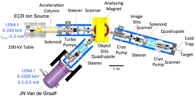
must be well defined, having a narrow energy distribution, and impinge upon the nuclear target in the presence of a γ-ray detector in order to observe and count the decay products of the reaction. The Laboratory for Experimental Nuclear Astrophysics (LENA) in Durham, North Carolina, is a unique facility designed specifically to excel at these types of measurements.
LENA is located on the campus of Duke University in Durham, NC, and is part of the Tri-angle Universities Nuclear Laboratory (TUNL). It is dedicated primarily to the study of nuclear cross sections at energies corresponding to the those relevant to nucleosynthesis in astrophysical processes. These take place in stellar environments at energies far too low for most accelerator facilities to probe effectively. The difficulties lie in the reduced transmission probability due to the Coulomb barrier, which suppresses the reaction signal below the limits of most detector systems. To counteract this effect, LENA employs two high-current proton accelerators in conjunction with a low-background γγ-coincidence spectrometer. These two features work in tandem, boosting the total number of reactions taking place while reducing the presence of environmental background to enhance signal detection. A schematic of the LENA facility is shown in Figure 4.1. The accel-erators, the 1 MV JN Van de Graaff (LENA I) and the 240 kV ECR ion source (LENA II) share an analyzing dipole magnet, which transports proton beam to the target station. Each segment of the beam-line has electromagnetic steerers and quadrupoles for directing and focusing the beam. Not shown in the diagram is the detector system, which is placed in close proximity to the target station in order to maximize the detection efficiency. The JN was used exclusively for this experi-ment, since the reference resonance,Elab
r = 619.6±1.2 keV [Kuperuset al.,1959], and those being
measured, the previously unobserved Elab
r = 435±4 keV [Vernotte et al., 1990] resonance and
Elab
p = 498.3±1.0 keV [Kuperus et al.,1959] resonance, lie within its energy range. Information
JN accelerator, the target station, and the detector system will now each be described.
Figure 4.1: A top-level view of LENA. The two proton accelerators, the 1 MV JN Van de Graaff (LENA I) and the 240 kV ECR ion source (LENA II), transport beam to a shared dipole magnet, which momentum analyses and bends it towards the target station. On each segment of the beam-line there are electromagnetic steerers and quadrupoles for beam shaping. Image courtesy of Art Champagne.
Section 4.1: LENA I, the JN Van de Graff
LENA I is an upgraded High Voltage Engineering Corporation 1 MV model JN Van de Graaff accelerator. It can produce up to≈150µA of H+ at energies between≈0.15−1 MeV. There have
a new acceleration column and charging belt. Recently, the Terminal Potential Stabilizer (TPS) system has been upgraded to a model TPS-6 fromNational Electrostatics Corp., which considerably improved the stability and precision of the beam-energy over previous studies using this facility. As a point of comparison, the full width at half maximum of the beam-energy profile observed during this dissertation was only 0.8 keV, several times smaller than the 2-3 keV spread observed inBuckner[2014].
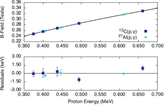
Prior to the resonance measurements, the JN was physically realigned with the dipole magnet as part of a campaign to improve beam transport, thereby invalidating the magnet calibration used in previous experiments. An accurate magnet calibration is necessary to measure resonance energies and make certain that the proton beam is probing the target layer at the right depth. The bending magnetic field associated with the energy of the beam,E, produced by the JN is given by
Iliadis [2015]:
B = k q
p
2mc2E+E2 (4.1)
wheremc2 andq are the rest mass and charge state of the ion, respectively. The constant, k, is
de-pendent on the trajectory of the beam through the magnet and must be determined by calibration. To calibrate the dipole magnet, the magnetic field strength corresponding to the energies of three well-known resonances in the 27Al(p,γ)28Si reaction was measured using yield curve analysis (see
Section 6.2). Several measurements were also made using the12C(p,γ)13N reaction, which produces
a γ-ray with an energy that is determined by the energy of the proton beam. Table 4.1 lists the measured resonances and direct capture energies used in the calibration and their associated mag-netic field measurements. These values are plotted in the top panel of Figure 4.2. The solid-line represents the fit of the data using Equation 4.1. In the lower-panel, the residual for each point, the experimentally observed energy minus the best fit result, is shown. In general there is good agreement between data sets, though the 12C capture data have a larger scatter, particularly at
Reaction Elab
p (keV) B-Field (Tesla)
27Al(p,γ)28Si 405.5±0.3 0.25857
446.7±0.5 0.27125
611.46±0.04 0.31753
12C(p,γ)13N 375.0±0.5 0.24858
400.1±0.8 0.25674
437.4±0.8 0.26837
493.4±0.4 0.28564
661.0±0.4 0.32988
Table 4.1: Dipole magnet calibration data obtained from the
27Al(p,γ)28Si and 12C(p,γ)13N reactions. Resonance energies and their
uncertainties for the27Al(p,γ) resonances are adopted fromEndt[1990].
For the12C(p,γ) data, energies and their uncertainties were determined
by a fit to spectroscopic data.
Figure 4.2: A fit of the dipole magnet calibration data. (Top Panel) The magnetic field strength required to transport the proton beam for each datum listed in Table 4.1 is plotted. (Bottom Panel) The deviation of each point from the best fit line is shown.
Section 4.2: The Target Station
with two goals in mind: the realization of a high vacuum, contaminant free environment, and the minimization of error in the incident charge measurement. Towards the fulfillment of the first goal, running along the length of the target station is a copper tube cold trap, cooled to liquid nitrogen temperature to minimize the migration of gaseous contaminants onto the surface of the target. The cold trap also contains a copper collimator with a diameter of 9.5 mm, which serves to limit the target area exposed to the beam. This also prevents charge accumulation on unimplanted or inert regions of the target. Below the cold-trap is a turbo-molecular pump, backed by an oil-free scroll pump. The combined effect of these two elements is a vacuum pressure of 1−2×10⁻⁷ Torr during
operation. The primary source of error in charge integration is the emission of secondary electrons on the surface of the target, which are knocked out by the incident proton beam and contribute to the current measured on target. To halt these electrons, a suppressing electric field is created by biasing an electrically isolated copper ring at the end of the cold-trap to −300 V. Finally, as a further measure to improve charge collection, the water used to cool the target is deionized.
Section 4.3: The γγ-Coincidence Spectrometer
Broadly speaking, the premise of a resonance yield measurement is to count the number of reactions that have taken place per incident particle. In the previous section, we saw how the incident protons can be counted using a specially designed Faraday cup. To count the nuclear reactions taking place, we rely on the nuclear deexcitations of the daughter nuclei produced in the reaction. In the case of 30Si(p,γ)31P, the excited 31P nucleus decays quickly (τ ≈ fs), emitting
one or more γ-rays until it is in the ground-state. In the presence of a radiation detector, these γ-rays can be counted to estimate the number of reactions taking place. However, other sources of radiation such as environmental background or beam-induced contaminant reactions often drown out the desired signal, requiring higher rates of data collection to achieve acceptable statistics. Theγγ-coincidence spectrometer employed at LENA was designed specifically to address this issue [Longlandet al.,2006].
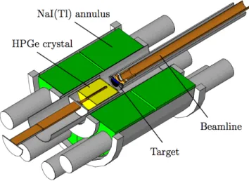
The system comprises a 135% high-purity germanium (HPGe) detector, oriented at 0◦ with respect to the beam axis, surrounded by a 16-segment NaI(Tl) annulus. These are enclosed in a lead shield, which is in turn surrounded by five sides of plastic scintillator paddles. A rendering of the detector system, shown in Figure 4.4, illustrates its geometry with respect to the target chamber, which is in contact with the HPGe crystal for maximum detection efficiency. Each segment of the NaI(Tl) annulus is optically isolated, allowing them to function independently. This setup is designed to exploitγ-ray cascade detection by using the peripheral energy deposition in the NaI(Tl) segments to classify HPGe events. An illustration of this is shown in Figure 4.5. Consider the reaction, X(p,γ)Y, which gives rise to an immediate two-stepγ-ray cascade, depositing γ12 (6 MeV) and γ10 (3 MeV) in the HPGe and NaI(Tl) annulus respectively. The events are
then plotted in the two-dimensional energy spectrum. By demanding that each HPGe event be accompanied by a NaI(Tl) event, with the further stipulation that the summed deposition energy, EHPGe+ENaI, falls between 5 and 10 MeV, an HPGe coincidence spectrum can be recorded, which
the use of the scintillator paddles, which are used in anti-coincidence mode to actively veto muon-induced events. The use of this spectrometer for γγ-coincidence spectroscopy has been reported previously inBuckneret al.[2015,2012], Cesarattoet al.[2013]. A more detailed description ofγγ techniques employed at LENA is given inLonglandet al. [2006].
Figure 4.4: The LENAγγ-coincidence spectrometer. A 135% HPGe detector (yellow) is surrounded by a 16-segment Na(Tl) annulus (green). The HPGe is put directly in contact with the target chamber for maximum efficiency. Not shown is the lead shield and plastic scintillator paddles. Figure fromDermigny et al.[2016]
4.3.1: Detection Efficiencies
The response of the HPGe detector to incident radiation is dependent on the geometry of the crystal (e.g., length, diameter) and also the geometry of the detector-target set-up. In a typical counting experiment, these figures are not known precisely. Instead, the peak efficiency of the detector,ηp, given by [Knoll, 2002]:
ηp = net intensity of full-energy peak
number ofγ-rays emitted by source , (4.2)
Figure 4.5: An illustration of the γγ-coincidence spectrometer gating scheme. The example reac-tion, X(p,γ)Y, initiates the two step γ-ray cascade, depositing γ12 and γ10 in the HPGe (yellow)
and NaI(Tl) annulus (green) respectively. By keeping only the events that fall between the dotted lines on the 2-d spectrum, the background can be reduced by several orders of magnitude.
its usefulness is limited when we consider its application to γγ-spectrometry. In a coincidence spectrum, the net intensity of a full-energy peak is dependent not only on the detection efficiency of that specificγ-ray, but on the detection efficiency of all otherγ-rays in that cascade with regard to the entire NaI(Tl) annulus. At LENA, this problem is circumvented using a high-fidelity simulation of the γγ-coincidence spectrometer.
Written using the detector simulation toolkit, Geant4 [Agostinelli et al., 2003], the program LENAGe uses precise measurements of the detector system geometry, as well as the details of the decay scheme, to generate the two-dimensional EHPGe versus ENaI spectrum seen in Figure 4.5. By
detector efficiencies and those simulated using LENAGe, which will serve as a proof-of-concept for the discussion later.
Research featuring theLENAGeprogram has been reported previously inLonglandet al. [2006],
Howard et al. [2013] and Dermignyet al. [2016]. The simulated HPGe detector geometry is based on measurements made by Carson et al. [2010]. In that work, computed tomography was used to determine the internal dimensions of the detector, such as the crystal length and diameter. For the NaI(Tl) annulus, the dimensions are based on information provided by the manufacturer. Several tests of the accuracy of the simulations have also been made. In Howard et al. [2013], a spectrum was taken from a calibrated22Na source and compared to a simulated singles spectrum,
normalized to the equivalent number of decays. The simulated and measured intensities of the full-energy 1275-keV peak were in agreement, to within 2% error, suggesting that the simulated HPGe detector response is accurate. The simulated NaI(Tl) response was then studied by applying a coincidence gate with the condition that the NaI(Tl) fully detects two 511-keV γ-rays emitted during the decay. The simulated and measured coincidence intensity of the 1275-keV peak were again in agreement to within 3% error.
To compare the simulated and observed detector response for the present experiment, an ab-solute efficiency calibration was performed using the sum-peak method [Kim et al., 2003]. This procedure takes advantage of the two-step γ-ray cascade following 60Co(β−ν¯
e)60Ni decay to
pro-vide peak efficiencies that are independent of the source activity. Consider the predominant decay channel (99.98%) of deexciting 60Ni nucleus, which can be represented by the following notation,
2→1→0, where 2→1 is the primary γ-ray (E21= 1173.228(3) keV) and 1→0 is the secondary
(E10= 1332.501(5) keV). In close geometries, these two coincidentγ-rays can sum together in the
detector to form a sum-peak at E20 = 2505.7 keV. The sum-peak method then yields the peak
efficiencies for the primary and secondary γ-rays:
ηp21= 1 W(θ)
s
N21N202
N10N20Nt+N21N102
(4.3)
ηp10= 1 W(θ)
s
N10N202
N21N20Nt+N10N212
, (4.4)
background-corrected total intensity, and W(θ) is the angular correlation of the two emitted photons. W(θ) is determined by the angular momenta of the decaying states and also the geometry of the detector. It is given by the expression [Iliadis, 2015]:
W(θ) = 1 + 5 49Q
10
2 Q212 P2(cosθ) +
4 411Q
10
4 Q214 P4(cosθ), (4.5)
whereP2 and P4 are the 2nd and 4th order Legendre polynomials, and the Qijk are the solid angle
attentuation factors for each γ-ray, γij. These were calculated for γ21 and γ10 using LenaGe by
simulating the isotropic emission of γ-rays in the same geometry. For each of the N detected (simulated) γ-rays in their respective full-energy peaks, the attenuation factors were given by:
Qijk = 1 N
N
X
l=0
Pkcosθl, (4.6)
where the θ is the emission angle with respect to the beam-axis for each photon that contributes to the full-energy photopeak.
This procedure was carried out using a60Co source (sealed in a mylar puck), which was fixed to
the inside of the target station end-cap at atmospheric pressure. Theγγ-coincidence spectrometer was then placed in the run geometry while a singles spectrum was collected over several hours. The net intensities of the three full-energy peaks were recorded and Equations 4.3 and 4.4 were used to calculate the peak efficiencies for γ21 and γ10, assuming emission from a “puck” source. The
obtained values were:
η21p (1173.2 keV) = 0.0379±0.0009 η10p (1332.5 keV) = 0.0352±0.0008,
fine-tuning the HPGe crystal geometry within the uncertainties published by Carsonet al. [2010]. For tables detailing the adopted crystal geometry values and the simulated efficiencies and attenuation coefficients, see Appendix B.1.
Using the same crystal geometry, the peak efficiencies were then calculated for a “beam-spot” configuration, which assumes that theγ-rays are emitted from a 9.5 mm diameter circular area on the face of the tantalum target, the same area of the target exposed to proton beam. In Figure 4.6, these are represented by the solid black line. To verify the shape of the efficiency curve, several well-known reactions were studied. Pulse-height spectra were recorded for the 56Co(e−, ν)56Fe decay
reaction using a puck source, and also the Elab
r = 278.0±0.3 keV resonance in14N(p,γ)15O [Daigle
et al.,2016] and the Elab
r = 405.5±0.3 keV resonance in the 27Al(p,γ)28Si reaction [Meyer et al., 1975] using proton beam from the JN. Peak efficiencies for the observed full-energy photopeaks were then calculated using the coincidence summing correction procedure outlined in Semkow et al. [1990]. A description of the code used to implement this method is given in Appendix C. It is similar to the sum-peak method, but is applicable to more generalized decays, those with multiple levels, feeding fractions, and branching ratios. The trade-off is that precise peak efficiencies cannot be calculated without a precisely known source activity, which is difficult to obtain for both puck sources and beam-induced resonance reactions. The peak efficiencies from these reactions therefore cannot be considered to be absolute calibrations. Instead, they are scaled to agree with the beam-spot efficiency curve predicted by LENAGe. Their agreement with the trend of the peak efficiency curve in Figure 4.6, in addition to those efficiencies derived using the sum-peak method, serve to corroborate the accuracy of the simulations. For the data analysis in this dissertation, a conservative systematic error of±4% is assumed for the full-energy peak efficiencies for data taken in singles mode. This interval is shown as a gray band around the beam-spot efficiency function.
Figure 4.6: A comparison of the simulated versus measured full-energy peak efficiencies for the source “puck” geometry (dashed line) and the beam-spot geometry (solid line). The efficiency of a γ-ray emitted in the beam-spot geometry is 11% greater than that of the puck geometry. The 60Co
efficiencies are absolute measurements determined using the sum-peak method. They are shown as solid black triangles. The 56Co, 14N(p,γ)15O, and 27Al(p,γ)28Si efficiency data are normalized to
the simulated beam-spot efficiencies.
the coincidence response metric,Cp, as:
Cp= (N
coin Geant/N
sing Geant)
(Ncoin
Obs / N
sing Obs)
(4.7)
where theN are the singles and coincidence net-intensities of a full-energy peak, obtained through experiment (“Obs”) and simulation (“Geant”). If the simulated γγ-spectrometer behaves identi-cally to the real system, then Cp would be unity. Using the same resonance reaction andβ-decay
data as in the HPGe efficiency measurements, Cp was measured for the same set of γ-ray
tran-sitions. A spectrum from the 22Na(β+ν)22Ne reaction was also included. For the coincidence
spectra, several different gating schemes were used. For the 56Co, 60Co, and 22Na β-decay data,
the gate was set so that all coincidences, regardless of the deposited energies, were accepted. For the14N(p,γ)15O resonance reaction, with a deexcitation energy of 7.556 MeV [Daigle et al.,2016],
the gate was set so that 3.0 < EHPGe + ENaI < 10.0 MeV. Finally, for the 27Al(p,γ)28Si
reso-nance reaction, with a deexcitation energy of 11.976 MeV [Meyer et al., 1975], the gate was set to 3.0 <EHPGe+ ENaI <14.0 MeV. The measured Cp values are shown in Figure 4.7, where the
lowest-energy points, the general trend suggests that the detector system is well modeled. Disre-garding these two outliers, the average coincidence response,Cp, over the energy range from 1 MeV
to 8 MeV, is 1.012±0.003. Since this is in such close agreement with the ideal case, no additional systematic error is assumed for the analysis of coincidence spectra in this dissertation. Instead, for both the singles and coincidence mode spectra, the adopted systematic error is determined solely by that of the HPGe crystal efficiencies, i.e., a conservative±4% error. This interval is shown as a gray band, centered at unity.
For the measurements in this dissertation, an intense proton beam and state-of-the-art detector system is necessary in order to obtain sufficient count rates. In this chapter, the instruments used at LENA and their role in this project were described. In particular, we looked at theγγ-coincidence spectrometer employed at LENA and the Geant4 simulation used to predict its response to γ -rays. Measurements of the peak efficiency function in singles mode corroborate the accuracy of the simulations with regard to the HPGe crystal. To validate coincidence mode simulations, we defined and studied a response metric based on the observed and simulatedγ-ray cascades and found that the predicted coincidence spectra were in close agreement with observations. In the next chapter, the use of these simulations to analyze pulse height spectra is described in detail.