DOI:10.1051/0004-6361/201424166 c
ESO 2014
Astrophysics
&
Shockingly low water abundances in
Herschel/PACS
observations of low-mass protostars in Perseus
A. Karska
1,2,3, L. E. Kristensen
4, E. F. van Dishoeck
1,2, M. N. Drozdovskaya
2, J. C. Mottram
2, G. J. Herczeg
5,
S. Bruderer
1, S. Cabrit
6, N. J. Evans II
7, D. Fedele
1, A. Gusdorf
8, J. K. Jørgensen
9,10, M. J. Kaufman
11, G. J. Melnick
3,
D. A. Neufeld
12, B. Nisini
13, G. Santangelo
13, M. Tafalla
14, and S. F. Wampfler
9,101 Max-Planck Institut für Extraterrestrische Physik (MPE), Giessenbachstr. 1, 85748 Garching, Germany e-mail:agata.karska@gmail.com
2 Leiden Observatory, Leiden University, PO Box 9513, 2300 RA Leiden, The Netherlands 3 Astronomical Observatory, Adam Mickiewicz University, Słoneczna 36, 60-268 Pozna´n, Poland 4 Harvard-Smithsonian Center for Astrophysics, 60 Garden Street, Cambridge, MA 02138, USA
5 Kavli Institut for Astronomy and Astrophysics, Yi He Yuan Lu 5, HaiDian Qu, Peking University, 100871 Beijing, PR China 6 LERMA, UMR 8112 du CNRS, Observatoire de Paris, École Normale Supérieure, Université Pierre et Marie Curie,
Université de Cergy-Pontoise, 61 Av. de l’Observatoire, 75014 Paris, France
7 Department of Astronomy, The University of Texas at Austin, 2515 Speedway, Stop C1400, Austin, TX 78712-1205, USA 8 LERMA, UMR 8112 du CNRS, Observatoire de Paris, École Normale Supérieure, 24 rue Lhomond, 75231 Paris Cedex 05, France 9 Niels Bohr Institute, University of Copenhagen, Juliane Maries Vej 30, 2100 Copenhagen Ø., Denmark
10 Centre for Star and Planet Formation, Natural History Museum of Denmark, University of Copenhagen, Øster Voldgade 5-7, 1350 Copenhagen K., Denmark
11 Department of Physics, San Jose State University, One Washington Square, San Jose, CA 95192-0106, USA
12 Department of Physics and Astronomy, Johns Hopkins University, 3400 North Charles Street, Baltimore, MD 21218, USA 13 INAF – Osservatorio Astronomico di Roma, 00040 Monte Porzio Catone, Italy
14 Observatorio Astronómico Nacional (IGN), Calle Alfonso XII,3. 28014 Madrid, Spain
Received 9 May 2014/Accepted 15 September 2014
ABSTRACT
Context.Protostars interact with their surroundings through jets and winds impinging on the envelope and creating shocks, but the nature of these shocks is still poorly understood.
Aims.Our aim is to survey far-infrared molecular line emission from a uniform and significant sample of deeply-embedded low-mass young stellar objects (YSOs) in order to characterize shocks and the possible role of ultraviolet radiation in the immediate protostellar environment.
Methods.Herschel/PACS spectral maps of 22 objects in the Perseus molecular cloud were obtained as part of theWilliam Herschel Line Legacy (WILL) survey. Line emission from H2O, CO, and OH is tested against shock models from the literature.
Results.Observed line ratios are remarkably similar and do not show variations with physical parameters of the sources (luminosity, envelope mass). Most ratios are also comparable to those found at off-source outflow positions. Observations show good agreement with the shock models when line ratios of the same species are compared. Ratios of various H2O lines provide a particularly good diagnostic of pre-shock gas densities,nH ∼105 cm−3, in agreement with typical densities obtained from observations of the post-shock gas when a compression factor on the order of 10 is applied (for non-dissociative post-shocks). The corresponding post-shock velocities, obtained from comparison with CO line ratios, are above 20 km s−1. However, the observations consistently show H
2O-to-CO and H2O-to-OH line ratios that are one to two orders of magnitude lower than predicted by the existing shock models.
Conclusions.The overestimated model H2O fluxes are most likely caused by an overabundance of H2O in the models since the excitation is well-reproduced. Illumination of the shocked material by ultraviolet photons produced either in the star-disk system or, more locally, in the shock, would decrease the H2O abundances and reconcile the models with observations. Detections of hot H2O and strong OH lines support this scenario.
Key words.astrochemistry – stars: formation – ISM: jets and outflows
1. Introduction
Shocks are ubiquitous phenomena where outflow-envelope in-teractions take place in young stellar objects (YSO). Large-scale shocks are caused by the bipolar jets and protostellar winds im-pinging on the envelope along the cavity walls carved by the
Appendices are available in electronic form at http://www.aanda.org
passage of the jet (Arce et al. 2007; Frank et al. 2014). This important interaction needs to be characterized in order to un-derstand and quantify the feedback from protostars onto their surroundings and, ultimately, to explain the origin of the initial mass function, disk fragmentation, and the binary fraction.
Theoretically, shocks are divided into two main types based on a combination of magnetic field strength, shock velocity, density, and level of ionization (Draine 1980; Draine et al. 1983;Hollenbach et al. 1989;Hollenbach 1997). In continuous
(C-type) shocks, in the presence of a magnetic field and low ionization, the weak coupling between the ions and neutrals re-sults in a continuous change in the gas parameters. Peak temper-atures of a few 103K allow the molecules to survive the passage of the shock, which is therefore referred to as non-dissociative. In jump (J-type) shocks, physical conditions change in a dis-continuous way, leading to higher peak temperatures than in Cshocks of the same speed and for a given density. Depending on the shock velocity, J shocks are either non-dissociative (velocities below about ∼30 km s−1, peak temperatures of a few 104 K) or dissociative (peak temperatures even exceeding 105 K), but the molecules efficiently reform in the post-shock gas.
Shocks reveal their presence most prominently in the in-frared (IR) domain, where the post-shock gas is efficiently cooled by numerous atomic and molecular emission lines. Cooling from H2 is dominant in outflow shocks (Nisini et al. 2010b;Giannini et al. 2011b), but its mid-IR emission is strongly affected by extinction in the dense envelopes of young proto-stars (Giannini et al. 2001a;Nisini et al. 2002;Davis et al. 2008; Maret et al. 2009). In the far-IR, rotational transitions of water vapor (H2O) and carbon monoxide (CO) are predicted to play an important role in the cooling process (Goldsmith & Langer 1978; Neufeld & Dalgarno 1989; Hollenbach 1997) and can serve as a diagnostic of the shock type, its velocity, and the pre-shock density of the medium (Hollenbach et al. 1989;Kaufman & Neufeld 1996;Flower & Pineau des Forêts 2010,2012).
The first observations of the critical wavelength regime to test these models (λ∼45−200μm) were taken using the Long-Wavelength Spectrometer (LWS,Clegg et al. 1996) on board the Infrared Space Observatory (ISO,Kessler et al. 1996). Far-IR atomic and molecular emission lines were detected toward sev-eral low-mass deeply-embedded protostars (Nisini et al. 2000; Giannini et al. 2001a;van Dishoeck 2004), but its origin was unclear because of the poor spatial resolution of the telescope (∼80,Nisini et al. 2002;Ceccarelli et al. 2002).
The sensitivity and spectral resolution of the Photodetector Array Camera and Spectrometer (PACS,Poglitsch et al. 2010) on boardHerschel allowed a significant increase in the num-ber of detections of far-IR lines in young protostars compared with the early ISO results and has revealed rich molecular and atomic line emission both at the protostellar (e.g.,van Kempen et al. 2010;Goicoechea et al. 2012;Herczeg et al. 2012;Visser et al. 2012;Green et al. 2013;Karska et al. 2013;Lindberg et al. 2014;Manoj et al. 2013;Wampfler et al. 2013) and at pure out-flow positions (Santangelo et al. 2012,2013;Codella et al. 2012; Lefloch et al. 2012a;Vasta et al. 2012;Nisini et al. 2013).
The unprecedented spatial resolution of PACS allowed de-tailed imaging of L1157 providing firm evidence that most far-IR H2O emission originates in the outflows (Nisini et al. 2010a). A mapping survey of about 20 protostars revealed sim-ilarities between the spatial extent of H2O and high-J CO (Karska et al. 2013). Additional strong flux correlations be-tween these species and similarities in the velocity-resolved pro-files (Kristensen et al. 2010,2012;San José-García et al. 2013; Santangelo et al. 2014) suggest that the emission from the two molecules arises from the same regions. This is further con-firmed by finely-spatially sampled PACS maps in CO 16−15 and various H2O lines in shock positions of L1448 and L1157 (Santangelo et al. 2013;Tafalla et al. 2013). On the other hand, the spatial extent of OH resembles the extent of [O
i
] and, ad-ditionally, a strong flux correlation between the two species is found (Karska et al. 2013; Wampfler et al. 2013). Therefore, at least part of the OH emission most likely originates in adissociativeJ-shock, together with [O
i
] (Wampfler et al. 2010, 2013;Benedettini et al. 2012).To date, comparisons of the far-IR observations with shock models have been limited to a single source or its outflow po-sitions (e.g.,Nisini et al. 1999; Benedettini et al. 2012; Vasta et al. 2012; Santangelo et al. 2012; Dionatos et al. 2013;Lee et al. 2013;Flower & Pineau des Forêts 2013). Even in these studies, separate analysis of each species (or different pairs of species) often led to different sets of shock properties that needed to be reconciled. For example,Dionatos et al.(2013) show that CO and H2 line emission in Serpens SMM3 originates from a 20 km s−1 Jshock at low pre-shock densities (∼104 cm−3), but the H2O and OH emission is better explained by a 30−40 km s−1 C shock. In contrast,Lee et al.(2013) associate emission from both CO and H2O in L1448-MM with a 40 km s−1 Cshock at high pre-shock densities (∼105cm−3), consistent with the anal-ysis of the L1448-R4 outflow position (Santangelo et al. 2013). Analysis restricted to H2O lines alone often indicates an origin in non-dissociativeJshocks (Santangelo et al. 2012;Vasta et al. 2012;Busquet et al. 2014), while separate analysis of CO, OH, and atomic species favors dissociative J shocks (Benedettini et al. 2012; Lefloch et al. 2012b). The question remains how to break degeneracies between these models and how typical the derived shock properties are for young protostars. In addition, surveys of high-JCO lines with PACS have revealed two univer-sal temperature components in the CO ladder toward all deeply-embedded low-mass protostars (Herczeg et al. 2012;Goicoechea et al. 2012; Green et al. 2013;Karska et al. 2013;Kristensen et al. 2013;Manoj et al. 2013;Lee et al. 2013). The question is how the different shock properties relate with the “warm” (T ∼ 300 K) and “hot” (T 700 K) components seen in the CO rotational diagrams.
In this paper, far-IR spectra of 22 low-mass YSOs observed as part of theWilliam HerschelLine Legacy (WILL) survey (PI: E. F. van Dishoeck) are compared to the shock models from Kaufman & Neufeld(1996) and Flower & Pineau des Forêts (2010). All sources are confirmed deeply-embedded YSOs lo-cated in the well-studied Perseus molecular cloud spanning the Class 0 and I regime (Knee & Sandell 2000;Enoch et al. 2006, 2009;Jørgensen et al. 2006,2007;Hatchell et al. 2007a,b;Davis et al. 2008;Arce et al. 2010). H2O, CO, and OH lines are ana-lyzed together for this uniform sample to answer the following questions: Do far-IR line observations agree with the shock mod-els? How much variation in observational diagnostics of shock conditions is found between different sources? Can one set of shock parameters explain all molecular species and transitions? Are there systematic differences between shock characteristics inferred using the CO lines from the “warm” and “hot” compo-nents? How do shock conditions vary with the distance from the powering protostar?
This paper is organized as follows. Section 2 describes our source sample, instrument with adopted observing mode, and reduction methods. Section 3 presents the results of the obser-vations: line and continuum maps, and the extracted spectra. Section 4 shows comparison between the observations and shock models. Section 5 discusses results obtained in Sects. 4 and 6 presents the conclusions.
2. Observations
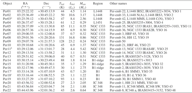
Table 1.Catalog information and source properties.
Object RA Dec Tbol Lbol Menv Region Other names
(h m s) (◦ ) (K) (L
) (M)
Per01 03:25:22.32 +30:45:13.9 44 4.5 1.14 L1448 Per-emb 22, L1448 IRS2, IRAS03222+3034, YSO 1 Per02 03:25:36.49 +30:45:22.2 50 10.6 3.17 L1448 Per-emb 33, L1448 N(A), L1448 IRS3, YSO 2 Per03a 03:25:39.12 +30:43:58.2 47 8.4 2.56 L1448 Per-emb 42, L1448 MMS, L1448 C(N), YSO 3 Per04 03:26:37.47 +30:15:28.1 61 1.2 0.29 L1451 Per-emb 25, IRAS03235+3004, YSO 4
Per05 03:28:37.09 +31:13:30.8 85 11.1 0.35 NGC 1333 Per-emb 35, NGC 1333 IRAS1, IRAS03255+3103, YSO 11 Per06 03:28:57.36 +31:14:15.9 85 6.9 0.30 NGC 1333 Per-emb 36, NGC 1333 IRAS2B, YSO 16
Per07 03:29:00.55 +31:12:00.8 37 0.7 0.32 NGC 1333 Per-emb 3, HRF 65, YSO 18 Per08 03:29:01.56 +31:20:20.6 131 16.8 0.86 NGC 1333 Per-emb 54, HH 12, YSO 19 Per09 03:29:07.78 +31:21:57.3 128 23.2 0.24 NGC 1333 Per-emb 50
Per10 03:29:10.68 +31:18:20.6 45 6.9 1.37 NGC 1333 Per-emb 21, HRF 46, YSO 23
Per11b 03:29:12.06 +31:13:01.7 28 4.4 5.42 NGC 1333 Per-emb 13, NGC 1333 IRAS4B, YSO 25 Per12 03:29:13.54 +31:13:58.2 31 1.1 1.30 NGC 1333 Per-emb 14, NGC 1333 IRAS4C, YSO 26 Per13 03:29:51.82 +31:39:06.0 40 0.7 0.51 NGC 1333 Per-emb 9, IRAS03267+3128, YSO 31 Per14 03:30:15.14 +30:23:49.4 88 1.8 0.14 B1-ridge Per-emb 34, IRAS03271+3013 Per15 03:31:20.98 +30:45:30.1 35 1.7 1.29 B1-ridge Per-emb 5, IRAS03282+3035, YSO 32 Per16 03:32:17.96 +30:49:47.5 30 1.1 2.75 B1-ridge Per-emb 2, IRAS03292+3039, YSO 33 Per17c 03:33:14.38 +31:07:10.9 43 0.7 1.20 B1 Per-emb 6, B1 SMM3, YSO 35 Per18c 03:33:16.44 +31:06:52.5 25 1.1 1.22 B1 Per-emb 10, B1 d, YSO 36 Per19 03:33:27.29 +31:07:10.2 93 1.1 0.23 B1 Per-emb 30, B1 SMM11, YSO 40 Per20 03:43:56.52 +32:00:52.8 27 2.3 2.05 IC 348 Per-emb 1, HH 211 MMS, YSO 44
Per21 03:43:56.84 +32:03:04.7 34 2.1 1.88 IC 348 Per-emb 11, IC348 MMS, IC348 SW, YSO 43 Per22 03:44:43.96 +32:01:36.2 43 2.6 0.64 IC 348 Per-emb 8, IC348 a, IRAS03415+3152, YSO 48
Notes.Bolometric temperatures and luminosities are determined including the PACS continuum values; the procedure will be discussed in Mottram et al. (in prep.). Numbered Per-emb names come fromEnoch et al.(2009), whereas the numbered YSO names come fromJørgensen et al.(2006) and were subsequently used inDavis et al.(2008). Other source identifiers were compiled usingJørgensen et al.(2007),Rebull et al.(2007),Davis et al.(2008), andVelusamy et al.(2014). Observations obtained in 2011 which overlap with Per03 and Per11 are presented inLee et al.(2013) and Herczeg et al.(2012), respectively.(a)Tabulated values come fromGreen et al.(2013), where full PACS spectra are obtained. The WILL values forTbolandLbolare 48 K and 8.0L, respectively, within 5% of those ofGreen et al.(2013).(b)Tabulated values come fromKarska et al.(2013) and agree within 2% of the values 29 K and 4.3Lobtained here. We prefer to use the previously published values because the pointing of that observation was better centered on the IRAS4B.(b) The off-positions of Per17 and Per18 were contaminated by other continuum sources, and therefore theTbolandLbolare calculated here without theHerschel/PACS points.
Instrument for the Far-Infrared (HIFI,de Graauw et al. 2010) toward an unbiased flux-limited sample of low-mass protostars newly discovered in the recentSpitzer (c2d,Gutermuth et al. 2009,2010;Evans et al. 2009) andHerschel(André et al. 2010) Gould Belt imaging surveys. Its main aim is to study the physics and chemistry of star-forming regions in a statistically signifi-cant way by extending the sample of low-mass protostars ob-served in the “Water in star-forming regions with Herschel” (WISH,van Dishoeck et al. 2011) and “Dust, Ice, and Gas in Time” (DIGIT,Green et al. 2013) programs.
This paper presents theHerschel/PACS spectra of 22 low-mass deeply-embedded YSOs located exclusively in the Perseus molecular cloud (see Table1) to ensure the homogeneity of the sample (similar ages, environment, and distance). The sources were selected from the combined SCUBA and Spitzer/IRAC and MIPS catalog ofJørgensen et al.(2007) andEnoch et al. (2009), and all contain a confirmed embedded YSO (Stage 0 or I, Robitaille et al. 2006,2007) in the center.
The WILL sources were observed using the line spec-troscopy mode on PACS which offers deep integrations and finely sampled spectral resolution elements (minimum 3 samples per FWHM depending on the grating order, PACS Observer’s Manual1) over short wavelength ranges (0.5−2μm). The line se-lection was based on the prior experience with the PACS spectra obtained over the full far-infrared spectral range in the WISH and DIGIT programs and is summarized in TableA.1. Details of
1 http://herschel.esac.esa.int/Docs/PACS/html/pacs_om.
html
the observations of the Perseus sources within the WILL survey are shown in TableA.2.
PACS is an integral field unit with a 5 × 5 array of spatial pixels (hereafter spaxels) covering a field of view of∼47×47. Each spaxel measured∼9.4 ×9.4, or 2 × 10⁻⁹ sr, and at the distance to Perseus (d = 235 pc, Hirota et al. 2008) re-solves emission down to ∼2300 AU. The total field of view is about 5.25×10⁻⁸ sr and ∼11 000 AU. The properly flux-calibrated wavelength ranges include:∼55−70μm,∼72−94μm, and ∼105−187 μm, corresponding to the second (<100 μm) and first spectral orders (>100μm). Their respective spectral resolving power are R ∼ 2500−4500 (velocity resolution of
Δ∼70−120 km s−1), 1500−2500 (Δ∼120−200 km s−1), and 1000−1500 (Δ ∼ 200−300 km s−1). The standard chopping-nodding mode was used with a medium (3) chopper throw. The telescope pointing accuracy is typically better than 2 and can be evaluated to first order using the continuum maps.
The basic data reduction presented here was performed us-ing theHerschelInteractive Processing Environment v.10 (
hipe
, Ott 2010). The flux was normalized to the telescopic background and calibrated using observations of Neptune. Spectral flatfield-ing within HIPE was used to increase the signal-to-noise (for details, seeHerczeg et al. 2012;Green et al. 2013). The overall flux calibration is accurate to∼20%, based on the flux repeata-bility for multiple observations of the same target in different programs, cross-calibrations with HIFI and ISO, and continuum photometry.Table 2.Notes on mapped regions for individual sources.
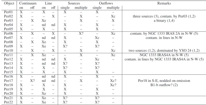
Object Continuum Line Sources Outflows Remarks
on off on off single multiple single multiple
Per01 X – X – X – X –
Per02 X – – X – X – Xc three sources (3), contam. by Per03 (1,2)
Per03 – X Xe – X – X a binary (1,4)
Per04 X – nd nd X – X –
Per05 X – X – X – X –
Per06 – X – X – X? – Xc contam. by NGC 1333 IRAS 2A in N-W (5)
Per07 X – nd nd X – Xc – contam. in lines in N-W
Per08 – X Xe – X – X –
Per09 X – Xe – X? – X? –
Per10 – X – X – X – Xc two sources (1,2), dominated by YSO 24 (1,2)
Per11 – X Xe – – X – Xc NGC 1333 IRAS4A in N-W (5)
Per12 X – nd nd X – Xc – contam. in lines by NGC 1333 IRAS4A in N-W (5)
Per13 X – nd nd X? – X?
Per14 X – X – X? – X?
Per15 X – X – X – X –
Per16 X – nd nd X – X –
Per17 – X? nd nd – X – Xc? Per18 in S-E, nodded on emission
Per18 X – X – X – – Xc? B1-b outflow? (2)
Per19 X – X – X – X –
Per20 X – Xe – X – X –
Per21 X – Xe – X? – X? –
Per22 X – Xe – X? – X? –
Notes.Columns 2–5 indicate the location of the continuum at 179μm and line emission peak of the H2O 212−101(179.527μm) transition on the maps (whether on or off-center). Columns 6−9 provide information about the number of sources and their outflows in the mapped region. Contamination by the outflows driven by sources outside the PACS field of view is mentioned in the last column. Extended emission associated with the targeted sources is denoted by “e”. Non-detections are abbreviated by “nd”, while “c” marks the contamination of the targeted source map by outflows from other sources.
References.(1)Jørgensen et al.(2006); (2)Davis et al.(2008); (3)Looney et al.(2000); (4)Hirano et al.(2010);Lee et al.(2013); (5)Yıldız et al. (2014).
co-adding spaxels with detected line emission, after exclud-ing contamination from other nearby sources except Per 2, 3, 10, and 18, where spatial separation between different com-ponents is too small (see Sect. 3.1). For sources showing ex-tended emission, the set of spaxels providing the maximum flux was chosen for each line separately. For point-like sources, the flux is calculated at the central position and then corrected for the PSF using wavelength-dependent correction factors (see PACS Observer’s Manual). TableA.3shows the line detections toward each source, while the actual fluxes will be tabulated in the forthcoming paper for all the WILL sources (Karska et al., in prep.). Fits cubes containing the spectra in each spaxel will be available for download in early 2015 athttp://www.strw.
leidenuniv.nl/WISH/.
3. Results
In the following sections, PACS lines and maps of the Perseus YSOs are presented. Most sources in this sample show emis-sion in just the central spaxel. Only a few sources show extended emission and those maps are compared to maps at other wave-lengths to check for possible contamination by other sources and their outflows. In this way, the spaxels of the maps with emission originating from our objects are established and line fluxes de-termined over those spaxels. The emergent line spectra are then discussed.
3.1. Spatial extent of line emission
Table2provides a summary of the patterns of H2O 212−101line and continuum emission at 179 μm for all WILL sources in Perseus (maps are shown in Figs.A.1andA.2). The mid-infrared
continuum and H2 line maps fromJørgensen et al.(2006) and Davis et al.(2008, including CO 3−2 observations fromHatchell et al. 2007a) are used to obtain complementary information on the sources and their outflows. For a few well-known outflow sources, large-scale CO 6−5 maps fromYıldız et al.(2014) are also considered.
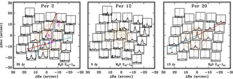
As shown in Table 2, the majority of the PACS maps to-ward Perseus YSOs do not show any extended line emission. The well-centered continuum and line emission originates from a single object and an associated bipolar outflow for 12 out of 22 sources. Among the sources with spatially-resolved extended emission on the maps, various reasons are identified for their ori-gin as illustrated in Fig.1. In the map of Per 2, contribution from three nearby protostars and a strong outflow from the more dis-tant L1448-MM source cause the extended line and continuum pattern. Emission in the Per 12 map is detected away from the continuum peak, but the emission originates from a large-scale outflow from NGC 1333-IRAS4A, not the targeted source. The H2O emission in the Per 20 map is detected in the direction of the strong outflow and its extent is only slightly affected by the small mispointing revealed by the asymmetric continuum emission.
Extended emission beyond the well-centered continuum, as in the case of Per 20, is seen clearly only in Per 9 and Per 21-22. Additionally, the continuum peaks for Per 3, 8, and 11 are off -center, whereas the line emission peaks on-source, suggesting that some extended line emission is associated with the source itself and not only due to the mispointing2. Similar continuum patterns are seen in Per 6 and Per 10, but here the line emission
Fig. 1.PACS spectral maps in the H2O 212−101line at 179μm illustrating sources with extended emission due to multiple sources in one field (Per 2), contamination by the outflow driven by another source (Per 12), and associated with the targeted protostar (Per 20). Even though the emission on the maps seems to be extended in many sources in Perseus, the extended emissionassociated with the targeted protostar itself is detected only towards a few of them (see Table 2). The orange contours show continuum emission at 30%, 50%, 70%, and 90% of the peak value written in the bottom left corner of each map. L1448 IRS 3A, 3B, and 3C sources and their CO 2−1 outflow directions are shown on the map of Per 2 (Kwon et al. 2006;Looney et al. 2000); the blue outflow lobe of L1448-MM also covers much of the observed field. CO 2−1 outflow directions of Per 20/HH211 are taken fromGueth & Guilloteau(1999). Wavelengths in microns are translated to the velocity scale on theX-axis using laboratory wavelengths (see TableA.1) of the species and cover the range from−600 to 600 km s−1. TheY-axis shows fluxes in Jy normalized to the spaxel with the brightest line on the map in a range−0.2 to 1.2.
peaks a few spaxels away from the map center. In both cases, contribution from additional outflows/sources is the cause of the dominant off-source line emission.
To summarize, when the contamination of other sources and their outflows can be excluded, Perseus YSOs show that the H2O 212−101 line emission is either well-confined to the cen-tral position on the map or shows at best weak extended line emission (those are marked with “e” in Table 2). In total, 7 out of 22 sources show extended emission in the H2O 212−101line associated with the targeted sources. Emission in CO, OH, and other H2O lines follows the same pattern (see Fig. A.3). Similarly compact emission was seen in a sample of 30 pro-tostars surveyed in the DIGIT program (Green et al. 2013). In contrast, the WISH PACS survey (Karska et al. 2013) revealed strong extended emission in about half of the 20 low-mass pro-tostars. There, the analysis of patterns of molecular and atomic emission showed that H2O and CO spatially co-exist within the PACS field of view, while OH and [O
i
] lines are typically less extended, but also follow each other spatially and not H2O and CO.3.2. Line detections
In the majority of our sources, all targeted rotational transitions of CO, H2O, and OH are detected, see Fig.2 and Tables A.1 andA.3. The [O
i
] line at 63μm and the [Cii
] line at 158μm will be discussed separately in a forthcoming paper including all WILL sources (Karska et al., and in prep.) and are not included in the figure and further analysis.The CO 16−15 line with an upper level energy (Eu/kB) of about 750 K is seen in 17 (∼80%), the CO 24−23 (Eu/kB ∼ 1700 K) in 16 (∼70%), and the CO 32−31 (Eu/kB ∼ 3000 K) in 8 (∼30%) sources. The most commonly detected ortho-H2O lines are: the 212−101 line at 179μm (Eu/kB∼110 K) and the 404−313line at 125μm (Eu/kB∼320 K), seen in 15 sources (∼70%), whereas the 616−505 line at 82μm (Eu/kB ∼ 640 K) is detected in 13 sources (∼60%). The para-H2O line 322−211at 90μm (Eu/kB∼300 K) is seen toward 9 sources (∼50%).
Three OH doublets targeted as part of the WILL survey, the OH2Π
1/2,J=1/2−2Π3/2,J=3/2at 79μm,2Π3/2J=7/2−5/2
dou-blet at 84μm (Eu/kB∼290 K), and2Π1
/2J=3/2−1/2doublet at
163μm (Eu/kB∼270 K), are detected in 14, 15, and 13 objects, respectively (∼60−70%).
Sources without any detections of molecular lines associ-ated with the targeted protostars are Per 4, 7, 12, and 17 (see Table A.3). In Per 13 only two weak H2O lines at 108 and 125μm are seen, whereas in Per 16 only a few of the lowest-J CO lines are detected. A common characteristic of this weak-line group of objects, is a low bolometric temperature (all ex-cept Per 4) and a low bolometric luminosity (see Table1), al-ways below 1.3L. However, our sample also includes a few objects with similarly low values ofLbol, that show many more molecular lines (in particular Per 3, but also Per 15 and 21), so low luminosity by itself is not a criterion for weak lines. On the other hand, low bolometric temperature and high luminosity is typically connected with strong line emission (Kristensen et al. 2012;Karska et al. 2013).
3.3. Observed line ratios
Fig. 2. Line survey of deeply-embedded young stellar objects in Perseus at the central position on the maps. Spectra are continuum subtracted and not corrected for the PSF. Line identification of CO (red), H2O (blue), and OH (light blue), are shown. Each spectrum is on a scale from 0 to 5 Jy in they-axis, with the brightest sources – Per 3, Per 9, and Per 11 – scaled down in flux density by a factor of 0.1, 0.5, and 0.1, respectively.
Fluxes of the nearby H2O 404−313 and CO 21−20 lines lo-cated at 124−125μm are calculated first using only the central spaxel (compact region) and then using all the spaxels with de-tected line emission (extended region). Figure3illustrates that the line ratios calculated in these two regions are fully con-sistent, both for sources with compact and extended emission. Therefore, for the subsequent analysis the extended region is used for comparisons with models. Table A.4shows the min-imum and maxmin-imum values of the observed line ratios, their mean values, and the standard deviations for all sources with detections.
Table 3.Comparison of observed H2O, CO, and OH line ratios with literature values.
Object 212−101/16−15 404−313/24−23 16−15/24−23 212−101/404−313 221−110/404−313 OH 84/79 Ref. Perseus (this work)
Perseus 0.2–2.4 0.2–1.1 1.2–4.6 1.3–6.3 1.4–5.5 1.1–2.4 This work
On–source (literature)
SMM3 b 1.0±0.1 0.5±0.2 3.3±0.8 7.1±1.0 3.7±1.0 1.4±0.7 (1) c 0.9±0.2 0.9±0.3 4.6±1.0 4.9±1.0 2.3±0.8 2.4±1.2 (1)
r 1.0±0.1 2.0±0.7 9.4±2.3 4.7±1.0 3.1±0.9 n.d. (1)
SMM4 r 0.8±0.1 0.4±0.1 3.6±0.6 7.8±1.6 3.0±1.3 1.1±0.5 (1) L1448-MM 2.3±1.3 1.2±0.7 2.1±1.2 4.1±2.3 2.6±1.5 1.4±0.9 (2) NGC 1333 I4B 1.0±0.1 1.0±0.1 1.9±0.1 1.9±0.1 2.0±0.1 1.2±0.2 (3)
Off–source (literature)
L1157 B1 4.0±0.5 – – 11.0 2.9±1.2 n.d. (4, 5)
B1 2.1±0.2 – – 9.2±2.2 2.8±1.0 0.9±0.5 (4, 5)
B2 17.0±8.4 n.d. >0.3 >7.7 n.d. – (6)
R 5.3±2.4 >0.26 >0.5 10.6±4.7 1.8±0.8 – (6)
L1448 B2 2.3±0.4 0.4±0.3 2.8±0.9 15.0±6.5 3.7±1.6 – (6)
R4 8.2±3.0 >0.3 >0.9 23.2±9.7 3.3±1.2 – (6)
Notes.Sources in the upper part of the table refer to protostellar positions within the PACS maps, sources in the lower part refer to shock positions away from the protostar. Ranges of line ratios calculated for Perseus sources are listed at the top. Line ratios of sources that exceed the Perseus values are shown in boldface. The L1157 B1 position refers to the high-excitation CO emission peak close to the nominal position of the B1 shock spot (Benedettini et al. 2012). Non-detections are abbreviated with n.d. OH 84/79 refers to the ratio of two OH doublets, at 84 and 79μm, respectively. The total flux of the 84μm doublet is calculated by multiplying the 84.6μm flux by two, because of the blending of the 84.4μm line with the CO 31−30 line.
References.(1)Dionatos et al.(2013); (2)Lee et al.(2013); (3)Herczeg et al.(2012); (4)Benedettini et al.(2012); (5)Busquet et al.(2014); (6) Santangelo et al.(2013).
Fig. 3. Flux ratios of the H2O 404−313and CO 21−20 lines at∼125μm
calculated usingcompactandextendedflux extraction regions (see text) corrected for contamination from other sources/outflows. Median val-ues for the two configurations are shown by the dashed line. The light blue rectangle shows the parameter space between the minimum and maximum values of line ratios in the more extended configuration. The error bars reflect the uncertainties in the measured fluxes of the two lines, excluding the calibration error, which is the same for those closely spaced lines.
Our line ratios for Perseus sources are consistent with the previously reported values for other deeply-embedded protostars observed in the same way (“on source”) as tabulated in Table3. Some differences are found for PACS observations of shock po-sitions away from the protostar (“offsource”). Most notably, the ratios using the low excitation H2O 212−101line at 179μm are up to a factor of two larger than those observed in the proto-stellar vicinity. Such differences are not seen when more highly-excited H2O lines are compared with each other, for example H2O 221−110and 404−313lines, or with the high-JCO lines, for example CO 24−23. The ratios of two CO lines observed away from the protostar, e.g., the CO 16−15 and CO 24−23 ratios,
are at the low end of the range observed toward the protostellar position.
Spectrally-resolved profiles of the H2O 212−101 line ob-served with HIFI toward the protostar position reveal absorp-tions at source velocity removing about 10% of total line flux (e.g.,Kristensen et al. 2010; Mottram et al. 2014). Our unre-solved PACS observations therefore provide a lower limit to the H2O emission in the 212−101 line. This effect, however, is too small to explain the differences in the line ratios at the “on source” and “offsource” positions.
4. Analysis
Multiple molecular transitions over a wide range of excitation energies are detected, which points to the presence of hot, dense gas and can be used to constrain the signatures of shocks cre-ated as a result of outflow-envelope interaction. In particular, the line ratios of H2O, CO, and OH are useful probes of vari-ous shock types and parameters that do not suffer from distance uncertainties.
Similarities between the spatial extent of different molecules (Sect. 3.1) coupled with similarities in the velocity-resolved line profiles among these species (Kristensen et al. 2010;Yıldız et al. 2013;San José-García et al. 2013;Mottram et al. 2014) strongly suggest that all highly-excited lines of CO and H2O arise from the same gas. Some differences may occur for OH, which is also associated with dissociative shocks and can be affected by radia-tive excitation (see Sect. 5). Modeling of absolute line fluxes re-quires sophisticated two-dimensional (2D) physical source mod-els for the proper treatment of the beam filling factor (Visser et al. 2012). Those models also show that UV heating alone is not sufficient to account for the high excitation lines. Hence, the focus in this analysis is on shocks. Since the absolute flux de-pends sensitively on the assumed emitting area, in the subse-quent analysis only the line ratios are compared.
(Sect. 4.1) and observations are compared with the models, using line ratios of the same species (Sect. 4.2), and different species (Sect. 4.3). Special focus will be given toC-type shocks where grids of model results are available in the literature. Observations suggest that most of the mass of hot gas is inC-type shocks toward the central protostellar positions, at least for H2O and CO withJ < 30 (Kristensen et al. 2013, and in prep.); higher-JCO, OH and [O
i
] transitions, on the other hand, will primarily traceJ-type shocks (e.g.,Wampfler et al. 2013;Kristensen et al. 2013). The excitation of OH and [Oi
] will be analyzed in a forth-coming paper; theJ >30 CO emission is only detected toward ∼30% of all sources and so is likely unimportant for the analy-sis and interpretation of the data presented here. Only a limited discussion ofJ-type shocks is therefore presented below.4.1. Model line emission
Models of shocks occurring in a medium with physical condi-tions typical for the envelopes of deeply-embedded young stel-lar objects provide a valuable tool for investigating shock char-acteristics: shock type, velocity, and the pre-shock density of (envelope) material.
Model grids have been published using a simple 1D geome-try either for steady-stateCandJtype shocks (Hollenbach et al. 1989;Kaufman & Neufeld 1996;Flower & Pineau des Forêts 2010) or time-dependentC−Jtype shocks (Gusdorf et al. 2008, 2011;Flower & Pineau des Forêts 2012). The latter are non-stationary shocks, where aJ-type front is embedded in aC-type shock (Chieze et al. 1998;Lesaffre et al. 2004a,b). These shocks are intermediate between pureC- and J-type shocks and have temperatures and physical extents in between the two extremes. C-Jshocks may be required for the youngest outflows with ages less than 103yrs, (Flower & Pineau des Forêts 2012,2013, for the case of IRAS4B, Per 11). Here the dynamical age of the outflow is taken as an upper limit of that of the shock itself, which may be caused by a more recent impact of the wind on the envelope. The age of our sources is on the order of 105yrs (Sadavoy et al. 2014, for Class 0 sources in Perseus) and they should have been driving winds and jets for the bulk of this pe-riod, so this timescale is long enough for any shocks close to the source position to have reached steady state. While we cannot exclude that a few individual shocks have been truncated, our primary goal is to examine trends across the sample. Invoking C-J type shocks with a single truncation age as an additional free parameter is therefore not a proper approach for this study. The focus is therefore placed on comparingC-type shock re-sults fromKaufman & Neufeld(1996, KN96 from now on) and Flower & Pineau des Forêts(2010, F+PdF10 from now on) with the observations.
All models assume the same initial atomic abundances and similarly low degrees of ionization,xi∼10−7forCshocks. The pre-shock transverse magnetic field strength is parametrized as B0=b×nH( cm−3)μgauss, wherenHis the pre-shock number density of atomic hydrogen andbis the magnetic scaling factor, which is typically 0.1−3 in the ISM (Draine 1980). The value of bin KN96 and F+PdF10 is fixed at a value of 1.
The main difference between the two shock models is the inclusion of grains in the F+PdF10 models (Flower & Pineau des Forêts 2003). The latter models assume a standard MRN distribution of grain sizes (Mathis et al. 1977) for grain radii between 0.01μm and 0.3μm and a fractional abundance of the PAH in the gas phase of 10−6 (the role of PAHs and the sizes of grains are discussed inFlower & Pineau des Forêts 2003,2012). As the electrons are accelerated in the magnetic
precursor, they attach themselves to grains thereby charging the grains and thus increasing the density of the ionized fluid sig-nificantly. This increase in density has the effect of enhanc-ing the ion-neutral couplenhanc-ing (Draine 1980), thereby effectively lowering the value ofb compared to the KN96 models. As a consequence, the maximum kinetic temperature is higher in the F+PdF10 models for a given shock velocity,. The stronger cou-pling between the ions and neutrals results in narrower shocks (Flower & Pineau des Forêts 2010), with shock widths scal-ing as ∝b2(xinH)−1 (Draine 1980). This proportionality does not capture the ion-neutral coupling exactly, as, for example, the grain size distribution influences the coupling (Guillet et al. 2007,2011). The compression inCshocks also changes with the coupling since the post-shock density depends on the magnetic field,npost ∼ 0.8nHb−1 (e.g.,Karska et al. 2013). The column density of emitting molecules is a function of both shock width and compression factor, and as a zeroth-order approximation the column density isN ∼npost×L∼bx−1
i . The ionization degree is not significantly different between the KN96 and F+PdF10 mod-els because it is primarily set by the cosmic ray ionization rate (ζ=5×10⁻¹⁷s−1, F+PdF10), and thus the F+PdF10 models pre-dict lower column densities than the KN96 models for a given velocity and density.
Another important difference is that the F+PdF10 models take into account that molecules frozen out onto grain man-tles can be released through sputtering when the shock velocity exceeds∼15 km s−1 (Flower & Pineau des Forêts 2010,2012; Van Loo et al. 2013). Therefore, the gas-phase column densi-ties of molecules locked up in ices increase above this thresh-old shock velocity with respect to the KN96 models, an effect which applies to both CO and H2O. Furthermore, H2O forms more abundantly in the post-shock gas of F+PdF10 models, be-cause H2 reformation is included, unlike in the KN96 models (Flower & Pineau des Forêts 2010).
Molecular emission is tabulated by KN96 for a wide range of shock velocities, from = 5 to 45 km s−1 in steps of 5 km s−1, and a wide range of pre-shock densities n
H, from 104 to 106.5 cm−3 in steps of 100.5 cm−3. The F+PdF10 grid is more limited in size, providing line intensities for only two values of pre-shock densities, namely 104 and 105 cm−3, and a comparable range of shock velocities, but calculated in steps of 10 km s−1. Calculations are provided for CO transitions from J =1−0 toJ =60−59 in KN96 and only up to J =20−19 in F+PdF10. The two sets of models use different collisional rate coefficients to calculate the CO excitation. F+PdF10 show line intensities for many more H2O transitions (in total∼120 lines in the PACS range, see Sect. 2) than in the older KN96 grid (18 lines in the same range), which was intended for compar-isons with the Submillimeter Wave Astronomy Satellite (SWAS, Melnick et al. 2000) and ISO data. KN96 use collisional excita-tion rates for H2O fromGreen et al.(1993) and F+PdF10 from Faure et al.(2007). Line intensities for OH are only computed by KN96, assuming only collisional excitation and using the oxygen chemical network ofWagner & Graff(1987). The re-action rate coefficients in that network are within a factor of 2 of the newer values by Baulch et al. (1992) and tabulated in the UMIST database (www.udfa.net,McElroy et al. 2013), see also a discussion invan Dishoeck et al.(2013).
to the results from F+PdF10 is that CO and H2O level popu-lations are not calculated explicitly through the shock; instead analytical cooling functions are used to estimate the relevant line cooling and afterwards are line fluxes extracted (Flower & Gusdorf 2009). Models withb=1 are used. The CO line fluxes presented here are computed using the 3D non-LTE radiative transfer code LIME (Brinch & Hogerheijde 2010), for levels up toJ = 80−79. The CO collisional rate coefficients fromYang et al.(2010) extended byNeufeld(2012) are used.
In the following sections, the model fluxes of selected CO, H2O, and OH lines are discussed for a range of shock velocities and three values of pre-shock densities: 104, 105, and 106cm−3. We note that the post-shock densities traced by observations are related to the pre-shock densities via the compression factor de-pendent on the shock velocity and magnetic field. InCshocks, the compression factor is about 10 (e.g.,Karska et al. 2013).
Figure 4 compares model fluxes of various CO, OH, and H2O lines from the KN96 models (panels a and d) and, for a few selected CO and H2O lines, compares the results with the F+PdF10 or F+PdF* models (panels b, c, e, and f).
4.1.1. CO
The KN96 model line fluxes for CO 16−15, CO 21−20, and CO 29−28 are shown in panel a of Fig.4. The upper energy lev-els of these transitions lie at 750 K, 1280 K, and 2900 K, respec-tively, while with increasing shock velocity, the peakC-shock temperature increases from about 400 K to 3200 K (for 10 to 40 km s−1) and is only weakly dependent on the assumed den-sity (see Fig. 3 of KN96). Therefore, the CO 16−15 line is al-ready excited at relatively low shock velocities ( ∼10 km s−1, fornH = 104 cm−3), whereas the higher-Jlevels become pop-ulated at higher velocities. At a given shock velocity, emission from the CO 16−15 line is the strongest because of its lower crit-ical density,ncr∼9×105cm−3atT =1000 K (Neufeld 2012). This situation only changes for the highest pre-shock densities, when the line becomes thermalized and the cooling in other lines dominates.
The CO 16−15 flux from the F+PdF10C-type shock mod-els is comparable to the KN96 flux for the∼10 km s−1shock, but increases less rapidly with shock velocity despite the sput-tering from grain mantles (panel b of Fig. 4). Because of the lower magnetic scaling factorbin the models with grains (see Sect. 4.1), it is expected that the column density and the cor-responding line fluxes are lower in the F+PdF10 models. For slow shocks the higher temperatures in the latter models com-pensate for the smaller column density resulting in a similar CO 16−15 flux.
In J-type shocks, the peak temperatures of the post-shock gas are 1400, 5500, 12 000, and 22 000 K for the shock velocities of 10, 20, 30, and 40 km s−1respectively (Neufeld & Dalgarno 1989; Kaufman & Neufeld 1996). For 10−20 km s−1 shocks, these high temperatures more easily excite the CO 16−15 line with respect to C-type shock emission. For shock velocities above 20 km s−1, such high temperatures can lead to the colli-sional dissociation of H2and subsequent destruction of CO and H2O molecules, resulting in the decrease in CO fluxes. This ef-fect requires high densities and therefore the CO flux decrease is particularly strong for the pre-shock densities 105cm−3.
4.1.2. H2O
The H2O fluxes show a strong increase with shock velocities above ∼ 10−15 km s−1 in both models, especially at low pre-shock densities (panels d-f of Fig.4). At this velocity, the
Fig. 4. Absolute fluxes of selected CO, H2O, and OH lines predicted by
Kaufman & Neufeld and Flower & Pineau des Forêts models and shown as a function of shock velocity and for pre-shock densities of 104cm−3 (left), 105 cm−3 (center), and 106 cm−3 (right). The latter models are available only for the pre-shock densities of 104 cm−3 and 105 cm−3. OH 84 refers to the OH2Π
3/2J=7/2−5/2doublet at 84μm.
quickly transfers all gas-phase oxygen into H2O via reactions with H2(KN96).
In contrast to CO, the upper level energies of the observed H2O lines are low and cover a narrow range of values,Eup ∼ 200−600 K. As a result, the effect of peak gas temperature on the H2O excitation is less pronounced (Fig. 3 of KN96) and af-ter the initial increase with shock velocity, the H2O fluxes in the KN96 models stay constant for all lines. For high pre-shock densities, the higher lying levels are more easily excited and, as a consequence, the fluxes of the H2O 616−505 line become larger than those of the H2O 212−101line. The critical densities of these transitions are about two orders of magnitude higher than for the CO 16−15 line and the levels are still sub-thermally excited at densities of 106–107 cm−3 (and effectively optically thin,Mottram et al. 2014).
The H2O 212−101fluxes in theC-type F+PdF10 models are remarkably similar to those found by KN96 (panel e of Fig.4), while the H2O 404−313 fluxes are lower by a factor of a few over the full range of shock velocities and pre-shock densities in the F+PdF10 models (panel f of Fig.4). Lower H2O fluxes are expected because of the smaller column of H2O in the models with grains (Sect. 4.1). For the lower-Jlines, the various factors (lower column density through a shock but inclusion of ice sput-tering and H2 reformation) apparently conspire to give similar fluxes as for KN96.
In J-type shocks, the fluxes of H2O 212−101 and 404−313lines increase sharply for shock velocities 10−20 km s−1 (panels e and f of Fig. 4). The increase is not as steep at 30 km s−1 shocks forn
H =105cm−3, when the collisional dis-sociation of H2 and subsequent destruction of H2O molecules occurs (fluxes for larger shock velocities are not computed in F+PdF10 and hence not shown). Below 30 km s−1, line fluxes fromJ-type shocks are comparable to those fromC-type shock predictions except for the H2O 212−101fluxes at high pre-shock densities, which are an order of magnitude higher with respect to theC-type shock predictions. The difference could be due to smaller opacities for the low-excitation H2O line in theJshocks.
4.1.3. OH
The fluxes of the2Π
3/2 J = 7/2−5/2doublet at 84μm (Eu/kB ∼ 290 K) calculated with the KN96 models are shown with the H2O lines in panel d of Fig. 4. Not much variation is seen as a function of shock velocity, in particular beyond the initial in-crease from 10 to 15 km s−1, needed to drive oxygen to OH by the reaction with H2. At about 15 km s−1, the temperature is high enough to start further reactions with H2leading to H2O produc-tion. The trend with increasing pre-shock density is more appar-ent, with OH fluxes increasing by two orders of magnitude be-tween the 104cm−3to 106cm−3, as the density becomes closer to the critical density of the transition.
4.2. Models versus observations – line ratios of the same species
Comparison of observed and modeled line ratios of different pairs of CO, H2O, and OH transitions is shown in Fig.5. The line ratios are a useful probe of molecular excitation and there-fore can be used to test whether the excitation in the models is reproduced correctly, which in turn depends on density and tem-perature, and thus shock velocity.
Fig. 5. Line ratios of the same species using Kaufman &
Neufeld (1996) C shock models (KN96, solid line) and Flower & Pineau des Forêts (2010)Cand Jshock models (F+PdF, dashed and dashed-dotted lines, respectively). Ratios are shown as a function of shock velocity and for pre-shock densities of 104cm−3(left), 105cm−3 (center), and 106 cm−3 (right). Observed ratios are shown as blue rectangles.
4.2.1. CO line ratios
are compared with models: (i) CO 16−15 and 21−20 line ra-tio, corresponding to the “warm”, 300 K component (panel a); (ii) CO 16−15 and 29−28 line ratio, combining transitions lo-cated in the “warm” and “hot” (>700 K) components (panel b); (iii) CO 24−23 and 29−28, both tracing the “hot” component (panel c). All ratios are consistent with theC-type shock mod-els from both KN96 and F+PdF10 for pre-shock densities above nH = 104 cm−3. For the CO 16−15/21−20 ratio, a pre-shock density ofnH=105cm−3and shock velocities of 20−30 km s−1 best fit the observations. Shock velocities above∼25 km s−1are needed to reproduce the observations of the other two ratios at the same pre-shock density. Alternatively, higher pre-shock den-sities with velocities below 30 km s−1are also possible.
The KN96 C-shock CO line ratios for lower-to-higher-Jtransitions (panel b of Fig.5) decrease with velocity, because of the increase in peak temperature that allows excitation of the higher-JCO transitions. The effect is strongest at low pre-shock densities (see Sect. 4.1.1) and for the sets of transitions with the largest span in J numbers. The CO 16−15/29−28 line ra-tio (ΔJup =13) decreases by almost three orders of magnitude between shock velocities of 10 and 40 km s−1 over the range of pre-shock densities. In contrast, the CO 16−15/21−20 and CO 24−23/29−28 line ratios show drops of about one order of magnitude with increasing velocity (panel a and c of Fig.5). These model trends explain why the observed CO line ratios are good diagnostics of shock velocity.
In absolute terms, the line ratios calculated for a given ve-locity are inversely proportional to the pre-shock density. The largest ratios obtained fornH=104cm−3result from the fact that the higher-Jlevels are not yet populated at low shock-velocities, while the lower-Jtransitions reach LTE at high shock-velocities and do not show an increase of flux with velocity. This ef-fect is less prominent at higher pre-shock densities, where the higher-Jlines are more easily excited at low shock velocities.
The F+PdF* CO line ratios, extending the Flower & Pineau des Forêts(2003) grid to higher-JCO lines, are almost identical to the KN96 predictions for pre-shock densitiesnH = 104cm−3. For higher densities, the low-velocityC-shock models from F+PdF* are systematically lower than the KN96 models, up to almost an order of magnitude for 10−15 km s−1shocks at nH =106cm−3. Therefore, the pre-shock density is not as well constrained solely by CO lines.
For densities of 105cm−3, shock velocities of 20−30 km s−1 best reproduce the ratios only using transitions from the “warm” component, while shock velocities above 25 km s−1 match the ratios using the transitions from the “hot” component. Velocities of that order are observed in COJ =16−15 HIFI line profiles (Kristensen et al. 2013, and in prep.), but higher-JCO lines dom-inated by the hot component have not been obtained with suffi -cient velocity resolution.
4.2.2. H2O line ratios
Two ratios of observed H2O lines are compared with the C -and J-type shock models: (i) the ratio of the low excitation H2O 212−101 and moderate excitation 404−313lines (panel d of Fig. 5) and (ii) the ratio of the highly-excited H2O 616−505and 404−313lines (panel e). Similar to the CO ratios,C-type shocks with pre-shock densities of 105cm−3reproduce the observations well. Based on the observations of ratio (i), C shocks with a somewhat larger (F+PdF10) or smaller (KN96) pre-shock den-sity are also possible for a broad range of shock velocities. On the other hand, no agreement with theJ-type shocks is found for
this low-excitation line ratio. Observations of ratio (ii) indicate a similar density range as ratio (i) for the KN96 models, but extend to 104cm−3for the F+PdF10 models, with agreement found for bothC- andJ-type.
The model trends can be understood as follows. For 10−20 km s−1 shocks, increasing temperature in theC shock models from KN96 allows excitation of high-lying H2O lines and causes the H2O 212−101/404−313 line ratio to decrease and the H2O 616−505/404−313line ratio to increase. At higher shock velocities, the former ratio shows almost no dependence on shock velocity, while a gradual increase is seen in the ratio using two highly-excited lines in the KN96 models. At high pre-shock densities (nH =106cm−3), the upper level transitions are more easily excited and so the changes are even smaller.
The H2O 212−101/404−313 line ratios calculated using the C-type shock models from F+PdF10 are a factor of a few larger than the corresponding ratios from the KN96 models (see the discussion of absolute line fluxes in Sect. 4.1.2). As a re-sult, when compared to observations, the F+PdF10 models re-quire pre-shock densities of at leastnH = 105 cm−3, while the KN96 models suggest densities that are lower by a factor of a few. Overall, the best fit to both the CO and H2O line ratios is for pre-shock densities around 105cm−3.
4.2.3. OH line ratios
Comparison of the observed OH 84 and 79μm line ratio with the KN96C-type models (panel f of Fig. 5) indicates an order of magnitude higher pre-shock densities,nH =106cm−3, with re-spect to those found using the CO and H2O ratios. However, the KN96 models do not include any far-infrared radiation, which affects the excitation of the OH lines, in particular the 79μm (Wampfler et al. 2010,2013). Additionally, part of OH most likely originates in a J-type shock, influencing our compari-son (Wampfler et al. 2010;Benedettini et al. 2012;Karska et al. 2013;Kristensen et al. 2013).
Similar to the absolute fluxes of the 84μm doublet discussed in Sect. 4.1.3, not much variation in the ratio is seen with shock velocity. The ratio increases by a factor of about two between the lowest and highest pre-shock densities.
4.3. Models and observations – line ratios of different species
Figure 6 compares observed line ratios of various H2O and CO transitions with the C and J-type shock models. The line ratios of different species are sensitive both to the molecular ex-citation and their relative abundances.
4.3.1. Ratios of H2O and CO
Fig. 6.H2O to CO line ratios using Kaufman & Neufeld (1996)Cshock models (KN96, solid line) and Flower & Pineau des Forêts (2010)Cand Jshock models (F+PdF, dashed and dashed-dotted lines, respectively). Ratios are shown as a function of shock velocity and for pre-shock densities of 104 cm−3 (left), 105 cm−3 (center), and 106 cm−3 (right). The F+PdF models are available only for the pre-shock densities of 104cm−3and 105cm−3. Observed ratios are shown as blue rectangles.
ratio. Observations of all the other ratios, using more highly-excited H2O lines, are well below the model predictions.
The patterns seen in the panels in Fig.6can be understood as follows. The KN96 C type shock models show an initial rise in the H2O 212−101 and CO 16−15 line ratios from 10 to 15 km s−1shocks (panel a), as the temperature reaches the 400 K and enables efficient H2O formation. Beyond this velocity, the line ratios show no variations with velocity. The decrease in this line ratio for higher densities, from 10 at 104 cm−3 to 0.1 at nH = 106 cm−3 is due to the larger increase of the column of the population in theJu=16 level with density compared to the increase in the H2O 212level (see Fig.4above).
Line ratios of H2O 212−101 and higher-J CO lines (e.g., 29−28, panel b) show more variation with velocity. A strong decrease by about an order of magnitude and up to two or-ders of magnitude are seen for the ratios with CO 24−23 and CO 29−28, respectively (the ratio with CO 24−23 is not shown here). These lines, as discussed in Sects. 4.1.1 and 4.2.1, are more sensitive than H2O to the increase in the maximum temper-ature attained in the shock that scales with shock velocities and therefore their flux is quickly rising for higher velocities (Fig.4). The decrease is steeper for models with low pre-shock densities, sincenH ∼ 106 cm−3 allows excitation of high-J CO lines at lower temperatures. At this density, the H2O/CO line ratios are the lowest and equal about unity.
Because of the lower CO 16−15 fluxes in theC-type shock models from F+PdF10 and similar H2O 212−101fluxes (Fig.4), the H2O-to-CO ratios are generally larger than in the KN96 mod-els. The exceptions are the ratios with higher-JCO which are more easily excited, especially at low shock velocities, in the hotterC-type shocks from F+PdF*.
For the same reason, the increasing ratios seen in theJshock models are caused by the sharp decrease in CO 16−15 flux for shock velocity = 30 km s−1, rather than the change in the H2O lines. At such high-velocities for J shocks, a signifi-cant amount of CO can be destroyed by reactions with hydro-gen atoms (Flower & Pineau des Forêts 2010;Suutarinen et al. 2014). Since the activation barrier for the reaction of H2O with H is about 104 K, the destruction of H2O does not occur until higher velocities.
Similar trends to the line ratios with H2O 212−101 are seen when more highly-excited H2O lines are used (panels c-f of Fig.6), supporting the interpretations that variations are due to differences in CO rather than H2O lines.
4.3.2. Ratios of CO and H2O with OH
Figure7 shows line ratios of CO or H2O with the most com-monly detected OH doublet at 84μm. The ratios are calculated for three values of pre-shock densities (104, 105, and 106cm−3) using exclusively the KN96 models, because the F+PdF10 grid does not present OH fluxes.
In general, the observed CO/OH, and H2O/OH ratios are similar for all sources but much lower than those predicted by the models assuming that a significant fraction of the OH comes from the same shock as CO and H2O (see Sect. 5.1). The only exception is the CO 24−23/OH 84μm ratio where models and observations agree for densities 104−105cm−3and shock veloc-ities below 20 km s−1. For any other set of lines discussed here, the observations do not agree with these or any other models.
Fig. 7.CO to OH and H2O to OH line ratios as a function of shock velocities using KN96. The ratios are shown for pre-shock densities of 104cm−3 (red), 105cm−3 (blue), and 106cm−3(yellow). The range of line ratios from observations is shown as filled rectangles.
critical densities of the CO lines (ncr ∼ 106−107cm−3) com-pared with the OH line (ncr ∼109 cm−3), the lines for various pre-shock densities often cross and change the order in the upper panels of Fig.7. The corresponding trends in the H2O/OH line ratios are similar to those of CO/OH, except that the variations with shock velocity are smaller and the critical densities are more similar.
5. Discussion
5.1. Shock parameters and physical conditions
Spectrally resolved HIFI observations of the CO 10−9 and 16−15 line profiles (Kristensen et al. 2013 and in prep.; Yildiz et al. 2013) as well as various H2O transitions (Kristensen et al. 2012; Mottram et al. 2014) reveal at least two different kine-matic shock components: non-dissociative C-type shocks in a thin layer along the cavity walls (so-called “cavity shocks”) and J-shocks at the base of the outflow (also called “spot shocks”), both caused by interaction of the wind with the envelope. Both shocks are different from the much cooler entrained outflow gas that is observed in the low-JCO line profiles (Yıldız et al. 2013). One possible physical explanation for our observed lack of variation is that although the outflow structure depends on the mass entrainment efficiency and the amount of mass available to entrain (the envelope mass), the wind causing the shocks does not depend on these parameters. Instead the cavity shock caused by the wind impinging on the inner envelope depends on the shock velocity and the density of the inner envelope (Kristensen et al. 2013;Mottram et al. 2014). Thus, the lack of significant variation in the line ratios suggests that the shock velocities by the oblique impact of the wind are always around 20−30 km s−1. In Sect. 4 the observed emission was compared primarily to models ofC-type shock emission. AlthoughJ-type shocks play a role on small spatial scales in low-mass protostars (Kristensen et al. 2012, 2013; Mottram et al. 2014) their contribution to CO emission originating in levels withJup30 is typically less than∼50%. Since higher-JCO emission is only detected toward 30% of the sources, theJ-type shock component is ignored for
CO. For the case of H2O, spectrally resolved line profiles ob-served with HIFI reveal that the profiles do not change signifi-cantly with excitation up toEup=250 K (Mottram et al. 2014); J-type shock components typically contribute<10% of the emis-sion. It is unclear if the trend of line profiles not changing with excitation continues to higher upper-level energies, in particular all the way up toEup=1070 K (J=818−707at 63.32μm). OH and [O
i
], on the other hand, almost certainly trace dissociative J-type shocks (e.g.,van Kempen et al. 2010;Wampfler et al. 2013) but a full analysis of their emission will be presented in a forthcoming paper. Thus, in the following the focus remains on comparing emission to models ofC-type shocks.Figure8 summarizes the different line ratios as a function of pre-shock density discussed in the previous sections. General agreement is found between the observations and models when line ratios of different transitions ofthe same speciesare used (see top row for H2O, CO, and OH examples), indicating that the excitation of individual species is reproduced well by the models. The H2O line ratios are a sensitive tracer of the pre-shock gas density since they vary less with pre-shock velocity than those of CO. TheC shock models from KN96 with pre-shock gas densities in the range of 104−105cm−3are a best match to the observed ratios, consistent with values of 105cm−3from the Cshock models of F+PdF10. For the considered range of shock velocities, the compression factor in those shocks, defined as the ratio of the post-shock and pre-shock gas densities, varies from about 10 to 30 (Neufeld & Dalgarno 1989; Draine & McKee 1993;Karska et al. 2013). The resulting values of post-shock densities, traced by the observed molecules, are therefore ex-pected to be≥105−106cm−3.
The CO line ratios, on the other hand, are not only sensi-tive to density, but also to the shock velocities, because of their connection to the peak temperature attained in the shock. In the pre-shock density range of ≥104−105 cm−3, indicated by the H2O line ratios, shocks with velocities above 20 km s−1 best agree with the CO observations. Within this range of densities, the predictions from both the KN96 and F+PdF10Cshock mod-els show a very good agreement with each other.
The ratio of two OH lines from the KN96 models compared with the observations suggest higher pre-shock densities above 105 cm−3, but this ratio may be affected by infrared pumping (Wampfler et al. 2013). In addition, some OH emission traces (dissociative)J-shocks, based on its spatial connection and flux correlations to [O
i
] emission (Wampfler et al. 2010, 2013; Karska et al. 2013). The single spectrally-resolved OH spectrum towards Ser SMM1 (Fig. 3,Kristensen et al. 2013) suggests that the contribution of the dissociative and non-dissociative shocks is comparable. Thus, observed CO/OH and H2O/OH line ratios are only affected at the factor∼2 level and the discrepancy in the bottom row of Fig.8remains.Overall, the observed CO and H2O line ratios are best fit withC-shock models with pre-shock densities of∼105cm−3and velocities20 km s−1, with higher velocities needed for the ex-citation of the highest-JCO lines.
Fig. 8.Ratios of line fluxes in units of erg cm−2s−1as a function of logarithm of density of the pre-shock gas,nH. Ratios of different transitions of the same molecules are shown at the top row and line ratios comparing different species are shown at thebottom. Filled symbols and full lines show models ofCshocks (circles – from Kaufman & Neufeld, diamonds – from Flower & Pineau des Forêts), whereas the empty symbols and dash-dotted lines show models ofJshocks (Flower & Pineau des Forêts 2010). Colors distinguish shock velocities: 20 km s−1shocks are shown in red, 30 km s−1in blue, and 40 km s−1in orange.
both the KN96 and F+PdF10C-shock models reproduce CO observations. However, the disconnect between predicted pre-shock conditions required to reproduce H2O and CO is puzzling (see below).
A small number of individual sources have been compared directly to shock models (Lee et al. 2013;Dionatos et al. 2013) and the conclusions are similar to what is reported here: pre-shock conditions of typically 104−105cm−3, and emission orig-inating inC-type shocks. None of the sources analyzed previ-ously were therefore special or atypical, rather these shock con-ditions appear to exist toward every embedded protostar.
At shock positions away from the protostar, dissociative or non-dissociative J-type shocks at the same pre-shock den-sities are typically invoked to explain the FIR line emission (Benedettini et al. 2012;Santangelo et al. 2012;Busquet et al. 2014). Differences between the protostar position and the distant shock positions are revealed primarily by our line ratios using the low-excitation H2O 212−101 (Table 3) and can be ascribed to the differences in the filling factors and column densities be-tween the immediate surrounding of the protostar and the more distant shock positions (Mottram et al. 2014).
5.2. Abundances and need for UV radiation
In contrast with the ratios of two H2O or CO lines, the ratios calculated usingdifferent species do not agree with the shock models (Fig.8, bottom row). The ratios of H2O-to-CO lines are overproduced by theC shock models from both the KN96 and F+PdF10 grids by at least an order of magnitude, irrespective of the assumed shock velocity. Although there are a few exceptions (e.g., the ratio of H2O 212−101and CO 16−15), the majority of the investigated sets of H2O and CO lines follow the same trend.
Observations agree only with slow,<20 km s−1,Jshock models, but as shown above, those models do not seem to reproduce the excitation properly (Fig.5).
The discrepancy between the models and observations is even larger in the case of the H2O-to-OH line ratios, as illus-trated in Fig.8. The two orders of magnitude disagreement with theCshock models cannot be accounted by any excitation ef-fects for any realistic shock parameters. Additional comparison toJshock models is not possible because of a lack of OH pre-dictions forJshocks in the F+PdF10 models.
The CO-to-OH ratios are overproduced by about an order of magnitude in theCshock models, similar to the H2O-to-CO ra-tios. The agreement improves for fast ( = 40 km s−1) shocks in high density pre-shock medium (∼106.5cm−3), but those pa-rameters are not consistent with the line ratios from the same species.
An additional test of the disagreement between models and observations is provided by calculating the fraction of each species with regard to the sum of CO, H2O and OH emission. For that purpose, only the strongest lines observed in our pro-gram are used. As seen in Table4, the observed percentage (me-dian) of H2O is about 30% and OH is about 25%. In contrast, KN96 models predict typically 70−90% of flux in the chosen H2O lines and only up to 2% in the OH lines.