Applications of Game Theory to Topics in Political Economy
Timothy J. Moore
A dissertation submitted to the faculty of the University of North Carolina at Chapel Hill in partial fulfillment of the requirements for the degree of Doctor of Philosophy in the Department of Economics.
Chapel Hill 2012
Approved by: Peter Norman
Gary Biglaiser
R. Vijay Krishna
S´ergio Parreiras
Abstract
TIMOTHY J. MOORE: Applications of Game Theory to Topics in Political Economy.
(Under the direction of Peter Norman.)
Acknowledgments
I am grateful for the opportunity to write my thesis at UNC and would like to start by thanking my team of advisors. I am greatly indebted to my dissertation advisor, Peter Norman, for his guidance over the last four years and for many insightful comments and interesting discussions on my work and academic research. With his patience and support I learned a lot about economic theory and what makes an interesting research question and result. Gary Biglaiser provided many detailed comments on my work and offered many valuable interpretations of both my models and results. R. Vijay Krishna encouraged me to be a careful student of economic theory and offered many helpful comments on my work. I would also like to thank S´ergio Parreiras and Helen Tauchen for many useful discussions and suggestions.
Many other faculty members and other graduate students have been tremendously help-ful during my time at UNC. Specifically, I would like to thank Ryan Burk, Jeremy Cook, Michael Darden, Brian Jenkins, Peter Malaspina, Brian McManus, and Jeremy Petranka, as well as the participants in the microeconomic theory student seminar for helpful discussions and comments. I would also like to thank the staff at the economics department for always being generous with their time and helping me with the issues that often came up during my time as a graduate student at the university.
Table of Contents
List of Figures . . . vi
1 Political Business Cycles with Policy Compromise . . . 1
1.1 Introduction . . . 1
1.2 Related Literature . . . 5
1.3 The Model . . . 9
1.3.1 An Imperfect Monitoring Game . . . 11
1.4 Surplus-Maximizing Policies and Perfect Information . . . 12
1.4.1 Surplus-Maximizing Policies . . . 12
1.4.2 (Constrained) Surplus-Maximizing Equilibria Under Perfect Information 13 1.5 (Constrained) Surplus-Maximizing PPE Under Imperfect Monitoring . . . 14
1.6 Conclusion . . . 19
1.7 Appendix . . . 20
1.7.1 Characterization of Minmax payoffs . . . 20
1.7.2 Omitted Proofs . . . 21
References . . . 31
2 Gridlocks, Extreme Policies and the Proximity of an Upcoming Elec-tion . . . 34
2.1 Introduction . . . 34
2.2 The Model . . . 38
2.2.1 Remarks . . . 40
2.2.2 Pareto Efficient Policies . . . 40
2.3 Continuation Values in a MPE . . . 41
2.4 Equilibrium Dynamics Before DateT . . . 48
2.4.1 Examples . . . 59
2.5 Relation to Previous Bargaining Papers . . . 68
2.6 Conclusion . . . 70
2.7 Appendix . . . 71
2.7.1 Types of Agreement at Datet < T . . . 71
List of Figures
1.1 Timeline of Period t . . . 10
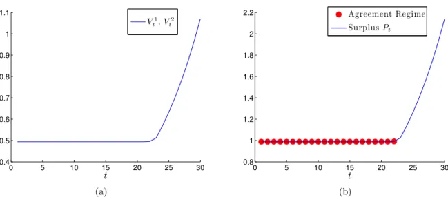
2.1 A Symmetric Model with MPE E0 Played at Date T . . . 61
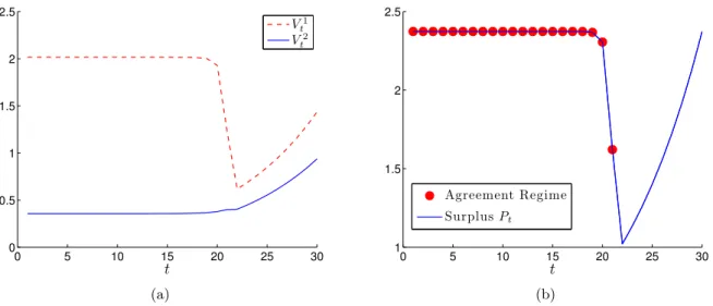
2.2 An Asymmetric Model with MPE E1 Played at Date T . . . 63
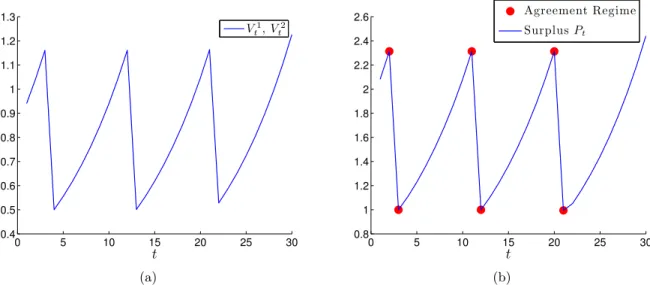
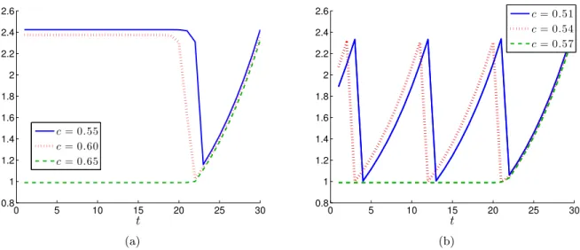
2.3 Cycling Between Agreement and Disagreement Regimes . . . 65
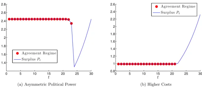
2.4 No Cycling with Asymmetric Political Power or High Costs . . . 66
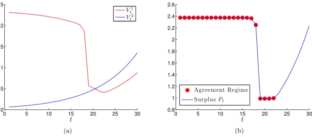
2.5 A Shift in Political Power . . . 67
1 Political Business Cycles with Policy Compromise
1.1 Introduction
The literature on political business cycles argues that the election cycle affects policy outcomes. This hypothesis is based on the idea that once political considerations, such as a party’s desire to be in power or to implement policies that are consistent with its views, are taken into account, elections influence policy decisions. Empirical analysis supports the notion that there is a relationship between the election cycle and fluctuations in policy variables, citing evidence of cycles in government budget deficits (Alesina, Cohen, and Roubini, 1992; Shi and Svensson, 2006), tax policy (Persson and Tabellini, 2003), and economic growth (Drazen, 2000).
In representative democracies where policy decisions are made by a legislature, negotiations amongst political parties determine policy outcomes and the nature of political business cycles. When considering legislative policy-making, the policies that emerge are not only a function of the observable actions that parties take (e.g., attending legislative hearings, writing legislation, or voting on a proposed bill), but also the result of parties’ actions that are unobservable or “hidden.” For instance, often in legislatures such as the United States Congress, private strategy sessions amongst the members of a party occur multiple times a week. A specific example of these meetings are the party lunches amongst members of the US Senate that often occur Tuesday, Wednesday and Thursday of each week. Similarly, in the UK Parliament or the US Congress, the party leadership, such as the whip, will have private conversations with members of the party to encourage certain voting behavior or attendance at important policy debates. These private meetings amongst the members of a party often shape the party’s stance on particular issues, and hence, influence the policy outcomes that result from negotiations between political parties.
cooperation, with efforts at bipartisanship, inefficient political cycles can emerge.
The existing literature that focuses on how negotiations between political parties produce political cycles (Alesina, 1987) or policy distortions (Acemoglu, Golosov, and Tsyvinski, 2010) demonstrates that in constrained efficient equilibria, political cycles or distortions are largely insignificant if parties’ actions are observable and parties place a high value on future policy outcomes (i.e., parties have high discount factors). My paper therefore complements this literature by showing that, in an environment where parties take hidden actions that influence policy outcomes, even when parties are arbitrarily patient and coordinate on a constrained surplus-maximizing equilibrium, inefficient political cycles can emerge. Thus, with patient parties, political cycles are not only consistent with the notion of myopic political parties that choose policies that are only optimal from a short-run perspective. Indeed, political cycles can even be generated by strategies that aim to maximize expected welfare.
I model government policy-making as an infinite-horizon game played by two political parties. Each period, one party is “in power,” where the evolution of political power is taken as given and political power may change hands every other period. At the beginning of each period, the party in power determines how the government budget should be allocated between two public projects, where each party has a preferred project and receives no payoff from spending on the other’s preferred project. In the same period, after this allocation decision has been made, parties simultaneously choose an action (“investment effort”) that stochastically affects economic growth, where higher growth means, in expectation, a larger government budget in the future. This action choice has two key features. One, each party’s choice is unobservable to the other party. Two, when making this choice, a party faces a tradeoff between securing itself a high benefit today or generating a large government budget tomorrow. Given any pair of investment efforts, there is a common expectation amongst parties regarding the expected size of tomorrow’s budget. The identity of the party in power, the size of the government budget, and the allocation of that budget are all commonly known.
in any surplus-maximizing policy, there are no cyclical fluctuations in the size of the budget or in parties’ investment efforts. Political cycles are therefore necessarily inefficient in the model. Inefficient political cycles surface in constrained surplus-maximizing equilibria as the un-observable effort choice creates a moral hazard problem (the game is one of imperfect public monitoring). As parties’ efforts today stochastically determine the size of the budget tomor-row, if a party observes a small government budget at the beginning of the period, it cannot be sure if this is due to a bad shock to the economy or to the other party focusing its efforts not on future growth, but on its own interests.1 The nature of cooperation, whether in the form
of parties sacrificing current partisan objectives for the sake of budget growth or through the party in power implementing more equitable divisions of the budget, is affected by the severity of this moral hazard problem. This is best illustrated by considering a variant of the model where the investment effort is observable. If parties are sufficiently patient, it is possible to construct an equilibrium that sustains the surplus-maximizing policy. In this equilibrium, by simply threatening to revert to a “bad” equilibrium with low payoffs in the event that a party deviates to a non surplus-maximizing effort choice. In contrast, when effort is unobservable, such a strategy will no longer work as it is not possible to observe when deviations have oc-curred. Cooperation on “good” policies each period is therefore more difficult to sustain and inefficient policy outcomes, and hence political cycles, can arise.
The main result of the paper establishes that, if parties’ efforts toward cooperation are com-plimentary, constrained surplus-maximizing equilibria display political cycles. These strategies are based on the idea that nontrivial intertemportal incentives can be used to enforce certain effort levels, where parties are “punished” or “rewarded” based on whatever information is publicly available about parties’ past effort choices. In my model, this implies that the future payoffs (the punishments and rewards) that parties receive must be conditioned on the size of the government budget that is realized at the beginning of a period. Consider a constrained surplus-maximizing equilibrium where both parties must choose to exert high effort in order
1Note that if the pair of investment choices today determined, with probability one, the size of the budget
to maximize aggregate surplus. In order to provide parties with an incentive to put aside partisan differences and choose high effort levels, the equilibrium must use strategies where “bad”, or low, realizations of the budget trigger a reversion to a punishment phase where both parties receive a low payoff. In this punishment phase, the size of the government bud-get is, in expectation, inefficiently low. Furthermore, the budbud-get can exhibit high frequency cyclical fluctuations where the budget is, in expectation, smaller immediately after an elec-tion, compared to the budget in the middle of the term. Hence, it is possible for constrained surplus-maximizing equilibria to exhibit political cycles.
I now discuss some features of my approach. In the model, political parties cannot make any binding commitments to either future allocations or investment efforts. Hence, the only constraint on policies at any date is that they are consistent with parties acting rationally given the current state of the environment (i.e., the date, which party is in power, and the size of the budget) and any information about past play. Regarding the notion of a political party, though parties disagree on how to allocate the budget, they share a common view regarding what generates budget growth. If one considers a party as a group from the same geographically-defined district, the model is consistent with the idea that parties compete to secure funding for local public goods (e.g., local infrastructure and parks), but agree on what types of investments stimulate budget growth. Alternatively, one can consider parties with ideological differences that compete to secure funding for “pet projects” (e.g., farm subsidies, museums, local public goods), and while they may disagree in general on what investments stimulate growth, there is agreement on a subset of investment policies (e.g., tax reform and education) that foster growth.
spending or on legislation that invests in national infrastructure, where this investment in-creases productivity, and thus the pool of taxable income. Likewise, a party can work towards passing legislation that includes tax breaks and subsidies for the group it represents, or on tax code reform that generates higher government revenues directly, or indirectly by increasing productivity, and hence increasing the national tax base. Second, the assumption that each party’s effort choice is unobservable to the other party is consistent with the ideas discussed earlier. Policy outcomes, and specifically budget growth, are often influenced by the unob-servable actions that parties take during the policy-making process, whether during the whip process, in small committee meetings or in partisan strategy sessions. If parties are unwilling to engage in the bipartisan cooperation that is required for “good” policies, then wasteful programs will persist and budget-growing policies, such as a tax code free of loopholes and credits, will fail to be implemented.
The remainder of the paper is structured as follows. Section 2 reviews the related literature in greater detail. The model is introduced in Section 3. Section 4 considers surplus-maximizing policies and constrained surplus-maximizing equilibria under perfect monitoring. Section 5 considers constrained surplus-maximizing equilibria under imperfect public monitoring. Fi-nally, Section 6 concludes. The Appendix contains omitted proofs.
1.2 Related Literature
Broadly speaking, there have been two types of theories that aim to rationalize political busi-ness cycles: a theory that focuses on politicians’ “opportunistic manipulation” of voters and a “partisan” theory that considers how differences in political parties’ policy preferences pro-duce cycles. I now review each strand of literature in turn. Before doing so, it is important to note that in all of the papers mentioned below, Pareto efficient policies do not exhibit cyclical dynamics; hence, if the political economy friction that is introduced causes political cycles, these cycles are inefficient.
heavily influence voters’ decisions.2 Politicians will then, to the best of their ability, influence
the economy or other policy variables in an effort to be reelected. This is the basic observation that motivates the literature on opportunistic manipulation.
One of the first models of opportunistic political cycles, developed by Nordhaus (1975), considers an economy that is represented by a downward-sloping Phillips curve with (homoge-nous) voters with (irrational) adaptive expectations. Given that voters prefer low inflation and low unemployment, the office-seeking politician can secure reelection by depressing the econ-omy for most of her term until right before the election, where the econecon-omy is stimulated with expansionary monetary policy. The economy then follows a cyclical pattern with expansionary policy right before the election and contractionary policy right after the election.
In an effort to model opportunistic political cycles with fully rational voters, Rogoff (1990), along with much of the subsequent literature focusing on opportunistic manipulation, considers a model based on an informational asymmetry between voters and the politician. More specif-ically, Rogoff supposes that politicians differ in their competence, where highly competent politicians can provide more public goods at a lower level of taxes. Moreover, an information structure is assumed where (homogenous) voters are uninformed about one element of fiscal policy but can perfectly monitor the politician with a one-period lag. In the first half of the term policy is efficient, while in the second half of the term a competent politician sets taxes too low and spending too high in order to communicate her ability. Hence, a political business cycle may be generated due to a politician attempting to signal her private information.
Other papers of opportunistic manipulation based on signaling include Shi and Svensson (2006), Martinez (2009), and Drazen and Eslava (2006). Shi and Svensson (2006) consider a model similar to Rogoff’s, and find that the size of a pre-election spending boom, and hence the political cycle, depends positively on the portion of “uninformed” voters and the ego-rent collected by the politician.3 While Rogoff and Shi and Svensson assume an information
structure where voters are only uninformed at the end of the term—thus limiting the role
2See, for instance, Drazen (2000) and the references therein. 3
of signaling to this time period—Martinez (2009) considers a political-agency model where voters are imperfectly informed at all times and is able to show that politicians may have a greater incentive to generate “good” economic conditions near the end of the term. In contrast to these papers, Drazen and Eslava (2006) consider a model of voter manipulation with heterogeneous voters that can view all aspects of fiscal policy and politicians that are all equally “competent.” Voters are differentiated based on the types of government spending they prefer and a politician has private information regarding her preferences over spending. They show that there exists an equilibrium where there is a political cycle in the composition of the budget, with higher targeted spending for the group of voters that is more likely to swing the election.
Now, I consider papers on the partisan theory, where these models focus on how negotia-tions amongst political parties with different policy preferences generate political cycles. Hibbs (1977) presents one of the first partisan models. As in Nordhaus’s model, the economy is rep-resented by a downward-sloping Phillips curve and voters do not have rational expectations.4
Two political parties have different preferences over inflation and unemployment, and due to irrational expectations, the party in power can cause inflationary surprises. This implies that cycles then arise in the economy, with fluctuations coming due to changes in which party is in power.
Towards developing a partisan theory with fully rational agents, Alesina (1987) develops a partisan model that focuses on cycles in macroeconomic outcomes, but allows for voters to have rational expectations. In such a model, only unanticipated monetary policy can affect real variables. Policy-making is modeled as a dynamic game of perfect information, where the party currently in power chooses policy. The uncertainty caused by the election, coupled with an assumption on the rigidity of nominal wage contracts, implies that there will be surprise inflation at the beginning of a party’s term in power. There will then be the following cycle: in the first part of the term, under the left-wing party policies will be relatively expansionary while under the right-wing party policies will be relatively contractionary; in the second part
of the term parties implement the same policy.
are sufficiently patient (as I assume in my paper), in constrained surplus-maximizing equilib-ria, policy distortions—and hence, political cycles—will vanish. Policy distortions (and any associated political cycles) are therefore on the equilibrium path when considering inefficient equilibria (i.e., equilibria that are not constrained efficient) or constrained surplus-maximizing equilibria in a model where parties are impatient. In contrast, in my paper even when parties are patient and play a constrained surplus-maximizing equilibrium, political cycles can arise and are persistent.
1.3 The Model
Time is discrete and indexed by t ∈ {1,2, . . .}. Let N = {1,2} denotes the set of parties.
At each date, exactly one party is the party in power. Political power potentially changes hands at the beginning of every odd period, where the evolution of political power follows an exogenously given, time invariant, irreducible Markov process. For any period 2z, where z∈ {1,2, . . .}, with partyk∈N currently in power, let m(i|k)∈(0,1) denote the probability that partyiis in power at the beginning of the next period.
At the beginning of each period t, there is income yt∈Y ={0, y}, wherey >0. I assume there is zero income at the beginning of period 1. In periodt, the party in power determines the allocation of the incomeyt, denotedct, wherect∈C(yt) ={c1
t, c2t ∈[0, yt]2:c1t+c2t ≤yt}. After the income yt has been allocated, parties simultaneously choose actions, where party i∈N chooses an actionai∈Ai = [0,1].
The action profile a∈ A =A1×A2 affects r and π, where r is a payoff vector and π is
the probability distribution that stochastically determines the income level at the beginning of the next period. Specifically, given the action profilea∈ A, partyi gets a payoff of ri(ai) and the probability of obtaining the high income realization ofy isπ(a), while the probability of obtaining the low income realization of 0 is 1−π(a).
Timet Time t+ 1
Iftis odd,
power may shift Incomerealizedy chooses allocationParty in Power c∈C(y)
Parties choose a
Figure 1.1: Timeline of Period t
The following assumptions on the payoff functionrand the probabilityπare made through-out the entire paper.
Assumption 1 Given i∈N,ri(ai) =−ai for any ai ∈Ai, andπ(·, a−i) is increasing in ai for any a−i ∈A−i.
Thus, higher actions give each party i a lower immediate payoff r, but generate higher expected income in the future. Each party then faces a tradeoff when choosing an action: lower actions generate a higher payoff today, while higher actions generate a higher expected return tomorrow.
Assumption 2 π is concave, differentiable and satisfies the following Inada conditions
lim ai→0
∂π(a1, a2)
∂ai =∞ and limai→1
∂π(a1, a2)
∂ai = 0 ∀a
j ∈[0,1]
1.3.1 An Imperfect Monitoring Game
In what follows, I consider a stochastic game of imperfect public monitoring (see, for instance, Fudenberg and Yamamoto, 2011, and H¨orner et al, 2011). Specifically, for any periodt, while the party in power kt∈N, the income realization yt∈Y, and the allocation decisionc∈R2
are public information, the actionai∈Aitaken in any periodtis private information for party i∈N. The upcoming analysis also applies to the case where the action profilea∈A for any periodtis public information, with comparisons to this case being made occasionally below.
The public history at the beginning of period tis
ht= (k1, y1,(c11, c21), . . . , kt−1, yt−1,(c1t−1, c2t−1), kt, yt).
The set of public histories at the beginning of periodtis thenHt= (N×Y ×R2)t−1×(N×Y)
and H=∪t≥1Ht denotes the set of all public histories. The private history for party iat the
beginning in periodtis a sequence
hit= (k1, y1,(c11, c21), ai1, . . . , kt−1, yt−1,(c1t−1, ct2−1), ait−1, kt, yt).
The set of private histories at the beginning of period t is then Hi
t =HtS(Ai)t−1 and Hi =
∪t≥1Hti denotes the set of all private histories.
A (behavior) strategy for partyiis given byσi ={γi, ωi}, whereγi :Hi→ ∪
y∈Y ∆(C(y)) and ωi :Hi →Ai. As parties utility is linear in consumption and π is concave, it is without loss of generality to limit attention to the set of pure actionsAi for each i∈N. Parties seek to maximize the average discounted sum of their expected flow payoffs, where given the initial party in power k1, initial income y1, and strategy profileσ, this payoff is
∞ X
t=1
(1−δ)δt−1Ek1,y1,σ[−a i t+cit].
of public strategies such that, for any period t and public history ht, σ|ht (the continuation
strategy induced byht) is a Nash equilibrium from that period on. Note that the set of PPE is a subset of the set of sequential equilibria.
1.4 Surplus-Maximizing Policies and Perfect Information
Before considering the (constrained) surplus-maximizing PPE of the imperfect monitoring game, it is useful to consider both the surplus-maximizing polices and the (constrained) surplus-maximizing equilibrium with perfect monitoring.
1.4.1 Surplus-Maximizing Policies
Given any states0 ∈S, the set of surplus-maximizing policies are characterized by considering
the following problem
max
{at,ct}∞t=1
Ek1,y1
∞ X
t=1
(1−δ)δt−1
−a1t +c1t+−a2t +c2t
,
whereat∈Aand ct∈C(yt). As this problem is stationary and parties’ utility from income is linear, the action profile in any surplus-maximizing policy is time-invariant, i.e.,a∗t =a∗t0 ≡a∗
for any periods tand t0. The action profile a∗ is found by considering the action profile that maximizes expected surplus over two periods. Formally,a∗ is the solution the problem
max a∈[0,1]2 −a
1−a2+δπ(a)y.
Given that π is concave and differentiable, as π is assumed to satisfy the Inada conditions outlined in Assumption 2, the solution to this problem is characterized by the optimality condition
−1 +δ∂π(a)
∂ai y = 0 ∀i∈N. Thus, in each periodt,ai
t=ai∗ whereai∗ satisfies the above optimality condition. As parties’ utility from income is linear, in any period t, in the event of a high income realization, any allocationctsuch thatc1
government budget is identical, in expectation, entering any period in any surplus-maximizing policy. Hence, there are no political cycles in any surplus-maximizing policy.
1.4.2 (Constrained) Surplus-Maximizing Equilibria Under Perfect
Informa-tion
The following lemma establishes that, if parties are sufficiently patient and monitoring is perfect, it is possible to construct an equilibrium that delivers the highest possible social surplus of−a1∗−a2∗+δπ(a∗)y.
Lemma 1. Suppose monitoring is perfect. There exists a δ¯∈ (0,1) such that for any δ ≥δ¯ there is an equilibrium that sustains a surplus-maximizing policy.
Proof. See the Appendix.
1.5 (Constrained) Surplus-Maximizing PPE Under Imperfect Monitoring
In this section, I consider (constrained) surplus-maximizing PPE and, more specifically, the equilibria when parties are sufficiently patient. As illustrated in the previous section, if moni-toring is perfect and if parties are sufficiently patient, it is possible to construct an equilibrium that delivers the highest possible surplus. In contrast, with imperfect public monitoring, this is not possible. The following lemma establishes that, regardless of how patient parties are, the surplus from any (constrained) surplus-maximizing equilibrium is necessarily less than the highest possible surplus.
Lemma 2. Given anyδ ∈(0,1), the surplus from any (constrained) surplus-maximizing PPE is strictly less than the surplus from any surplus-maximizing policy.
Proof. See the Appendix.
punishment?
The main result, Proposition 1, establishes that if parties efforts are complementary (in the sense described in Assumption 3 below), then as parties become sufficiently patient, it is always possible to construct an equilibrium with high initial efforts and a punishment phase, that improves on any “no punishment” equilibrium. Hence, surplus-maximizing equilibria require a punishment phase, and thus, as I will discuss shortly, political cycles.
I use the following assumption for some of the results stated in the rest of the paper.
Assumption 3 Supposeai> aj. Thenπ(ai, aj)< π(ai−ε, aj+ε),whereε∈(0,min{ai, ai− aj}).
Assumption 3 implies that the probability π is symmetric and that parties efforts towards cooperation are complements. The following lemma characterizes the benchmark equilibrium discussed above that does not use punishments.
Lemma 3. Under Assumption 3,
1. There exists a δ¯∈(0,1) such that for any δ ≥δ¯, there is an equilibrium where, in each period t, each partyi∈N chooses an actionai
t where
−1 +δ∂π(at) ∂ai
t y 2 = 0;
2. This equilibrium generates the highest surplus amongst all equilibria that do not use punishments.
Proof. See the Appendix.
expected surplus from the continuation payoffs in the event of a high income realization is strictly greater than the surplus in the event of a low income realization. In the main result, Proposition 1, I show that, ifδ is sufficiently large, then any (constrained) surplus-maximizing equilibrium requires these higher actions initially.
Notation and Preliminaries. The following notation and terminology is used is some of
the results in the remainder of the paper. It is useful to introduce the following state space
S. Let T ={t1, t2} and S =N ×T, where s∈S specifies the identity of the party in power
and whether it is the first part of the term (datet1 ) or the second part of the term (datet2).
Given a state s0 ∈ S at the beginning of the period, let p(s|s0) denote the probability that state is s∈S at the beginning of the next period, where
• Given (j, t1)∈S,p(j, t2|j, t1) = 1;
• Given (j, t2)∈S,p(i, t1|j, t2) =m(i|j) for any j∈N.
Define party i’s minmax payoff for initial state s, initial income 0 and discount factorδ
vis= min σ−i maxσi
∞ X
t=1
(1−δ)δt−1Es,σ[−ait+cit].
Asδ →1,vi
sconverges to partyi’s limit-average minmax payoff with initial statesand income 0. (see Mertens and Neyman, 1981). As the Markov chain overS is irreducible, as δ→ 1,vi
s is independent of the initial states(see, for instance, Dutta 1995).
Before stating Proposition 1, the following lemma characterizes the “worst” equilibrium for each party i∈N, where in the worst equilibrium for party i, partyi receives its minmax payoff. These equilibria (or equilibrium if there is one equilibrium that gives each party its minmax payoff) are used when constructing an equilibrium that gives higher surplus than any “no punishment” equilibrium.
Lemma 4. Given an initial states∈S, there exists a ¯δ∈(0,1)such that for any δ ≥δ¯there is an equilibrium with the payoff vector ˆvs such that ˆvi
Proof. See the Appendix.
The equilibrium constructed in Lemma 4 features a temporary phase of mutual minmaxing, followed by a return to an equilibrium that gives each partyia payoff strictly higher then the payoff ˆvi
s. The behavior during the phase of mutual minmaxing can be described as follows. The party in power takes all the income at the beginning of each period. In the first part of the term, the party out of power j chooses the lowest possible actionaj = 0, while the party in power ichooses the action that solves
max ai∈[0,1] −a
i+δπ(ai,0)y.
In the second part of the term, both parties chooses the lowest possible action 0. Hence, there are high frequency cyclical fluctuations during the phase of mutual minmaxing, as the size of the government budget is, in expectation, smaller at the beginning of the first part of the term than at the beginning of the second part of the term.
The statement of Proposition 1 relies on the following strategy. Consider Strategy SM:
• There are the following eight phases: Phases (As) and Phases (Bs). Transitions between phases may only occur after the party-in-power’s allocation decision in a particular pe-riod. Given an initial states∈S at date 1, begin in PhaseAs.
• Given an initial state s∈S, in Phase As, the action profile a∗ is played. If in PhaseAs and there is a positive income realization, each party receivesy/2.
• If in Phase As0 and there is a high income realization, if the next state is s, move to
Phase As. If in Phase As0 and there is a low income realization, if the next state is s,
with probabilityρs∈(0,1) move to Phase As and with probability 1−ρs transition to PhaseBs.
• If currently in Phase Bs and the previous phase was Phase As0, with probability ξs
• If currently in Phase As and there is a positive income realization, if the consumption allocation cs 6= (y/2, y/2), revert to the worst equilibrium for the party currently in power.
Proposition 1. Under Assumption 3, there exists a ¯δ ∈ (0,1) such that for any δ ≥ δ¯, Strategy SM is an equilibrium that generates higher expected surplus than any “no punishment” equilibrium.
Proof. See the Appendix.
The intuition for the proof of Proposition 1 is as follows. The strategy featured in Proposi-tion 1 (Strategy SM) begins with parties choosing an acProposi-tion profile that yields a higher social surplus than the action profile in the benchmark equilibrium constructed in Lemma 3. If δ is sufficiently large, then the transition probabilities (ρs) required for the action profile a∗ to be incentive compatible get close to 1. Thus, the probability of transitioning to the punish-ment phase becomes sufficiently small so that an equilibrium generates higher surplus than the equilibrium constructed in Lemma 3 that does not rely on punishments.
It is important to note that without Assumption 3, the problem of characterizing (con-strained) surplus-maximizing equilibria is less tractable. Essentially, if parties’ efforts towards cooperation are not complementary and symmetric, it may be too costly to provide incentives for both parties to choose high actions initially. Indeed, this may not be consistent with a (constrained) surplus-maximizing equilibrium. Characterizing these equilibria then involves comparing different “punishment” and “no punishment” equilibria, where it is not straightfor-ward to determine which yield a greater expected surplus.
periods where the (expected) size of the budget is low. Furthermore, during a stretch of bad policy where parties are minmaxing each other, recalling the worst equilibrium constructed in Lemma 4, the equilibrium can display high frequency political cycles. In these political cycles the (expected) size of the government budget is smaller at the beginning of the first part of the term as compared to at the beginning of the second part of the term.
1.6 Conclusion
This paper analyzes a model of government policy-making where political business cycles arise due to parties’ hidden actions, fluctuations in political power and differences in parties’ views over the optimal allocation of the government budget. I suppose political parties have a high discount factor and consider the set of constrained surplus-maximizing equilibria, where the assumption that each party’s investment effort choice is unobservable generates a moral hazard problem that has key implications on how close the payoffs from these equilibria are to the Pareto frontier. Equilibrium payoffs are bounded away from the Pareto frontier. When PPE payoffs are necessarily inefficient, if efforts toward bipartisanship are complementary, constrained surplus-maximizing equilibria have cyclical dynamics. Hence, there are inefficient political cycles on the equilibrium path.
1.7 Appendix
1.7.1 Characterization of Minmax payoffs
The strategy profile that party j uses to minimize the other party i’s payoff is described as follows.
• When out of power, j choosesaj = 0.
• When in power, in the first part of the term, partyj chooses any actionaj ∈[0,1] and takes all the income that is realized at the beginning of the period.
• When in power, in the second part of the term, party j choosesaj = 0.
First, when in power, party j minimizes party i’s payoff by giving j none of any income that is realized at the beginning of the period. In regards to party j’s action choice in the first part of the term, asj will be in power in the next period, and thus can ensure thatiwill receive an expected payoff of zero (regardless of what action profile is played in the first part of the term), any actionaj ∈[0,1] is consistent withj minmaxing i. When j is in power and it is the second part of the term, or ifj is not in power,j minimizesi’s payoff by choosing the lowest possible effortaj = 0.
In response to this strategy, party iwill find the following optimal
• When out of power, in the first part of the term, ichoosesai= 0.
• When out of power, in the second part of the term, isolves
max ai∈[0,1] −a
i+δπ(0, ai)m(i|j)y.
• When in power, in the first part of term, take all the realized income and solve
max ai∈[0,1] −a
• When in power, in the second part of term, take all the realized income and solve
max ai∈[0,1] −a
i+δπ(0, ai)m(i|i)y.
Given the strategy j uses to minimize i’s payoff, when out of power, in the first part of the term, i knows that it will receive non of the income in the next period; hence, ai = 0 is optimal. When out of power, in the second part of the term, considering that aj = 0 and the probability of gaining power (and hence getting all the income) is m(j|i), party isolves the problem outlined above. Similarly, when in power, in the second part of the term, considering thataj = 0 and the probability of gaining power (and hence getting all the income) ism(i|i), party i solves the problem outlined above. Finally, when in power, in the first part of the term, considering that aj = 0 and the probability of gaining power (and hence getting all the income) is 1, party i chooses the action outlined above. This strategy will yield the minmax payoff vector.
1.7.2 Omitted Proofs
Proof of Lemma 1
Leta∗denote the action profile that maximizes social surplus. Consider the following strategy: • Begin in Phase A.
• If in Phase A, the action profilea∗ is played and each party receivesy/2 in the event of a positive income realization.
• Ifai
t6=ai∗ or ifct6= (y/2, y/2), with the party in poweri, revert to the worst equilibrium for party i; otherwise, remain in Phase A.
Define the payoff vector v as follows
vis∗0 =−(1−δ)ai∗+δ X
s∈S
p(s|s0)hπ(a∗)(1−δ)y 2 +vi
∗
s
In order for the action ai∗ to be consistent with equilibrium, given the state s0 ∈ S, the
following constraint must be satisfied
vi∗
s0 ≥ −(1−δ)ai+δ X
s∈S
p(s|s0)hπ(ai, aj∗)(1−δ)˜ci s+vis
+ (1−π(a∗)vi s
i
for eachi∈N, anyai 6=ai∗ and ˜ci
s=y ifi is the party in power and ˜cis = 0 is not the party in power. Also, the allocation constraint for the party in power i
(1−δ)y
2 +vsi∗ ≥(1−δ)y+vis. As surplus under this strategy is maximized and, as δ → 1, v1
s → v2s for any s ∈ S, if δ is large enough, both the incentive constraint for actions and the party-in-power’s allocation constrained are satisfied in each periodt. Hence, there exists an equilibrium with payoff vector vs∗ in stateswhere v1∗
s +v2s∗=−a1∗−a2∗+δπ(a∗)y.
Proof of Lemma 2
By contradiction. Suppose that the surplus-maximizing action profile a∗ can be supported in
each period. Then there exists continuations (ws(0), ws(y)) and allocations (cs) such that
ai∗ = arg max
ai∈[0,1] −(1−δ)a
i+δX
s∈S
p(s|s0)hπ(a∗)(1−δ)csi +wis(y)+ (1−π(a∗))wis(0)
This implies the following optimality conditions for i’s action
(1−δ) =δX s∈S
p(s|s0)∂π(a
∗)
∂ai
h
(1−δ)cis+wsi(y)−wis(0)i.
Noting that
δ∂π(a
∗)
and summing the two optimality conditions, we have
2(1−δ) = 1 y
X
s∈S
p(s|s0)h(1−δ)y+w1
s(y) +w2s(y)−(w1s(0) +w2s(0)
i
.
If a PPE existed that gave the same surplus as the surplus-maximizing policy, then w1
s(y) + w2
s(y) =ws1(0) +ws2(0). Considering the condition immediately above, this implies 2(1−δ) = (1−δ)
giving the contradiction.
Proof of Lemma 3
Part 1. Given the initial state s0 ∈ S, if party i finds it optimal to choose the ai in the statement of the Lemma, then
−(1−δ) +δ∂π(a) ∂ai
X
s∈S
p(s|s0)h(1−δ)csi +wsi(y)−wis(0)i= 0
where, as ∂π(a)
∂ai = yδ2,
X
s∈S
p(s|s0)h(1−δ)cis+wis(y)−wsi(0)i= (1−δ)y 2
for each i∈N.
Note that the payoff vector vs0 satisfies the following for eachi∈N
vis0 =−(1−δ)ai+δ X
s∈S
p(s|s0)π(a)h(1−δ)cis+wsi(y)−wis(0)i+δX s∈S
p(s|s0)wsi(0);
hence, using the equality immediately above, we have
vsi0 = (1−δ) h
−ai+π(a)y 2
i
+δX s∈S
As each perioda1 =a2 and each party ireceives the flow payoff−ai+π(a)y
2, it must be the
case that the equilibrium payoff, regardless of the income realization at the beginning of the period, is
vsi0 =−ai+δπ(a)
y
2 ∀s0 ∈S, i∈N. This implies thatci
s =y/2 for anys∈S, i∈N.
In order to guarantee that this is an equilibrium, the allocation constraint for the party in power i needs to be checked. With vi
s =vi for each s ∈S, given an initial state s∈ S, this allocation constraint is
(1−δ)y
2 +vi ≥(1−δ)y+vis.
First, note that, under Assumption 3, the surplus from the strategy outlined in Lemma 3 yields an expected surplus that is strictly greater than the surplus v1
s+v2s for any s ∈S. Second, v1=v2 and v1
s→v2s for any s∈S asδ →1. These two pieces imply that if δ is large enough then the allocation constraint is satisfied for any Markov process that satisfies the assumptions outlined in The Model presented in Section 3. Hence, the strategy proposed in Lemma 3 is an equilibrium for δ large enough.
Part 2. It remains to show that this equilibrium generates the highest expected surplus
amongst all equilibria that do not use punishments. The argument makes use of the following lemma.
Lemma 5. Under Assumption 3, there exists a δ¯ ∈ (0,1) such that for any δ ≥ δ¯, in any constrained surplus-maximizing equilibrium both parties choose the same action in the first period.
Proof. By contradiction. Fix a constrained surplus-maximizing equilibrium σ. Given the initial state s0, suppose a is the action profile in the current period, wherea1 6=a2, c
receives all the income in the event of a positive income realization, there is an alternative equilibrium that delivers the same payoff and gives both parties positive consumption. With this in mind, suppose ci
s∈(0, y) for each i∈N.
Without loss of generality, suppose a1 > a2. Consider the strategy ˆσ, with the action
profile ˆa, with ˆa1=a1−εand ˆa2=a2+ε, where ε >0 is very small. The consumption profile
(ˆcs) will be defined below and the continuations {wˆs(0),wˆs(y)} are such that ˆws(0) = ws(0) and ˆws(y) =ws(y) for each states∈S.
Given the actions (ˆa1,aˆ2), for eachs, I now show that there exists a consumption allocation
ˆ
cs such that
−ˆai+δπ(ˆa)ˆcsi ≥ −ai+δπ(a)cis
for eachi∈N. First, there exists a ¯ε >0 such that for anyε∈(0,ε¯), there exists a ˆc1
s ∈(0, y) where
−a1+δπ(a)c1s=−aˆ1+δπ(ˆa)ˆc1s. Choose ε∈(0,ε¯) and such a ˆc1
s. Noting that
−ˆa2+δπ(ˆa)ˆc2s =−ˆa2+δπ(ˆa)(y−ˆc1s)
we have
−ˆa2+δπ(ˆa)ˆc2s =−ˆa2+δπ(ˆa)y+ε−δπ(a)c1s
>−a2+δπ(a)(y−c1s) (by Assumption 3) =−a2+δπ(a)c2s,
and we have established, under the action profile ˆa, there is a Pareto improvement. It remains to show that the consumption allocation ˆcs is incentive compatible for the party in power for each s ∈ S. Noting that the allocation cs is incentive compatible and that ci
incentive compatible. Hence, if δ is sufficiently large, there exists an alternative equilibrium ˆ
σ that Pareto dominates σ. A repeated application of this argument establishes the desired result.
Fix δ ∈ (0,1) such that, under Assumption 3, in any constrained surplus-maximizing equilibrium parties choose the same action profile. Towards a contradiction, suppose there exists an equilibrium that does not use punishments with an action profilea0 6=a, where ais the action profile characterized in Part 1. The optimality condition for this action choice for party iis
−(1−δ) +δ∂π(a) ∂ai
X
s∈S
p(s|s0)h(1−δ)cis+wsi(y)−wis(0)i= 0.
Asa1=a2, under Assumption 3, adding these two optimality conditions and noting that
X
s∈S
p(s|s0)hws1(y) +w2s(y)i=X s∈S
p(s|s0)hws1(0) +w2s(0)i,
we obtain
δ∂π(a)
∂ai (1−δ)y= 2(1−δ). This implies that ∂π(a)
∂ai = yδ2 for eachi∈N. Hence, parties choose the same action as outlined in Part 1 and a contradiction is obtained. Therefore, for δ sufficiently large, the equilibrium constructed in Part 1 offers the highest expected surplus amongst all equilibria that do not use punishments.
Proof of Lemma 4
The proof of Lemma 5 relies on the following lemma.
Lemma 6. Given δ ∈(0,1) and s∈S, there exists an equilibrium with payoff vector v such thatvi
s > vis for anyi∈N.
Proof. Consider the following equilibrium
• In any period, the party in power receives all the income in the event of a positive
• If partyj is out of power and it is the first part of the term, partyichooses aj = 0.
• If partyi is in power and it is the first part of the term, party ichooses an action that solves
max ai∈[0,1] −a
i+δπ(ai,0)y.
• If partyiis out of power and it is the second part of the term, partyichooses an action that solves
max aj∈[0,1] −a
j+δπ(ai, aj)m(j |i)y.
• If partyiis out of power and it is the second part of the term, partyichooses an action that solves
max ai∈[0,1] −a
i+δπ(ai, aj)m(i|i)y.
Notice that the expected payoff that each party receives from the action choice in the first part of each term is the same as the strategy that implements the minmax payoff profile. On the other hand, the expected payoff that each party receives from the action choice in the second part of the term is strictly greater than that received from the strategy that implements the minmax payoff profile. Hence, under this equilibrium each party receives an expected discounted payoff that is strictly greater than its minmax payoff.
Now for the proof of Lemma 5. Consider the following strategy, denotedσi, that generates the payoff vector v
s withv i s=v
i s.
• There are two phases: Phases A and B. Play starts in Phase A. In Phase B, the
equilib-rium constructed in Lemma 6 is played.
• In Phase A, the party in power receives all income in the event of a positive realization.
In the first part of the term, the party out of powerj chooses aj = 0, while the party in power chooses an action that solves
max ai∈[0,1] −a
In the second part of the term, each partyi∈N choosesai = 0.
• If there is a low income realization in the second part of the term, with probability ρs play shifts to Phase B while with probability 1−ρs play remains in Phase A. If there is a high income realization in the second part of the term, play remains in Phase A. In the first part of the term, regardless of the income realization, play remains in Phase A.
First, let ˆvs denote the payoff vector for the equilibrium constructed in Lemma 6. Second, note that there always exists (ρs), whereρs∈(0,1) for each s∈S, such that the strategy σi generates exactly the payoffvi
s. Third, consider the action and allocation incentive constraints. As the party in power simply takes all the income in the event of a positive realization, the allocation constraint is always satisfied. In the first part of the term, as continuations are independent of the income realization, the prescribed action profile is incentive compatible. In the second part of the term, as each party’s payoff ˆvi
s from the equilibrium in Lemma 6, is strictly greater than the payoff vectorvi
s for any i∈N, ifδ is large enough, (1−δ)cis+ρs(ˆvsi−vis)<0
for each i ∈ N. Hence, party i’s is decreasing in ai and ai = 0 for each i ∈ N is incentive compatible. It follows that the proposed strategy is an equilibrium and, thus, there exists an equilibrium that delivers the minmax payoffvi
s ifδ is sufficiently large.
1.7.3 Proof of Proposition 1
Let ¯δ be such that for any δ ≥ ¯δ, any constrained surplus-maximizing equilibria has both parties choosing the same action in the first period. ConsiderStrategy SM, where the surplus-maximizing profile a∗ is played in the first period. The payoff vector v
s0 from this strategy is
defined by
vsi0 =−(1−δ)ai∗+δπ(a∗) X
s∈S
p(s|s0)h(1−δ)cis+(1−ρs)(vsi−vˆis)i+δX s∈S
where (ˆvs) is the payoff vector from the equilibrium outlined in Strategy SM where with probabilityξsthe worst equilibrium for party 1 and with probability 1−ξsthe worst equilibrium for party 2. Note that there always exists a ξs∈(0,1) such that ˆv1
s = ˆvs2.
The optimality conditions required for the action profile a∗ to be incentive compatible are
δX s∈S
p(s|s0)∂π(a
∗)
∂ai
h
(1−δ)cis+ (1−ρs)(vis−vˆsi)
i
= (1−δ).
Noting that ∂π(a∗)
∂ai = yδ1 and combining these conditions gives
vsi0 = (1−δ) h
−ai∗+π(a∗)yi+δX s∈S
p(s|s0)hρsvsi + (1−ρs)ˆvsii,
Noting that −a1∗+π(a∗)y =−a2∗+π(a∗)y, parties receives the same flow payoff during the
any reward phase. This, along with the result that ˆv1
s = ˆv2s for anys∈S, implies thatvs1=v2s for any s∈ S. This implies that ci
s = y/2 for any s ∈S, i ∈ N. Substituting cis = y/2 and ∂π(a∗)
∂ai =
1
yδ into the optimal conditions that must hold under a
∗, we obtain
X
s∈S
p(s|s0)h(1−δ)y
2 + (1−ρs)(vis−vˆsi)
i
= (1−δ)y
where, as ˆv1
s = ˆvs2 and v1s = v2s for any s ∈ S, the two optimality conditions (one for each party) reduce to one condition.
It must now established that there does exist a ρs ∈ (0,1) for each s ∈ S such that the single optimality condition for the action profile a∗ does hold. As vs, ˆvs, and cs are each independent of the states, it is without loss of generality to consider a transition probability ρ that is independent of the state.
Let vi ≡vi
s and ˆvi ≡vˆsi for any s∈S. Considering the single optimality condition above, if exists a ρ∈(0,1) such that
then the optimality condition above is satisfied. The payoff vectorv is such that
vi = (1
−δ)h−ai∗+δπ(a∗)y
2 i
+δ(1−π(a∗))(1−ρ)ˆvi 1−δπ(a∗)−δ(1−π(a∗))ρ .
Let ˜vdenote the payoff vector from the best no-punishment equilibrium constructed in Lemma 4. Noting that vi is increasing in ρ, with vi
|ρ=1 > v˜i and v|iρ=0 <v˜i, there exists a ¯ρ ∈ (0,1)
such thatvi
|ρ= ¯ρ= ˜v
i. It then follows that
vi−vˆi > vi|ρ= ¯ρ−vˆi = ˜vi−vˆi ∀ρ∈(¯ρ,1).
For eachρ∈(¯ρ,1), there exists aδ∈(0,1) large enough such that
(1−ρ)(vi−vˆi) = (1−δ)y 2.
This implies that there exists a ¯¯δ ∈ (0,1) such that for any δ ≥¯¯δ, there exists aρ such that (1−ρ)(vi−vˆi) = (1−δ)y
2 withρ∈(¯ρ,1). Hence, ifδ ≥δ¯¯, then the single optimality condition
above for the action profile a∗ does hold.
Suppose δ ≥δ¯¯. In order to establish that this strategy is indeed an equilibrium, it must be checked that the allocation constraint for the party in poweriis satisfied. Given the state s∈S, this constraint is
(1−δ)y
2 +ρsvsi+ (1−ρs)ˆvis≥(1−δ)y+vis. As ρsvi
s+ (1−ρs)ˆvsi > vis, there exists a ˆδ ∈ (0,1) such that for any δ ≥ δˆ, this allocation constraint is always satisfied.
Take δ ≥max{δ,¯ ¯¯δ,δˆ}. Then, if the sufficient condition is satisfied, the strategy stated in
References
Abreu, D., D. Pearce, and E. Stacchetti, 1990, Toward a theory of discounted repeated games with imperfect monitoring, Econometrica 58, 1041–1063.
Acemoglu, D., M. Golosov, and A. Tsyvinski, 2010, Power fluctuations and political economy, Journal of Economic Theory 146, 1009–1041.
Admati, A., and M. Perry, 1987, Strategic delay in bargaining, Review of Economic Studies LIV, 345–364.
Alesina, Alberto, 1987, Macroeconomic policy in a two-party system as a repeated game, The Quarterly Journal of Economics 102, 651–678.
Alesina, A., 1988, Credibility and policy convergence in a two-party system with rational voters, The American Economic Review 78, 796–805.
, G. Cohen, and N. Roubini, 1992, Macroeconomic policy and elections in oecd democ-racies,Economics and Politics 4, 1–30.
Ali, S., 2006, Waiting to settle: Multilateral bargaining with subjective biases, Journal of Economic Theory 130, 109–137.
Avery, C., and P. Zemsky, 1994, Option values and bargaining delays, Games and Economic Behavior 7, 139–153.
Azzimonti, M., 2010, MPRA Paper No. 25937, Political ideology as a source of business cycles, .
Banks, J.S., and J. Duggan, 2000, A bargaining model of collective choice, The American Political Science Review 94, 73–88.
Baron, D.P., 1996, A dynamic theory of collective goods programs, The American Political Science Review 90, 316–330.
, and J. Ferejohn, 1989, Bargaining in legislatures, The American Political Science Review 83, 1181–1206.
Battaglini, M., and S. Coate, 2007, Inefficiency in legislative policymaking: A dynamic analy-sis, The American Economic Review 97, 118–149.
Dixit, A., G.M. Grossman, and F. Gul, 2000, The dynamics of political compromise, The Journal of Political Economy 108, 531–568.
Drazen, A., 2000a, The political business cycle after 25 years,NBER Macroeconomics Annual 15, 75–117.
, 2000b,Political Economy In Macroeconomics (Princeton University Press). , and M. Eslava, 2006, NBER Working Paper No. W12190, Pork barrel cycles, .
Eraslan, H., and A. Merlo, 2002, Majority rule in a stochastic model of bargaining,Journal of Economic Theory 103, 31–48.
Fudenberg, D., and D. Levine, 1994, Efficiency and observability with long-run and short-run players, Journal of Economic Theory 62, 103–135.
, and E. Maskin, 1994, The folk theorem with imperfect public information, Econo-metrica 62, 997–1040.
Fudenberg, D., and J. Tirole, 1991, Game Theory (The MIT Press).
Fudenberg, D., and Y. Yamamoto, 2011, The folk theorem for irreducible stochastic games with imperfect public monitoring, Journal of Economic Theory 146, 1664–1683.
Hibbs, D., 1977, Political parties and macroeconomic policy,American Political Science Review 71, 1467–1487.
H¨orner, J., T. Sugaya, S. Takahashi, and N. Vieille, 2011, Recursive methods in discounted stochastic games: An algorithm forδ →1 and a folk theorem,Econometrica 79, 1277–1318. Kennan, J., and R. Wilson, 1993, Bargaining with private information, Journal of Economic
Literature XXX1, 45–104.
Mailath, George J., and Larry Samuelson, 2006,Repeated Games and Reputations: Long-Run Relationships (Oxford University Press).
Martinez, Leonardo, 2009, A theory of political cycles, Journal of Economic Theory 144, 1166–1186.
Merlo, A., 1997, Bargaining over governments in a stochastic environment, The Journal of Political Economy 105, 101–131.
, and C. Wilson, 1995, A stochastic model of sequential bargaining with complete information, Econometrica 63.
, 1998, Efficient delays in a stochastic model of bargaining,Economic Theory 11, 39–55. Mertens, J.-F., and A. Neyman, 1981, Stochastic games,International Journal of Game Theory
10, 53–66.
Nordhaus, William D., 1975, The political business cycle, Review of Economic Studies 42, 169–190.
Perry, M., and P. Reny, 1993, A non-cooperative bargaining model with strategically timed offers, Journal of Economic Theory 59, 50–77.
Persson, T., and G. Tabellini, 2002, working paper, Do electoral cycles differ across political systems?, .
Rogoff, Kenneth, 1990, Equilibrium political budget cycles, The American Economic Review 80, 21–36.
, 1985, A bargaining model with incomplete information about time preferences, Econo-metrica 53, 1151–1172.
Sakovics, J., 1993, Delay in bargaining games with complete information,Journal of Economic Theory 59, 78–95.
Shi, M., and J. Svensson, 2006, Political budget cycles: Do they differ across countries and why?, Journal of Public Economics 90, 1367 – 1389.
Simsek, A., and M. Yildiz, 2009, Durable bargaining power and stochastic deadlines,Working Paper, MIT.
Yildiz, M., 2003, Bargaining without a common prior—an immediate agreement theorem, Econometrica 71, 793–812.
2 Gridlocks, Extreme Policies and the Proximity of an Upcoming Election
2.1 Introduction
When considering democratic governments where policy decisions are made by a legislature, such as the United States Congress or the British Parliament, it is often asserted that proposed legislation, or lack thereof, depends on the proximity and expected outcome of an upcoming election. Considering how an election ultimately affects policy outcomes before that election, a few questions come to mind. When will policy negotiations end in a stalemate, giving legislative gridlock? When will policy outcomes tend to be moderate or extreme? How does the distribution of power amongst the political parties bargaining over policy influence policy outcomes?
In this paper, I analyze these questions in a simple dynamic model of legislative policy-making. The policy outcome at any date is a function of current political power, the proximity of the next election, and the expected outcome of that election. The model offers predictions on when delay in the policy-making process, interpreted as legislative gridlock, will occur and con-siders when relatively moderate or extreme policy outcomes are likely. In addition to focusing on how an upcoming election and other factors in the environment influence policy outcomes at dates before an election, this paper also considers the welfare consequences associated with various policy decisions.
interpret the dateT as an election date.
The government budget can be spent on indivisible public goods or distributed back to the parties in the form of cash transfers. Parties disagree on which of two public goods projects is optimal and, by assumption, the budget is not sufficient to finance both projects. At most, one party’s preferred project will therefore be implemented when there is agreement. Furthermore, it is assumed that each party would strictly prefer to implement its preferred project as opposed to receiving a transfer worth the cost of the project. Indeed, it is the surplus generated by implementing a project that fosters disagreement in the model.
As a benchmark, in any Pareto efficient outcome, there is immediate agreement and one party’s preferred project is implemented. Hence, legislative gridlock is necessarily inefficient in the model.
When considering policy outcomes after the “election” occurs at the beginning of date T, at each date t ≥ T there always exists at least one policy that both parties are willing to accept. Thus, after the election date parties prefer implementing policy to legislative gridlock. Given the expected policy outcomes at dateT, I consider bargaining dynamics before dateT, i.e., in the build up to the election date.
Equilibrium dynamics depend critically on the distribution of political power in the model. If political power is sufficiently asymmetric, these dynamics take a simple form. There is either agreement at each datet < T, or there are two phases,{1, . . . ,ˆt}and{ˆt+ 1, . . . , T−1},
where there is agreement at each date t ∈ {1, . . . ,tˆ} and disagreement at each date t ∈ {ˆt+ 1, . . . , T−1}. The intuition for this result is fairly straightforward. Near the election date
T, as political power may change hands, parties may prefer to wait until after the election to agree on a policy. As the time until the election increases, parties’ impatience dampens the incentive to delay agreement until after the election, thus making a compromise feasible at date ˆt. If political power is quite asymmetric, the party with low power expects a low payoff from this agreement. This implies that this party is then easy to negotiate with at each date
t≤ˆt. Agreement is then feasible at each datet≤ˆt.
This, in turn, preserves this party’s advantage, as if the party expects to receive a high payoff tomorrow it can credibly demand its preferred policies today. It follows that, when political power is sufficiently asymmetric, the policy implemented at each date t < ˆt will be relative “extreme” in the sense that it generates a high payoff for the party with high political power, while leaving the other party with very little.
Next, consider the length of disagreement spells before the election date T when the ex-pected policy outcome immediately after the election generates high social surplus. Under some mild restrictions on the parameters, if there are multiple spells of disagreement, and hence multiple episodes of legislative gridlock, the longest disagreement interval will occur in the dates immediately before the election. Hence, though it is possible for an interval of time with legislative gridlock to occur at any point before the election, a relatively lengthy interval of gridlock will only occur close to the election.
When the distribution of political power is fairly asymmetric, this distribution affects the path of potential policy outcomes in an unsurprising way: the party with high power will be able to successfully implement its preferred project more often; thus policies will be more extreme and represent the preferences of the party with more political power. In contrast, when bargaining power is symmetric, the path of potential policy outcomes becomes more volatile, with potentially multiple transitions between intervals of time when agreement is feasible and those when it is not.
The intuition for why the equilibrium may cycle between agreement and disagreement “regimes” is as follows. Consider a period (tomorrow) where agreement is feasible, and fur-thermore, agreement involves the implementation of a public goods project. In the period before (today), if parties have an equal chance of being recognized to propose an allocation of the budget and if a project generates a sufficient amount of surplus, then each party’s dis-counted expected payoff at the beginning of the next period will be high, making agreement today infeasible. Working backwards, as parties are assumed to be impatient, there will exist a date where parties will be able to agree. The cycle will then repeat itself, as agreement tomorrow implies that agreement today is impossible.
proposal is not feasible. Note that if the recognition process that determines which party proposes policy at a given date remained fixed for the entire game, then agreement is feasible in each period. Given the assumption that recognition probabilities change at some fixed date
T, agreement is also feasible in each period if there is enough room in the government budget to fund both party’s preferred project, parties have the same preferences over public projects, or perfectly divisible investments into public projects can be made. Thus, disagreement regarding which public project is optimal, indivisible public goods, and the existence of a known date where political power shifts combine to make disagreement feasible in equilibrium.
Broadly speaking, this paper is part of the literature that uses dynamic models to study political decision making, and specifically, how changes in political power affect policy choices.1
While many papers explore the impact of electoral outcomes on policy-making, elections are typically assumed to occur every period or every other period, thereby precluding the analysis of policy-making between elections, where there are multiple periods in which parties can negotiate policy. By allowing multiple policy-making periods before an election, I can analyze how bargaining outcomes depend on an upcoming election date.
This paper is also related to a strand of literature that provides explanations for disagree-ment and delays in agreedisagree-ment in bargaining situations that take place in perfect information environments. A more in depth discussion of how this paper relates to this bargaining literature is given in Section 5.
The remainder of the paper is structured as follows. The model is introduced in Section 2. Section 3 considers the continuation values in equilibrium. In Section 4, the main results regarding equilibrium dynamics are presented as well as some examples to illustrate what dynamics can arise in equilibrium. Section 5 analyzes the related bargaining literature in greater detail. Finally, Section 6 concludes. The Appendix contains omitted details that are used in the equilibrium analysis.
1