INTERFACIAL ELECTRON TRANSFER AT SENSITIZED NANOCRYSTALLINE TiO2 ELECTROLYTE INTERFACES: INFLUENCE OF SURFACE ELECTRIC FIELDS AND
LEWIS-ACIDIC CATIONS
Timothy J. Barr
A dissertation submitted to the faculty at the University of North Carolina at Chapel Hill in partial fulfillment of the requirements for the degree of Doctor of Philosophy in the
Department of Chemistry.
Chapel Hill 2017
Approved by: Gerald J. Meyer Cynthia Schauer Wei You
ABSTRACT
Timothy J. Barr: Interfacial Electron Transfer at Sensitized Nanocrystalline TiO2 Electrolyte Interfaces: Influence of Surface Electric Fields and Lewis-Acidic Cations
(Under the direction of Gerald J. Meyer)
Interfacial electron transfer reactions facilitate charge separation and recombination in dye-sensitized solar cells (DSSCs). Understanding what controls these electron transfer reactions is necessary to develop efficient DSSCs. Gerischer proposed a theory for interfacial electron transfer where the rate constant was related to the energetic overlap between the donor and acceptor states. The present work focuses on understanding how the composition of the CH3CN electrolyte influenced this overlap. It was found that the identity of the
electrolyte cation tuned the energetic position of TiO2 electron acceptor states, similar to how pH influences the flatband potential of bulk semiconductors in aqueous electrolytes. For example, the onset for absorption changes, that were attributed to electrons in the TiO2 thin film, were ~0.5 V more positive in Mg2+ containing electrolyte than TBA+, where TBA+ is tetrabutylammonium. Similar studies performed on mesoporous, nanocrystalline SnO2 thin films reported a similar cation dependence, but also found evidence for electrons that did not absorb in the visible region that were termed ‘phantom electrons.’
charge recombination to the anionic iodide/triiodide redox mediator correlated with the screening ability of the cation, and was initially thought to control charge recombination. However, it was difficult to determine whether electron diffusion or driving force were also cation dependent.
Therefore, a in-lab built apparatus, termed STRiVE, was constructed that could disentangle the influence electron diffusion, driving force, and electric fields had on charge recombination. It was found that electron diffusion was independent of the electrolyte cation. Furthermore, charge recombination displayed the same cation-sensitivity using both anionic and cationic redox mediators, indicating electric fields did not cause the cation-dependence of charge recombination. Instead, it was found that the electrolyte cation tuned the energetic position of the TiO2 acceptor states and modulated the driving force for charge
ACKNOWLEDGEMENS
I would like to thank those who have supported me in my studies and helped shape who I am today. For my wife, Keri, who has provided years of support and encouragement. She has gently pushed be to broaden my perspective through trips to Europe and even
managed to open my pallet to exotic foods, such as tilapia and lobster. I attribute much of my emotional growth for the past 10 years to her positive influence. To my parents, who have helped guide me throughout my life. They taught me how to put my best foot forward and commit to what I want. My determination and work ethic can be traced back to them. To my advisor, Jerry, who has been as an outstanding mentor and helped shape my scientific career. He always encouraged us to ‘follow our nose’ and explore what we were interested in. The phrase ‘living the dream’ seems suitable.
I am also grateful to my fellow graduate students and post-docs in the lab. Having a friendly and enjoyable working environment is not a guarantee in graduate school. I have been quite happy with the friendly and open nature in this research group. Even in the
TABLE OF CONTENTS
LIST OF FIGURES ... x
LIST OF TABLES ... xx
LIST OF SCHEMES... xxi
LIST OF EQUATIONS ... xxii
CHAPTER 1: INTRODUCTION ... 1
1.1 The case for solar energy ... 1
1.2 The dye-sensitized solar cell ... 4
1.3 Description of the electronic states in TiO2 ... 7
1.4 Influence of electrolyte cations ... 12
1.5 Interfacial electric fields ... 16
1.6 Charge transport and recombination in DSSCs: ... 25
REFERENCES ... 31
CHAPTER 2: ELECTRIC FIELDS AND CHARGE SCREENING IN DYE SENSITIZED MESOPOROUS NANOCRYSTALLINE TiO2 THIN FILMS ... 38
2.1 Introduction ... 38
2.2 Experimental ... 41
2.3 Results ... 44
2.5 Conclusion ... 65
REFERENCES ... 67
CHAPTER 3: ELECTRIC FIELDS CONTROL TiO2(e−)+I3−→CHARGE RECOMBINATION IN DYE-SENSITIZED SOLAR CELLS ... 72
3.1 Introduction ... 72
3.2 Results and Discussion ... 73
REFERENCES ... 81
CHAPTER 4: ELECTROLYTE CATION CONTROLS DRIVING FORCE FOR CHARGE RECOMBINATION IN DYE-SENSITIZED SOLAR CELLS ... 83
4.1 Introduction ... 83
4.2 Experimental ... 87
4.3 Results ... 90
4.4 Discussion ... 95
4.5 Conclusions ... 105
REFERENCES ... 106
CHAPTER 5: CHARGE RECTIFICATION AT MOLECULAR-NANOCRYSTALLINE TiO2 INTERFACES: OVERLAP OPTIMIZATION TO PROMOTE VECTORIAL ELECTRON TRANSFER ... 111
5.1 Introduction ... 111
5.2 Experimental ... 114
5.3 Results and Discussion ... 118
REFERENCES ... 134
CHAPETER 6: PHANTOM ELECTRONS IN MESOPOROUS NANOCRYSTALLINE SnO2 THIN FILMS WITH CATION DEPENDENT REDUCTION ONSETS ... 137
6.1 Introduction ... 137
6.2 Experimental ... 140
6.3 Results ... 142
6.4 Discussion ... 151
6.5 Conclusions ... 160
REFERENCES ... 162
CHAPTER 7: STRiVE DESCRIPTION AND OPERATION ... 167
7.1 Introduction ... 167
7.2 Hardware Description ... 169
7.3 Software Description and Typical Operation ... 175
REFERENCES ... 196
LIST OF FIGURES
Figure 1.01. (A) Solar irradiance measured on the Earth’s surface (terrestrial, black) compared to an ideal blackbody emitter at 5778 K (red). (B)
Theoretical power output of a 100 % efficient solar cell absorbing all photons of higher energy than the cutoff value. The maximum power is termed the
‘ideal cutoff.’... 4 Figure 1.02. Schematic diagram of a DSSC ... 6 Figure 1.03. Theoretical energetic dependence of the density of states, N(E),
for a bulk semiconductor (left) and the experimentally observed density of states for mesoporous thin films of ~20 nm diameter TiO2 nanocrystallites
(right). ... 10 Figure 1.04. Comparison of strong (left, Li+ containing electrolyte) and weak
(right, TBA+ containing electrolyte) energetic overlap between the electron donors, W(E), and acceptors, g(E), during charge injection into
nanocrystalline TiO2. The area in gray represents regions of favorable
energetic overlap. ... 14 Figure 1.05. Influence of charge density (left) and energetic position (right) of
the TiO2 density of states on open circuit voltage (VOC, double sided arrows). The VOC value can be increased by adding more charge carriers to the film or
by increasing the energetic position of the TiO2 acceptor states. ... 16 Figure 1.06. (A) Jablonski-type diagram depicting the ground and excited
state energies for molecules aligned antiparallel (blue) orthogonal (green) and parallel (red) to the electric field, Fext. Note the transition energy for the orthogonal transition is identical to the ground state transition energy. (B) UV/Vis spectra of an arbitrary transition in the presence of an electric field (gray). Also shown are the individual contributions for molecules oriented
parallel (red), orthogonal (green) and antiparallel (blue) to the electric field. ... 18 Figure 2.01. Steady-state UV−vis absorbance (A) and photoluminescence (B)
spectra of Ru(dtb)2(dcb)/TiO2 in neat acetonitrile and in the presence of 100
mM metal perchlorate electrolyte. ... 45 Figure 2.02. Absorbance as a function of the charge extracted from
un-sensitized TiO2 thin films immersed in 100 mM metal perchlorate acetonitrile solutions. The black line indicates the best fit to the data which yields a molar
extinction coefficient of 930 ± 50 M-1cm-1. ... 47 Figure 2.03. Spectra of a potentiostatically controlled Ru(dtb)2(dcb)/TiO2 film
dark blue were recorded at +150 mV and spectra recorded at more negative potentials (up to −750 mV) are indicated in red. The arrows indicate the
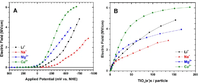
direction of change with increased negative applied potential. ... 49 Figure 2.04. Electric field experienced by Ru(dtb)2(dcb)/TiO2 in acetonitrile
solutions containing 100 mM Li+,Na+,Mg2+,or Ca2+ as a function of (A) the
applied potential and (B) the number of TiO2(e−)s on a per particle basis. ... 51 Figure 2.05. Transient absorption spectra obtained 2.5 μs after pulsed 532 nm
excitation of Ru(dtb)2(dcb)/TiO2 in acetonitrile electrolyte solutions containing 100 mM of the indicated perchlorate salts and 250 mM tetra-n
-butylammonium iodide. ... 52 Figure 2.06. Single-wavelength transient absorption kinetic data of
Ru(dtb)2(dcb)/TiO2 in acetonitrile electrolyte solutions containing 100 mM of the indicated perchlorate salts with 250 mM tetra-n-butylammonium iodide
observed at the maximum of the Stark effect bleach, ∼500−510 nm ... 54 Figure 2.07. Density of states obtained from spectroelectrochemical
measurements of Ru(dtb)2(dcb)/TiO2 sensitized thin films in 100 mM
acetonitrile electrolytes of the indicated perchlorate salts. ... 59 Figure 3.01. Visible absorbance spectra of a Ru(dtb)2(dcb)/TiO2 thin film
immersed in acetonitrile in the absence (gray) or presence of 100 mM LiI
(black), 100 mM NaI (red), 50 mM MgI2 (blue), and 50 mM CaI2 (green). ... 74 Figure 3.02. Absorbance change of Ru(dtb)2(dcb)/TiO2 thin films measured
(A) under conditions of approximately 20 TiO2(e−)s per TiO2 nanoparticle electrochemically generated in 100 mM solutions of NaClO4 (red), LiClO4 (black), Mg(ClO4)2 (blue), and Ca(ClO4)2 (green) and (B) 2.5 μs after pulsed 532 nm light excitation in 100 mM NaI (red, circles) and 50 mM CaI2 (green,
triangles) acetonitrile solutions. ... 75 Figure 3.03. Absorption changes that correspond to TiO2(e−)+ I3−→charge
recombination measured in 100 mM LiClO4 (black), NaClO4 (red),
Mg(ClO4)2 (blue), and mM Ca(ClO4)2 (green) acetonitrile solutions with 250 mM TBAI. Overlaid on the data are fits to the KWW function with β = 0.45. The inset shows a plot of the recombination rate constant versus the electric
field. ... 77 Figure 4.02. Charge extracted from open-circuit over a wide range of voltages,
set by the incident light intensity, for DSSCs containing 100 mM Li+ (Black), Na+ (Red), Mg2+ (Blue), or Ca2+ (Green) perchlorate, 250 mM TBAI, and 50
mM I2. ... 92 Figure 4.03. (A) Transient photovoltage decay measurements for a DSSC
measurements DSSCs containing 100 mM Li+ (Black), Na+ (Red), Mg2+
(Blue), or Ca2+ (Green) perchlorate with 250 mM TBAI, and 50 mM I2. ... 93 Figure 4.04. (A) Transient photocurrent decay measurements for a DSSC
containing 100 mM NaClO4, 250 mM TBAI, 50 mM I2. (B) Diffusion coefficient calculated from the single-exponential decay in transient photocurrent measurements DSSCs containing 100 mM Li+ (Black), Na+ (Red), Mg2+ (Blue), or Ca2+ (Green) perchlorate with 250 mM TBAI, and 50
mM I2 . ... 94 Figure 4.05. Electron lifetimes (A) and diffusion coefficients (B) for DSSCs
containing 100 mM Li+ (Black), Na+ (Red), or Ca2+ (Green) perchlorate with
135 mM CoII(dtb)3(PF6)2, and 15 CoIII(dtb)3(PF6)3 in CH3CN. ... 95 Figure 4.06. Difference between the shift of the TiO2 acceptor state
distribution and the change in Voc relative to Na+ containing DSSCs as a
function of the lifetime relative to Na+. ... 99 Figure 4.07. (A) Electron diffusion coefficient and lifetime as a function of
TiO2(e-)s and (B) diffusion length calculated at matched electron
concentrations for DSSCs containing 100 mM Li+ (Black), Na+ (Red), Mg2+
(Blue), or Ca2+ (Green) perchlorate, 250 mM TBAI, and 50 mM I2. ... 101 Figure 4.08. Dependence of electron lifetime on the relative DoS position for
DSSCs containing 100 mM Li+ (Black), Na+ (Red), Mg2+ (Blue), or Ca2+ (Green) perchlorate, 250 mM TBAI, and 50 mM I2. Circles represent lifetimes measured in I-/I3- containing DSSCs while diamonds represent DSSCs using
CoIII/II redox mediators. ... 104 Figure 5.01. The spectroelectrochemical reduction of the indicated
pyridiniums/TiO2 in 0.1 M TBAClO4 (left hand side) or LiClO4 (right hand
side) CH3CN electrolytes. ... 120 Figure 5.02. The UV/Visible absorption spectra of the indicated pyridiniums
in 0.1 M LiClO4 or TBAClO4 CH3CN electrolyte. ... 122 Figure 5.03. The absorption change for an unfunctionalized TiO2 thin film
measured at 900 nm after a potential step from 0.2 V to the indicated potentials (mV) at time zero in 0.1 M TBAClO4 (left hand side) and LiClO4 (right hand side) CH3CN electrolyte. The potential was stepped back to +0.2
V after 45 s. ... 124 Figure 5.04.The normalized absorption change measured at the reduced
pyridinium maximum wavelength after a step from +0.2 V to the indicated potentials (mV) at time zero in 0.1 M TBAClO4 (left hand side) and LiClO4 (right hand side) CH3CN electrolyte. The potential was stepped back to +0.2
Figure 5.05. UV/Vis absorbance changes for DPEV functionalized TiO2 in 0.1 M TBAClO4/CH3CN during potential steps from +200 mV to -600 mV at time zero and back to +200 mV vs NHE at t = 30 seconds. Single wavelength traces (600 nm) are shown in (A), with close-ups in (C) and (E). Full spectra are shown just before and after each potential step in (D) and (F) to highlight the observation of DPEV+ as an intermediate. Extinction coefficient spectra for DPEV2+, DPEV+, and DPEV0 are shown in (B) for reference. Long wavelength absorption changes in (D) and (F) are caused by the broad
absorption of TiO2 electrons during reduction... 129 Figure 5.06. The chemical capacitance of DPEV2+/+ (blue) and MEV+/0
(purple) and the TiO2 (gray) measured in 0.1 M TBAClO4 (left) and LiClO4
(right) CH3CN electrolyte. ... 130 Figure 6.01. A) Raw and B) normalized absorption difference spectra of
mesoporous, nanocrystalline TiO2 thin film in 100 mM LiClO4 acetonitrile electrolyte at increasingly negative applied potentials ranging from 0 V to -1.5 V vs Fc+/Fc. Overlaid on the normalized spectra in B is the calculated PAS
(black). ... 143 Figure 6.02. A) Raw and B) normalized absorption difference spectra of
mesoporous, nanocrystalline SnO2 thin film in 100 mM Ca(ClO4)2 acetonitrile electrolyte at increasingly negative applied potentials ranging from 0 to -1.5 V vs Fc+/Fc. The inset in A) shows the raw difference spectra from 0 to -700 mV. C) PAS deconvolution of A). D) UV/Vis difference spectra of A) after
returning to the initial potential overlaid with PAS 3. ... 145 Figure 6.03. Absorbance changes monitored at 950 nm for SnO2 (A) and TiO2
(B) thin films in 100 mM Li+ (black), Na+ (red), Mg2+ (blue), Ca2+ (green), and TBA+ (brown) perchlorate acetonitrile electrolyte solutions at the
indicated potentials. ... 147 Figure 6.04. Absorbance change at 900 nm during spectroelectrochemical
charge extraction of TiO2 (A) and SnO2 (B) thin films immersed in 100 mM LiClO4 acetonitrile electrolyte solutions. Charge extracted was normalized by
the geometric area of the thin film. Overlaid in red are linear fits to equation 3. ... 149 Figure 6.05. Cyclic voltammograms of SnO2 (dashed) and TiO2 (solid) thin
films in 100 mM LiClO4 (red) and TBAClO4 (black) acetonitrile electrolyte solutions at a scan rate of 20 mV/s. Currents were normalized by the
geometric area of the thin film. ... 150 Figure 6.06. A) Chemical capacitance for TiO2 (left) and SnO2 (right) thin
films in 100 mM metal perchlorate acetonitrile solutions of Li+ (black), Na+ (red), Mg2+ (blue), Ca2+ (green), and TBA+ (brown). For SnO2 thin films, the smaller distributions represent phantom electrons and the larger
Figure 7.01. STRiVE white and blue LED arrays illuminating a typical DSSC ... 169 Figure 7.02. Relative spectral power distribution of the white LEDs ... 170 Figure 7.03. Relative spectral distribution of colored LEDs. Blue, Green, and
Red are installed on the STRiVE. ... 171 Figure 7.04. (Top) Schematic diagram of the integrated circuit used in the
STRiVE. (Bottom) Picture of the actual board. On the left are MOSFETs used to hold the cell at open/short circuit or allow the potentiostat to be connected
to the circuit. On the right are the amplifiers to accurately measure the current. ... 173 Figure 7.05: Jsc and Voc Set Parameters dialog with typical values shown. ... 178 Figure 7.06: Set iV Curve Parameters dialog showing typical experimental
conditions for a cell with a VOC near 440 mV. ... 180 Figure 7.07. Set Transient Photovoltage Parameters dialog showing typical
values when employed as the first grouped experiment ... 184 Figure 7.08. Set Transient Photocurrent Parameters dialog displaying typical
values when TCD is run as part of a series of grouped experiments (not the
first). ... 188 Figure 7.09. Charge Extraction Experimental Parameters dialog showing
typical values when performed as ‘grouped’ and not the first experiment ... 190 Figure 7.10. Current Interrupt Voltage Parameters dialog with values for
typical operation when performed as a ‘grouped’ (not the first) experiment ... 192 Figure 7.11. Comparison of charge extracted from open-circuit and Voc to the
charge extracted at short-circuit and Vint, the internal voltage calculated from
current interrupt voltage. ... 193 Figure 7.12. Open Circuit Photovoltage Decay Parameters dialog for typical
values when performed in a series of ‘grouped’ experiments (not the first). ... 195 Figure A.01. STRiVE user interface ‘Front Panel’ where the experiments
selected reflect normal operating procedure ... 197 Figure A.02. STRiVE user interface ‘Block Diagram.’ The left and right
rectangles are event structures, which execute only for a user-defined event, such as selecting an experiment or zooming on a graph. In the center is a loop that executes all selected (ungrouped) experiments and then performs grouped
experiments. ... 198 Figure A.03. STRiVE user interface ‘Block Diagram’ selecting the first
Figure A.04. Measure Jsc and Voc ‘Block Diagram’ depicting how VOC is
measured. ... 200 Figure A.05. Measure Jsc and Voc ‘Block Diagram’ depicting how JSC is
measured. ... 200 Figure A.06. STRiVE user interface ‘Block Diagram’ selecting the second
experiment, iV Curve. ... 201 Figure A.07. iV Curve ‘Block Diagram’ Step 1: determine the time to wait
between data points on the curve and connect the potentiostat. ... 202 Figure A.08 iV Curve ‘Block Diagram’ Step 2: run the dark iV curve. This
code is essentially the same as the light-on iV curve. ... 202 Figure A.09 iV Curve ‘Block Diagram’ Step 3: calculate JSc and then VOC and
display the results. ... 203 Figure A.10 iV Curve ‘Block Diagram’ Step 4: plot the dark, light, and power
curves. ... 204 Figure A.11 iV Curve ‘Block Diagram’ Step 5: export the iV data as a .TDMS
file and ensure the potentiostat is set to zero V. ... 205 Figure A.12. STRiVE 5.0 user interface ‘Block Diagram’ selecting the third
experiment, transient photovoltage decay. ... 206 Figure A.13. Transient photovoltage decay ‘Block Diagram’ where multiple
experiments are performed and then the results are collected and plotted. ... 207 Figure A.14. Transient photovoltage decay experimental ‘Block Diagram’
step 1: calculate the sampling parameters. ... 208 Figure A.15. Transient photovoltage decay experimental ‘Block Diagram’
step 2: start with the lights and potentiostat off. ... 209 Figure A.16. Transient photovoltage decay experimental ‘Block Diagram’
step 3: set the light intensity. As shown, a subVI is selected where the
STRiVE finds the light intensity to give a desired VOC. This code is displayed
in Figures A.24-A.27 ... 209 Figure A.17. Transient photovoltage decay experimental ‘Block Diagram’
step 4: set the pulse LED duration. As shown, the STRiVE will find the duration to give a desired ‘Voltage Spike.’ This code is displayed in Figure
Figure A.18. Transient photovoltage decay experimental ‘Block Diagram’ step 5: finalize sampling parameters using the LED pulse time defined in step
4... 211 Figure A.19. Transient photovoltage decay experimental ‘Block Diagram’
step 6: collect the data. This code is found in Figures A.28-29. ... 212 Figure A.20. Transient photovoltage decay experimental ‘Block Diagram’
step 7: turn everything off. ... 212 Figure A.21. Transient photovoltage decay experimental ‘Block Diagram’
step 8: baseline the data and calculate the electron lifetime ... 213 Figure A.22. Transient photovoltage decay experimental ‘Block Diagram’
step 9: display the results and export the data as a .TDMS file. ... 214 Figure A.23. Set light intensity step 0: begin with the user defined current... 215 Figure A.24. Set light intensity step 1: monitor the voltage as the light
intensity is adjusted. The most 3 recent data points are used in a fit to better
approximate the next light intensity output. ... 216 Figure A.25. Set light intensity step 2: set light intensity as the one that was
produced the nearest VOC to the target. ... 217 Figure A.26. Set light intensity step 3: Monitor the voltage for 5 seconds and
check if the equilibrium value is within 5 mV of the target VOC. ... 217 Figure A.27. Set light intensity step 4: Output the light intensity. ... 218 Figure A.28. Transient photovoltage decay Collect Data step 1: equilibrate
with the light on. ... 219 Figure A.29. Transient photovoltage decay Collect Data step 2: use an internal
time ‘counter’ to control the pulse LED and trigger data collection (Reference Digital Edge) that monitors the cell voltage. This process is repeated and
averaged. ... 220 Figure A.30. Transient photovoltage decay ‘Set Voltage Spike’ key code. The
pulse time is adjusted and the transient photovoltage peak is calculated. The
most 3 recent pulses are used to fit and better estimate the required pulse time. ... 221 Figure A.31. STRiVE 5.0 user interface ‘Block Diagram’ selecting the fourth
experiment, transient photocurrent decay. ... 222 Figure A.32. Transient photocurrent decay ‘Block Diagram’ where multiple
Figure A.33. Transient photocurrent decay experimental ‘Block Diagram’ step
1: calculate the sampling parameters. ... 224 Figure A.34. Transient photocurrent decay experimental ‘Block Diagram’ step
2: start at short-circuit but with the light and potentiostat off... 225 Figure A.35. Transient photocurrent decay experimental ‘Block Diagram’ step
3: set the light intensity. As shown the STRiVE will adjust the light intensity to get a defined JSC. This code is very similar to adjusting the light intensity to
set the VOC, Figures A.24-27. ... 226 Figure A.36. Transient photocurrent decay experimental ‘Block Diagram’ step
4: set the pulse LED duration. As shown, the STRiVE will adjust the pulse
time to reach the defined current spike. This code is shown in Figure A.43. ... 227 Figure A.37. Transient photocurrent decay experimental ‘Block Diagram’ step
5: Apply the set parameters... 228 Figure A.38. Transient photocurrent decay experimental ‘Block Diagram’ step
6: collect the data. This code can be found in Figure A.42. ... 229 Figure A.39. Transient photocurrent decay experimental ‘Block Diagram’ step
7: turn everything off and disconnect the potentiostat ... 230 Figure A.40. Transient photocurrent decay experimental ‘Block Diagram’ step
8: baseline the data and calculated the photocurrent lifetime. ... 231 Figure A.41. Transient photocurrent decay experimental ‘Block Diagram’ step
9: plot the data and export the results as a .TDMS file. ... 232 Figure A.42. Transient photocurrent decay Collect Data ‘Block Diagram.’ An
internal time counter is used to define the pulse time and trigger the start of data acquisition. This process is repeated a defined number of times and
averaged. ... 233 Figure A.43. Transient photocurrent decay Set Current Spike ‘Block
Diagram.’ The STRiVE adjusts the pulse time and monitors the current spike. The 3 most recent spikes are fit to more accurately determine the next pulse
time. ... 234 Figure A.44. STRiVE 5.0 user interface ‘Block Diagram’ selecting the fifth
experiment, charge extraction. ... 235 Figure A.45. Charge extraction ‘Block Diagram’ displaying how multiple
experiments are performed and displayed ... 236 Figure A.46. Charge extraction experimental ‘Block Diagram’ step 1: define
Figure A.47. Charge extraction experimental ‘Block Diagram’ step 2: set the light intensity. As shown the STRiVE will find the light intensity for a given
VOC. This code can be found in Figure A24-27. ... 238 Figure A.48. Charge extraction experimental ‘Block Diagram’ step 3: perform
the experiment and average the data. ... 239 Figure A.49. Charge extraction experimental ‘Block Diagram’ step 4:
integrate the current to calculate the charge extracted. This code can be found
in Figure A.52. ... 240 Figure A.50. Charge extraction experimental ‘Block Diagram’ step 5: display
the results and export the data as a .TDMS file. ... 241 Figure A.51. Charge extraction collect data ‘Block Diagram.’ Use the digital
output to switch between open and short-circuit and trigger acquisition. ... 242 Figure A.52. Charge extraction integrate current and calculate charge
extracted ‘Block Diagram.’ ... 243 Figure A.53. STRiVE 5.0 user interface ‘Block Diagram’ selecting the sixth
experiment, current interrupt voltage. ... 244 Figure A.54. Current interrupt voltage ‘Block Diagram’ where multiple
experiments are performed and then the results are collected and displayed. ... 245 Figure A.55. Current interrupt voltage experimental ‘Block Diagram’ step 0:
start at open-circuit with the light only the light on. ... 246 Figure A.56. Current interrupt voltage experimental ‘Block Diagram’ step 1:
set the light intensity. ... 247 Figure A.57. Current interrupt voltage experimental ‘Block Diagram’ step 2:
perform the experiment a defined number of times and average the results.
The code to collect the data can be found in Figure A.61. ... 248 Figure A.58. Current interrupt voltage experimental ‘Block Diagram’ step 3:
display the data. ... 249 Figure A.59. Current interrupt voltage experimental ‘Block Diagram’ step 4:
turn off the potentiostat, lights, and leave cell at open-circuit. ... 250 Figure A.60. Current interrupt voltage experimental ‘Block Diagram’ step 5:
export the data as a .TDMS file. ... 251 Figure A.61. Current interrupt voltage Collect Data ‘Block Diagram.’ An
internal time counter is used to switch between short and open-circuit and
Figure A.62. STRiVE 5.0 user interface ‘Block Diagram’ selecting the
seventh experiment, open-circuit photovoltage decay. ... 253 Figure A.63. Open-circuit photovoltage decay ‘Block Diagram’ where
multiple experiments are performed and then the results are collected and
displayed. ... 254 Figure A.64. Open-circuit photovoltage decay experimental ‘Block Diagram’
step 0: start with everything off. ... 255 Figure A.65. Open-circuit photovoltage decay experimental ‘Block Diagram’
step 1: set the light intensity. As shown the STRiVE adjusts the light intensity
to produce the defined VOC. This code can be found in Figures A.24-27. ... 255 Figure A.66. Open-circuit photovoltage decay experimental ‘Block Diagram’
step 2a: collect data when the spacing between data points is greater than 35 ms. In this case, the end condition can be monitored and the experiment will
stop when met. ... 256 Figure A.67. Open-circuit photovoltage decay experimental ‘Block Diagram’
step 2b: collect data when the spacing between data points is less than 35 ms. In this case, the end condition cannot be monitored and the experiment will
stop when the time is reached. ... 257 Figure A.68. Open-circuit photovoltage decay experimental ‘Block Diagram’
step 3: export the data as a .TDMS file. ... 258 Figure A.69. STRiVE 5.0 user interface ‘Block Diagram’ selecting the
grouped experiment. ... 259 Figure A.70. Grouped experiments ‘Block Diagram’ showing how shared
parameters are set. The rest of the code runs through the experiments similar
LIST OF TABLES Table 2.1. Photophysical and Electrochemical Properties of
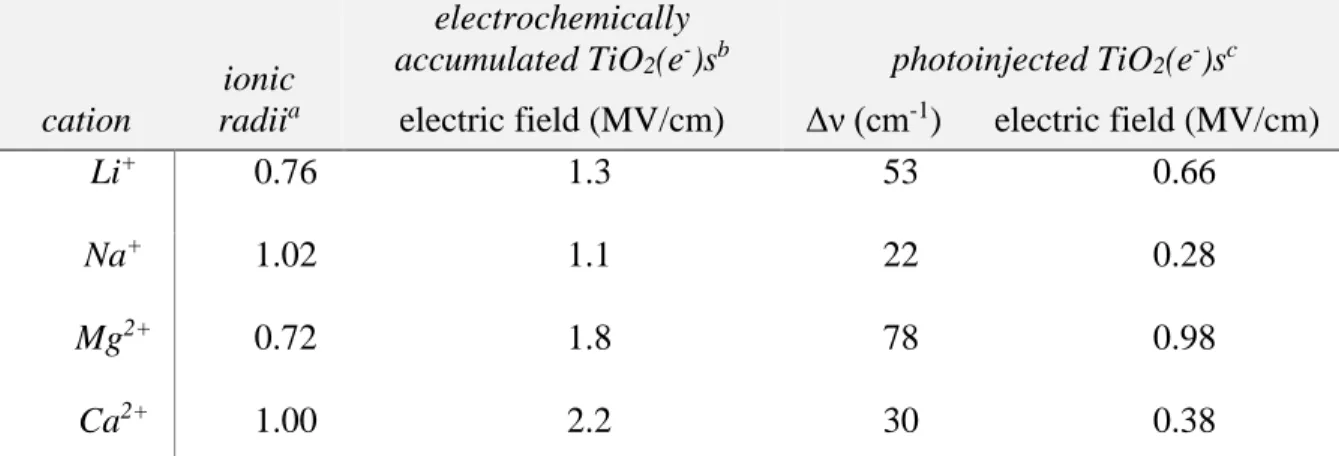
Ru(dtb)2(dcb)/TiO2 in 100 mM Metal Perchlorate Acetonitrile Solutions ... 46 Table 2.2. Ionic Radii, Spectral Shifts, and Electric Field Strength for
Ru(dtb)2(dcb)/TiO2 ... 53 Table 3.1. TiO2(e−)+I3− → Charge Recombination with the Indicated Cations ... 78 Table 4.1. DSSC Figures of Merit from Current-Density Curve in the
Indicated Cations ... 91 Table 4.2. TiO2 DoS, Voc, and electron lifetime values relative to DSSCs in
Na+ electrolyte. ... 98 Table 5.1. Reduction Potentials and Ideality Factors for Pyridiniums in
Solution and Anchored to TiO2 ... 119 Table 5.2. UV/Visible Absorption Properties of the Pyridiniums ... 123 Table 6.1. Absorbance onset potentials for SnO2 and TiO2 thin films in the
indicated 100 mM Mn+(ClO4-)n acetonitrile electrolytes ... 148 Table 6.2. Current onset potentials measured by cyclic voltammetry in the
LIST OF SCHEMES
Scheme 2.1: Structure of Ru(dtb)2(dcb)2+ ... 40 Scheme 2.2. Schematic Depiction of the Light- and Potentiostatically-Induced
Generation of Injected Electrons ... 62 Scheme 4.1. Ru(dcb)(dtb)2(PF6)2 Structure ... 87 Scheme 5.1 Pyridinium structures ... 113 Scheme 5.2. Energetics of the TiO2 Acceptor States Compared to Reductive,
Vred, and Oxidative, Vox, Step Potentials for Interfacial Electron Transfer
LIST OF EQUATIONS
CHAPTER 1: INTRODUCTION
1.1 The case for solar energy
The industrial revolution brought forth unprecedented power through the burning of energy rich fossil fuels that provided ample energy to forever change transportation,
manufacturing, and nearly every aspect of daily life. Such power came with a price: the release of carbon dioxide into the atmosphere at rates never before recorded. Carbon dioxide is a known greenhouse gas, meaning it absorbs infrared light and converts it into thermal energy in the atmosphere. Global temperatures for the past 400,000 years have correlated with CO2 concentration.1 By 1950, CO2 levels had surpassed 300 ppm, a concentration not recorded for the past 400,000 years and in 2016,1,2 the concentration remained above the landmark 400 parts per million (ppm) threshold for the entire year.3 There is ample evidence to show that the Earth is warming: an increase in global temperatures, rise in sea level, shrinking ice sheets, and more frequent extreme weather and all consistent with global warming.4 The financial impact of global warming has already begun, where millions of dollars have been spent relocating people in low-lying regions due to rising sea levels.5,6 Furthermore, CO2 uptake by the ocean acidifies the water that harms marine organisms and corals that are sensitive to small changes in pH.
countries. For example, the United States is expected to consume only ~6.7 % more energy while India is expected to consume ~110 % more energy.7 From an environmental point of view the global increase in energy demand is frightening. The current rate of CO2 release may already lead to irreversible global warming,9–11 making efforts to decrease CO2 production urgently needed.
In order to minimize CO2 release and provide a sustainable future, alternative (non-fossil fuel) sources of power must be developed. Alternative energy sources are unlikely to completely replace fossil fuels as the main source of power in the foreseeable future,
however, they can still have a significant impact by providing the 37 % energy increase that will help keep CO2 production near current levels. One promising source of alternative energy is the sun. Solar illumination provides ~175,000 TW of power constantly to the earth. About 30 % is scattered at 20% absorbed by the surface,12 resulting in ~90,000 TW reaching the surface that has the potential to be harnessed for human use.13 Capturing just 0.015 % of the solar flux could power all current human needs. Using 10 % efficient solar cells, this would require about 0.17% of the earth’s surface. For the United States (~3.3 TW), an area about the size of North Dakota would be required, which is comparable to the land covered by public roads.13
the maximum cell voltage is determined by the bandgap, this single property is critical when designing a solar cell.
Figure 1.01. (A) Solar irradiance measured on the Earth’s surface (terrestrial, black) compared to an ideal blackbody emitter at 5778 K (red). (B) Theoretical power output of a 100 % efficient solar cell absorbing all photons of higher energy than the cutoff value. The maximum power is termed the ‘ideal cutoff.’
Although silicon solar cells are the most common and are decreasing in price rapidly,15 they do not collect diffuse light efficiently, are still relatively expensive, and require high purity materials. An alternative solar cell that excels in all of these areas is the dye-sensitized solar cell. Due to the unique morphology, it collects diffuse light quite well and requires low purity TiO2 as a foundation, which allows for low fabrication costs.
1.2 The dye-sensitized solar cell
The possibility that solar energy could power present and future energy demands and a global awareness of climate change has led to increased public interest in solar power. One device that has received considerable interest over the past 25 years is the dye-sensitized solar cell (DSSC), popularized by Brian O’Regan and Michael Grätzel in 1991.16 The DSSC uses molecular dyes to absorb light and transfer an electron into a wide bandgap
bound dye to absorb (visible) photons and induce a photoelectric effect that was absent without the dye.
Sensitization was first observed over 100 years ago.17,18 Dye-sensitization was studied on TiO2 in the 1970s, but was hindered by the maximum amount of sunlight that could be harvested (< 1%) with a monolayer of dyes on a flat surface.19 Better light absorption was achieved by having thick (~1 µm) dye layers, however this resulted in poor electron collection efficiencies due to the low exciton diffusion length.20 The breakthrough design was to use a mesoporous thin film composed of small (~20 nm diameter) TiO2
nanocrystallites that gave an active surface layer ~1000 times larger than the top down, geometric surface area. This method proved to have both high charge collection efficiencies and high light absorption producing record efficiencies of 7-8 %.16 Two advantages of DSSCs over conventional silicon-based solar cells are the tunability, which is directly controlled by the dye, and the cost of fabrication, which has the potential to be very low due to the low purity requirement and high availability of TiO2.
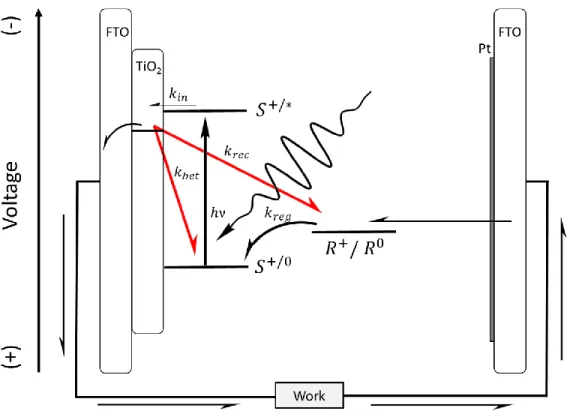
A schematic diagram showing the basic electron transfer processes in a typical DSSC is shown in Figure 1.02. Solar energy is absorbed by the sensitizer to form an excited state on the surface. Excited-state electron injection into the TiO2 acceptor states is often
Figure 1.02. Schematic diagram of the desired (straight/curved black arrows) and unwanted (red arrows) electron transfer processes in a DSSC following light (hν, squiggly arrow) absorption by the sensitizer, S. Also included is a general redox mediator, R+/0, that mediates electron transfer between the oxidized sensitizer and the Pt counter electrode.
Two prominent electron loss pathways exist that prevent all the injected electrons from being collected: back electron transfer to the oxidized sensitizer and charge
known as the electron lifetime, which largely influences the maximum voltage a cell can build under illumination at open circuit.
As with all solar cells, the current is dictated by number of photons absorbed and collected at the back contact. For DSSCs, the number of photons absorbed is determined by the absorptance spectrum of the dye. The open circuit voltage in DSSCs is not dependent on the metal oxide bandgap, but rather the difference between the quasi-Fermi level of the current collectors, often approximated as the TiO2 quasi-Fermi level and the potential of solution the redox mediator. Therefore, what controls current and voltage in a DSSC are decoupled and can be independently optimized. Of note, DSSCs are still a single junction solar cell and have the same thermodynamic limits as silicon single junction solar cells. As such, the ‘ideal cutoff’ of ~1100 nm still holds for DSSCs, where absorbing all light of wavelength shorter than 1100 nm leads to the optimum power. The following sections discuss in more detail some individual components of DSSCs related to this dissertation and how they relate to device performance.
1.3 Description of the electronic states in TiO2
The distribution of electronic states in bulk, single crystal semiconductors is well understood. For metal oxides, the valance band is typically formed by overlap of the oxygen p-orbitals and the conduction band by metal d-orbitals. In an ideal case, the density of states as a function of energy, N(E), shows a parabolic dependence on energy as given by Equation 1.01:23
N(E)= 1 2π2ћ3(2m
*)3/2E1/2
The density of states is position independent within the bulk semiconductor, but is perturbed at the surface when placed in contact with a redox electrolyte. Equilibrium occurs by spontaneous electron transfer across the semiconductor-electrolyte interface until the Fermi levels align. For the case of n-type metal oxides such as TiO2, electrons are usually transferred from the semiconductor to the electrolyte. Excess charge within the
semiconductor is not completely screened due to the low charge carrier density. This results in a space-charge or depletion layer where the majority carrier (electrons) are depleted at the interface relative to the bulk. In the region where the charge is not fully screened, an
‘internal’ electric field within the semiconductor exists such that an electron placed within the semiconductor at the interface would migrate away from the interface towards the bulk.
The electric potential and width of the space-charge layer can be calculated by solving Poisson’s equation with the appropriate boundary conditions. For a flat surface extending infinite distance in the x and y directions, the 1-D Poisson equation has been solved where the voltage and width of the space charge layer as a function of distance from the interface, z, is given in Equations 1.02 and 1.03:
𝑉(𝑧) = −𝑒𝑁𝑑
2𝜀𝜀0(𝑧 − 𝑤)
2 1.02
𝑤 = √2𝜀𝜀0
𝑒𝑁𝑑 1.03
where, e is the (positive) elementary charge, 𝑁𝑑is the number of donors, w is the width of the
space charge layer, ε is the relative permittivity, and ε0 is the permittivity of free space. With typical values for TiO2, 𝑁𝑑 =1017 cm-3 and εTiO2=100, the depletion layer would extend over
The band bending in thin films of ~20 nm diameter TiO2 nanocrystallites used in DSSCs is much different due to the shape and small size of the nanocrystallites. For particles of this size, the width of the depletion layer calculated for a flat interface would be much larger than the particle diameter. Furthermore, the interface of the spherical nanocrystallites are not accurately approximated as an infinitely flat surface. Albery and Bartlett solved Poisson equation for the case for a spherical nanoparticle, which results in the maximum potential difference between the center of the particle of radius r and the surface according to Equation 1.04:24,25
𝑉𝑚𝑎𝑥 =
𝑒 𝑟2 𝑁𝑑 6 𝜀𝜀0
1.04
For typical doping densities of a 1017 cm-3, εTiO2=100, the potential difference between the interface and the center would be less 1 mv, much less than thermal energy, kBT/e≈26 mV. The result is that no conventional, i.e. internal, electric field and no significant band-bending occurs in 20 nm diameter TiO2 nanocrystallites.
The morphological complexity of the nanocrystalline, mesoporous TiO2 thin films with a large number of grain boundaries and surface sites suggests that localized states may be more relevant than carriers in delocalized bonds. Indeed, there appears to be an
Figure 1.03. Theoretical energetic dependence of the density of states, N(E), for a bulk semiconductor (left) and the experimentally observed density of states for mesoporous thin films of ~20 nm diameter TiO2 nanocrystallites (right).
Electrochemical reduction of TiO2 thin films results in population of the acceptor states and charge compensation by the electrolyte cation. However, it is experimentally difficult to ascertain whether the charge compensation mechanism involves cation adsorption to the surface or intercalation into the lattice. The intercalation of Li+ cations is known in occur in bulk26,27 and nanostructured28 TiO2 where the maximum Li/Ti ratio is ½,
present where the TiO2 was able to support the addition of small amount of cations without lattice distortions, however cation adsorption may also have been present.
New insights were gained by carefully monitoring the UV/Vis spectrum of the TiO2 thin film during the application of a negative bias in CH3CN electrolytes.29 When a small amount of charge was transferred to the thin film, broad, superimposable UV/Vis absorption spectra were observed. The spectra bear some similarity to a classical Drude absorption for free electrons in a conduction band, where adjustments due to phonon scattering and ion impurities have been used for TiO2 thin films to account for the discrepancies.30 Furthermore, the spectrum was independent of the identity of the electrolyte cation and was observed with the non-intercalating tetrabutylamminium cation as the charge compensating ion. Therefore, the spectra taken under mildly reducing conditions are attributed to the population of the TiO2 acceptor states without significant cation intercalation. Further reduction of the TiO2 thin films results in a quantitatively different spectrum. The spectrum has a clear peak near 700 nm that is attributed to a more localized transition related to Li+ intercalation into the lattice.29,30
The type of electronic state that is reduced upon application of mild biases is debated in the literature.31,32 The primary differences between the models is the number of electronic states present. One theory is that there are multiple types of states and that the electron is typically localized or trapped, perhaps at a TiIII center, and only transiently occupies a higher lying ‘conduction band’ state. High vacuum (solventless) techniques have provided some evidence for localized TiIII trapped states below a conduction band.33,34 In aqueous electrolytes, a pre-peak is often observed before bulk reduction in cyclic voltammetry
electrolytes, superimposable UV/Vis absorption spectra and a lack of a pre-peak in cyclic voltammograms suggest there is only one type of electron acceptor.
The uncertainty about where the electron resides has become more prevalent when assigning the extinction coefficient of electrons within the thin film. The extinction
coefficient has been measured by comparing the total charge within the film to the optical absorbance and is typically near 1000 M-1cm-1 at 700 nm.30,36,37 However, Hamman and co-workers have recently argued that the absorption feature is due to a small fraction of the total electron concentration that resides in a conduction band, which is distinct from trapped states where the majority of the electrons reside.38,39 Using variable temperature
spectroelectrochemistry, an extinction coefficient of ~10,000 M-1cm-1 for the conduction band electrons was reported. Throughout this dissertation the term ‘acceptor states’ is used to acknowledge the uncertainty in the assignment of the electronic states in nanocrystalline TiO2 thin films.
1.4 Influence of electrolyte cations
Electrolyte pH is known to influence the flatband potential of many bulk metal-oxide semiconductors, including TiO2, SnO2, SrTiO3, ZnO, Zn2TiO4, and KTaO3.40,41 This behavior has been attributed to surface acid/base chemistry related to the protonation state surface oxygen atoms, –O-/-OH. Determining the flatband potential for mesoporous thin films of anatase TiO2 nanocrystallites by the conventional Mott-Schottky approach is precluded by the lack of band bending in the nanocrystallites. Fitzmaurice et. al. applied
electrolyte, indicating the Nernstian behavior of bulk semiconductors extended to nanocrystalline thin films.
When spectroelectrochemical studies were performed in non-aqueous solvents, the identity of the electrolyte cation was found to determine the potential onset where absorption changes were observed.42 Such cations became known as ‘potential determining ions,’ because they determined the energetic position (akin to the flat band potential) of the TiO2 acceptor states. For example, the position of the TiO2 acceptor states was ~1 V more positive in Li+ than TBA+ containing electrolyte, where TBA+ is tetrabutylammonium. The electrolyte cation was thought to be attracted to the negatively charged surface and interact through an adsorption or intercalation mechanism.
Directly related to the energetic position of the TiO2 acceptor states are the electron injection efficiency,43 sensitizer photoluminescence,44 incident-photon-to-current
efficiency,45 and open circuit voltage.45 The rate of electron injection is understood in the framework of Marcus-Gerischer theory according to Equation 1.05:46,47
𝑘𝑒𝑡 =4𝜋 2
ℎ ∫ 𝑔(𝐸)𝑓(𝐸, 𝐸𝐹)|𝐻𝐴𝐵|
2𝑊(𝐸)𝑑𝐸 1.05
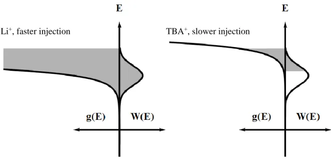
Where g(E) is the distribution of acceptor (TiO2) states, f(E, Ef) is the Fermi-Dirac function that describes the occupancy of the acceptor states, HAB is the electronic coupling element, and W(E) is the distribution of donor states related to solvent fluctuations and the
containing electrolyte, the energetic overlap between the donor states and the TiO2 acceptor states is much greater than in TBA+, as shown in Figure 1.04.
Figure 1.04. Comparison of strong (left, Li+ containing electrolyte) and weak (right, TBA+ containing electrolyte) energetic overlap between the electron donors, W(E), and acceptors, g(E), during charge injection into nanocrystalline TiO2. The area in gray represents regions of favorable energetic overlap.
Marcus-Gerischer theory describes the rate constant for electron transfer, not the overall quantum yield. Once the excited state is formed, a kinetic competition occurs between injection, radiative, and other non-radiative relaxation pathways. A faster charge injection rate constant leads to a greater fraction of excited chromophores relaxing through injection. In the case of ruthenium polypyridyl compounds used in DSSCs, the rate constant is large enough that unit efficiency can often be realized.
An indirect way to monitor electron injection is sensitizer photoluminescence (PL). Electron injection serves as a quenching mechanism for the excited state and decreases the
PL quantum yield. Kelly et. al. monitored sensitizer PL when the cation identity and concentration was systematically varied.43 It was found that the degree of quenching correlated with the charge-to-size ratio of the cation and was consistent with the electrolyte cation tuning the energetic position of the TiO2 acceptor states.
A second indirect measurement of electron injection is the incident-photon-to-current-efficiency (IPCE), sometimes called the external quantum efficiency (EQE). This technique reports the ratio of incident photons illuminating the cell and the number of electrons collected at the back contact. With some assumptions, this serves as a direct
comparison of electron injection efficiency. Comparing IPCE values measured in electrolytes containing Lewis-acidic cations such as Li+ to TBA+ containing electrolytes indicates
significantly less electron injection in TBA+ containing electrolytes as seen by lower IPCE values.45
Figure 1.05. Influence of charge density (left) and energetic position (right) of the TiO2 density of states on open circuit voltage (VOC, double sided arrows). The VOC value can be increased by adding more charge carriers to the film or by increasing the energetic position of the TiO2 acceptor states.
1.5 Interfacial electric fields
In this section the detection and influence of local electric fields at dye-sensitized TiO2 interfaces is discussed. However, it is important to keep in mind that what is typically measured are changes in the electric field following some perturbation. Strong electric fields may exist in the ground state, especially at semiconductor-electrolyte interfaces. These ground-state electric fields are often poorly understood and can cause unavoidably different equilibrium (dark) conditions.
Changes in electric fields, simply referred to hereafter as electric fields, are detected by the UV/Vis absorbance spectra of the dye in what is called an electroabsorption or Stark (sometimes LoSurdo-Stark) effect that was independently discovered by both Johannes Stark and Antonino Lo Surdo in 1913.48–51 Strong electric fields induce shifts in the UV/Vis
absorbance spectrum that reflect the change in transition energy upon stabilization or destabilization of the ground and excited states in the presence of an electric field.52
The extent of (de)stabilization for a single state is usually dominated by the dipole moment, 𝜇⃑, and/or polarizability, 𝛼, of each state according to Equation 1.06.53 The electric field influences both the ground and excited states energies such that the observed change in transition energy corresponds to the difference in dipole moment, ∆𝜇⃑, and polarizability, ∆𝛼, between the two states according to Equation 1.07:53
∆𝐸𝑠𝑖𝑛𝑔𝑙𝑒 𝑠𝑡𝑎𝑡𝑒(𝐸⃑⃑) = −𝜇⃑ ∙ 𝐸⃑⃑ − 1
2𝐸⃑⃑ ∙ 𝛼 ∙ 𝐸⃑⃑
1.06
∆𝐸𝑡𝑟𝑎𝑛𝑠(𝐸⃑⃑) = −∆𝜇⃑ ∙ 𝐸⃑⃑ − 1
2𝐸⃑⃑ ∙ ∆𝛼 ∙ 𝐸⃑⃑
1.07
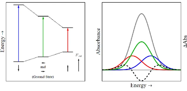
Figure 1.06. (A) Jablonski-type diagram depicting the ground and excited state energies for molecules aligned antiparallel (blue) orthogonal (green) and parallel (red) to the electric field, Fext. Note the transition energy for the orthogonal transition is identical to the ground state transition energy. (B) UV/Vis spectra of an arbitrary transition in the presence of an electric field (gray). Also shown are the individual contributions for molecules oriented parallel (red), orthogonal (green) and antiparallel (blue) to the electric field.
The polarizability represents the ability of a molecule to redistribute its charges in response to an electric field. The polarizability acts as an induced dipole moment or a correction to the constant dipole moment in the presence of an electric field. The redistribution of charge occurs such that the net field across the molecule is minimized, which means that the induced dipole moment is typically aligned with the electric field regardless of the molecular orientation. The result is typically a stabilization of both the ground and excited states, however the magnitude of the stabilization may be different for the two states leading to either a red or blue shift for all molecules, regardless of orientation. Therefore, ‘field-on’ minus ‘field-off’ spectral changes due only to ∆𝛼 can be well-described by the first derivative of the ground state absorption spectrum because the transition energy increases (or decreases) for all molecules.
The electric fields detected in DSSCs represent a unique situation. In these materials, the anchoring of the chromophore to the surface dictates a limited range of binding angles and orientations between the molecule and the surface. Since these electric fields emanate from the surface, the molecules are oriented relative to the field. Every molecules exists in a similar orientation relative to the field which results in similar (de)stabilizations due to ∆𝜇⃑ and ∆𝛼 for all molecules. The resulting spectral shift is unidirectional and well-fit by the first-derivative of the ground state absorption spectrum even for molecules whose change in dipole moment dictate the stark spectrum. To distinguish between shifts caused by ∆𝜇⃑ and ∆𝛼, the field-dependence of the Stark spectrum must be investigated because ∆𝜇⃑ scales with
𝐸⃑⃑ while ∆𝛼 scales with 𝐸⃑⃑2.
metal-to-ligand charge transfer (MLCT) transitions. In the presence of an electric field, changes in the MLCT excitation energy are dominated by ∆µ⃑⃑ associated with transferring an electron from the metal center to a ligand. The peak shift (in wavenumbers, ∆𝜈̃ ) is related to the electric field according to Equation 1.08:
∆𝜈̃ = −|∆µ⃑⃑| ∙ |𝐸⃑⃑|𝑐𝑜𝑠𝜃
100 ℎ𝑐 1.08
Where ℎ is plank’s constant, c is the speed of light, ∆𝜇⃑ is the change in dipole moment between the ground and excited state, 𝐸⃑⃑ is the electric field magnitude, 𝜃 is the angle between ∆𝜇⃑ and 𝐸⃑⃑, and 100 is a conversion factor between m and cm. Due to the broad nature of the MLCT bands, precisely determining the peak maximum (do find ∆𝜈̃) is not always trivial. An alternative means to calculate the electric field is by fitting the difference spectrum to the derivative of the ground state spectrum according to Equation 1.09:
∆𝐴 = −𝑑𝐴 𝑑𝜈
|∆µ⃑⃑| ∙ |𝐸⃑⃑|𝑐𝑜𝑠𝜃 ℎ
1.09
Where ∆A is the difference absorption spectrum and 𝑑𝐴/𝑑𝜈 is the first derivative of the absorption spectrum in wavenumbers. This method generally provides more accurate results as there are more data points in the fit than a single point estimation of spectral shifts. For our calculations, it has been assumed that 𝜃 = 180˚, which corresponds to the electron transfer from the Ru center to the anchoring ligand as normal to the surface.
addition of Li+ to the acetonitrile electrolyte, upon electrochemical reduction of the TiO2 thin film, and following excited-state electron injection into TiO2 nanocrystallites. We will briefly discuss the evidence for electric fields and then several studies reporting the influence
electric fields may have on device performance.
Stark shifts with cation addition: Addition of Lewis-acidic Li+ cations to the electrolyte surrounding a sensitized TiO2 thin film resulted in a large bathochromic (red) shift of both the MLCT absorbance and PL spectrum relative to that in neat CH3CN, consistent with a decrease in the surface electric field.55 The as-synthesized TiO2 nanoparticles are thought to have a negative charge on the surface caused by the deprotonation of surface Ti-OH
groups.56,57 The cationic Li+ ions would be attracted to the negatively charged surface and partially screen the surface electric field.
However, the location of the Li+ cations that screen the field is still unknown. Due to the direction of the shift, it is clear that net electric field reported by the sensitizer is
attenuated indicating the cations reside within the Helmholtz layer, however it is unknown if they interact more directly with the TiO2 surface or the chromophore. It is known that related ruthenium complexes that differ from the compounds discussed here by the protonation state of the carboxylic acid (having deprotonated carboxylates instead of the carboxylic acids here) display similar red shifts upon Li+ addition in fluid solution.58 In fluid solution, the red-shift was attributed to the Lewis-acidic cations interacting with carboxylate groups on the bipyridine ligands, but it was stated that inductive effects could not be
cations reside near the chromophore, but do not outcompete the TiO2 surface for binding to the carboxylate anchoring group.
Stark shift from excited-state electron injection: Nanosecond pulsed laser excitation of sensitized TiO2 thin films immersed in 100 mM LiClO4 and 250 mM tetrabutylammonium iodide (TBAI) results in MLCT excitation and excited-state electron injection into the TiO2 thin film on the fs to ps timescale and then regeneration of the oxidized sensitizer by iodide within 1 µs. The regeneration and recombination reactions were monitored by nanosecond transient absorption spectroscopy. Following sensitizer regeneration, the expected spectral signatures of TiO2(e-)s and triiodide were observed. However, in addition to these expected features, a large first-derivative shape consistent with a Stark shift of the ground-state MLCT transition was observed.55,60,61 This feature was most easily seen when the oxidized
chromophore was regenerated, but has also been identified in previous data from our group and others that did not regenerate the oxidized chromophore.60
Spatial extent of electric field: The discovery of electric fields in dye-sensitized solar cells was surprising to some since macroscopic parameters, i.e. electron diffusion instead of migration within the mesoporous thin films, did not suggest their presence. Perhaps the injected electron resided as a localized electron on a TiIII ion as a ‘trapped electron’ and only effected a single chromophore that did not affect bulk properties. In this light, two studies were conducted to investigate the spatial extent the electric field extended at the interface.
In the first, TiO2 thin films were co-sensitized with two sensitizers whose absorption spectra were distinct enough to permit selective excitation and monitoring of each sensitizer. Selective excitation of one chromophore resulted in excited-state electron injection and sensitizer regeneration. Transient difference spectra recorded at 1 µs after the laser pulse displayed first-derivative features for both sensitizers. This clearly indicated that the electric field extended to laterally across the surface. The magnitude of the spectral shifts indicated that at least two neighboring sensitizers were maximally affected by the electric field, although this result was indistinguishable from a higher number of nearby sensitizers being effected to a lesser extent.
Non-Nernstian redox behavior: The redox behavior of the dyes in dye-sensitized TiO2 thin films has been reported to deviate from the Nernst equation, where a 59 mV change in applied potentials is expected to cause a factor of 10 change in the mole fraction of oxidized and reduced species for a one-electron process.63,64 Instead, it often takes a much larger potential step to achieve a factor of 10 change in the mole fraction. Such data is modelled by the inclusion of an ideality factor, 𝛼, into the Nernst equation, as shown in Equation 1.10. When 𝛼 is unity, Equation 1.10 reduces to the Nernst equation. It has been suggested that a distribution of reduction potentials,65 intermolecular (Frumpkin) interactions,66,67 or electric fields,68 may be responsible for this non-Nernstian behavior.
𝐸 = 𝐸0− 𝛼 59.2 𝑚𝑉 𝑙𝑜𝑔 ([𝑅]
[𝑂]) 1.10
Multiple studies have reported the non-ideal behavior to be surface coverage independent, ruling out Frumpkin-type interactions as the cause for non-ideal behavior. There is no a priori reason to believe there should be a distribution of reduction potentials on the surface, however there is evidence that strong electric fields are present at the surface. If surface electric fields were inducing non-Nernstian redox chemistry, the non-ideality is expected to be sensitive to the magnitude of the electric field. This hypothesis could be tested by studying compounds that underwent multiple one-electron reductions, either at the same or different locations, where the electric field was different for each reduction.
proportional to the number of electrons. In TBA+ containing electrolytes, the TiO2 acceptor states were negative enough that the first and second reduction occurred with minimal change in the TiO2(e-) concentration and the ideality factors were within error the same (although still larger than 1). In Li+ containing electrolytes, the distribution of TiO2 acceptor states were more positive than in TBA+ electrolytes. There were significantly more TiO2(e-)s during the second reduction than the first, corresponding to a larger electric field for the second reduction. A significantly larger ideality factor was observed for the second reduction, consistent with electric-field induced non-Nernstian behavior.
A second study that addressed the electric field influence on non-Nernstian redox behavior utilized a Ru-bridge-TPA, where TPA is triphenylamine, donor-π-acceptor complex where both the Ru center and TPA moiety were redox active. The ruthenium center was bound to the surface and was approximately 15 Å closer than the TPA. Electrochemical oxidation was non-Nernstian at both redox centers, but the Ru center showed on average larger non-ideality than the TPA group. These two examples strongly support that electric fields induce the non-Nernstian redox chemistry on the surface of TiO2.
1.6 Charge transport and recombination in DSSCs:
Charge transport in mesoporous thin films of TiO2 nanoparticles has been measured by a number of techniques, including intensity-modulated photocurrent spectroscopy (IMPS),69 electrochemical impedance spectroscopy (EIS),70–72 pulsed laser transients,73 stepped light-induced transient measurements (SLIM),74,75 and transient photocurrent decay.11,76–79 Likewise, the electron lifetime (inverse of charge recombination rate) has been investigated with intensity-modulated photovoltage spectroscopy (IMVS),80 EIS, 70–72 open-circuity voltage decay,10 and transient photovoltage decay.81 Neither charge transport nor recombination are constant under all operating conditions (incident light intensity). The term ‘effective’ (effective diffusion coefficient or effective electron lifetime) is often used to highlight that the reported values are reported under specific conditions.
Due to the sensitivity of diffusion/recombination on the operating conditions, it has not always been clear how to compare devices, i.e. what independent variable serves as a reference. Early studies found the electron lifetime to exponentially decrease with voltage79 and the diffusion coefficient increase with current.75 Comparisons were therefore made at matched voltage or current values, however this analysis became invalid if the energetic position or density of the TiO2 acceptor states changed between different DSSCs. With the development of several methods to measure the charge within the thin film,82,83 it has become increasingly common to use total charge in the illuminated DSSC as the independent variable when investigating both electron lifetime and diffusion.
DSSCs.11 Dispersive electron transport has been extensively studied for bulk, single crystal semiconductors and is often modelled by a multiple trapping84–87 or continuous-time random walk88–90 mechanism, both of which imply a distribution of bandgap states. More recently, a random flight model has been developed for nanostructured thin films, where a trapped electron can thermally access the conduction band and travel much farther than the nearest neighbor.91 However, most, if not all, recent studies investigating charge transport and recombination in DSSCs are interpreted in the framework of the multiple trapping model as described by Bisquert and Vikhrenko.92 This theory is the basis for comparing kinetic parameters at matched electron concentrations as summarized below.
The foundation of the multiple trapping model is based on multiple types of
electronic states present in the TiO2 thin film. They are often called conduction band states (that contain mobile electrons) and localized states (where the electron are effectively ‘trapped’, 𝑛𝐿). Under steady state conditions, an equilibrium is established between the
conduction band and localized electrons. The number of electrons in the conduction band, 𝑛𝑐,
can be calculated for a given quasi-Fermi level, nEF, using the total number of conduction band states, 𝑁𝑐, and the conduction band energy, Ec, by Boltzmann statistics, Equation 1.11.
The occupancy of trapped states, f, is described by Fermi-Dirac statistics, Equation 1.12:
𝑛𝑐 = 𝑁𝑐𝑒(𝑛𝐸𝐹−𝐸𝑐)/𝑘𝑏𝑇 1.11
𝑓 = 1
1 + 𝑒(𝐸𝐿−𝑛𝐸𝑓)/𝑘𝑏𝑇 1.12
either by a light pulse or a change in the applied bias. This is called the quasi-static approximation and is mathematically represented by Equation 1.13:
𝑑𝑛𝑙 𝑑𝑡 = 𝑑𝑛𝑙 𝑑𝑛𝑐 𝑑𝑛𝑐 𝑑𝑡 1.13
The effective electron lifetime, 𝜏𝑛, of the electron is related to the free electron lifetime, 𝜏0,
according to Equation 1.14, where the final equality holds when 𝑑𝑛𝐿 𝑑𝑛𝑐 ≫ 1:
𝜏𝑛 = (1 +𝑑𝑛𝐿
𝑑𝑛𝑐) 𝜏0 = (1 + 𝑑𝑛𝐿 𝑑𝑛𝐸𝐹
𝑑𝑛𝐸𝐹 𝑑𝑛𝑐 ) 𝜏0
= (𝑘𝐵𝑇 𝑁𝑐 𝑒𝑥𝑝 (
𝐸𝑐−𝑛𝐸𝐹
𝑘𝐵𝑇0 ) 𝑔(𝑛𝐸𝐹)) 𝜏0
1.14
Here, g(nEF) is the distribution of trapped states that is often experimentally observed to increase exponentially with voltage. Equation 1.14 highlights that it is not the absolute voltage (quasi-Fermi level) applied to the cell that determines the electron lifetime, but the difference between the applied voltage and the conduction band energy, (Ec-nEF). The absolute value of the conduction band energy is influenced by the electrolyte and surface bound species. Therefore, comparisons made between different cells are often inaccurate when done at the same voltage because (Ec-nEF) is not the same. Assuming the localized and conduction bands shift together (the relative density and energetic position of the localized and conduction band states is constant), (Ec-nEF) will be matched in different cells when the cells have the same total electron concentration. Since it is difficult to determine the
example), where the concentration of the reacting species must be explicitly taken into account.
As with the electron lifetime, the electron diffusion coefficient, 𝐷𝑛, can be expressed
relative to the free electron diffusion coefficient, 𝐷0, according to Equation 1.15:
𝐷𝑛 = (1 +𝑑𝑛𝐿 𝑑𝑛𝑐)
−1
𝐷0 = (𝑘𝐵𝑇 𝑁𝑐 𝑒𝑥𝑝 (
𝐸𝑐−𝑛𝐸𝐹
𝑘𝐵𝑇0 ) 𝑔(𝑛𝐸𝐹)) −1
𝐷0 1.15
Again it is clear that in this model, comparisons should be performed at matched (Ec-nEF) or total charge. In practice, the same charge often does not coincide with matched operating voltage or incident light intensity. Therefore, measurements are often performed under a wide range of operating conditions and compared over similar values in electron
concentration.
Knowing the diffusion coefficient and electron lifetime, the diffusion length, 𝐿𝑛, defined to be the average distance an electron travels in the thin film before recombination, can be calculated. This model predicts a constant diffusion length according to Equation 1.16.
𝐿𝑛 = √𝜏𝑛𝐷𝑛 = √𝜏0𝐷0 1.16
Reports of the diffusion length as a function of voltage are often observed to generally follow this model, i.e. are constant, however slight differences are often observed that have been attributed to nonlinear recombination or recombination from trapped states.93–95
been several reports of how to relate 𝐿𝑛 to collection efficiency, 𝜂, shown in Equations 1.17-1.19:96
𝜂 = 𝐿
𝑑𝑡𝑎𝑛ℎ ( 𝑑
𝐿) 1.17
𝜂 = 1 −𝜏𝑐,𝑛
𝜏𝑣,𝑛 1.18
𝜂 = 1 −𝜑𝑜𝑐(𝑉)
𝜑𝑠𝑐(𝑉) 1.19
where 𝜏𝑐,𝑛 and 𝜏𝑣,𝑛 and the transient photocurrent and photovoltage lifetimes at electron concentration n, respectively, and 𝜑𝑜𝑐(𝑛) and 𝜑𝑜𝑐(𝑛) are the incident light intensities to generate a given electron concentration within the TiO2 thin film at open circuit and short circuit, respectively. These methods generally agree for 𝐿𝑛/d > 2, which corresponds to ~90 % charge collection efficiency, but differ when significant losses occur. It is unclear how a constant diffusion length calculated this way is reconciled with several reports that the collection efficiency decreases at the power point or under open circuit conditions of DSSC.21,22 It is possible that these authors observed a relatively small fraction of injected electron recombine prior to their impact on transient electronic techniques that measure the response at the collecting substrate.
Investigating the electron lifetime and diffusion coefficient as a function of total charge within the thin films provides a ‘snapshot’ of the fundamental processes governing cell efficiency. During the course of my Ph.D. studies I built an instrument, termed STRiVE for “Sequential Time-Resolved current (i) Voltage Experiments,” that is capable of