SHAPE
DEFORMATION
STATISTICS AND
REGIONAL
TEXTURE
-BASED
A
PPEARANCEM
ODELS FORS
EGMENTATIONJared Vicory
A dissertation submitted to the faculty of the University of North Carolina at Chapel Hill in partial fulfillment of the requirements for the degree of Doctor of Philosophy in the Department
of Computer Science.
Chapel Hill 2016
c 2016 Jared Vicory
ABSTRACT
JARED VICORY: Shape Deformation Statistics and Regional Texture-Based Appearance Models for Segmentation.
(Under the direction of Stephen M. Pizer)
Transferring identified regions of interest (ROIs) from planning-time MRI images to the trans-rectal ultrasound (TRUS) images used to guide prostate biopsy is difficult because of the large difference in appearance between the two modalities as well as the deformation of the prostate’s shape caused by the TRUS transducer. This dissertation describes methods for addressing these difficulties by both estimating a patient’s prostate shape after the transducer is applied and then locating it in the TRUS image using skeletal models (s-reps) of prostate shapes.
First, I introduce a geometrically-based method for interpolating discretely sampled s-reps into continuous objects. This interpolation is important for many tasks involving s-reps, including fitting them to new objects as well as the later applications described in this dissertation. This method is shown to be accurate for ellipsoids where an analytical solution is known.
Next, I create a method for estimating a probability distribution on the difference between two shapes. Because s-reps live in a high-dimensional curved space, I use Principal Nested Spheres (PNS) to transform these representations to instead live in a flat space where standard techniques can be applied. This method is shown effective both on synthetic data as well as for modeling the deformation caused by the TRUS transducer to the prostate.
method is shown to be able to accurately discern inside appearances from outside appearances over a large majority of the prostate boundary.
ACKNOWLEDGMENTS
TABLE OF CONTENTS
LIST OF FIGURES . . . x
LIST OF ABBREVIATIONS . . . xi
1 INTRODUCTION . . . 1
1.1 Image-guided Prostate Biopsy . . . 2
1.2 Segmentation of the Prostate from TRUS . . . 3
1.3 Skeletal Representations . . . 3
1.4 Statistics on Shape Differences . . . 4
1.5 Appearance via Regional Texture Classifiers . . . 5
1.6 Interpolation of Discrete S-reps . . . 6
1.7 Thesis & Contributions . . . 6
2 BACKGROUND. . . 9
2.1 Object Representations . . . 9
2.1.1 Point Distribution Models . . . 9
2.1.2 Skeletal Representations . . . 9
2.2 Statistical Methods . . . 10
2.2.1 Principal Component Analysis. . . 10
2.2.2 Non-linear Statistical Methods. . . 11
2.2.3 Principal Nested Spheres . . . 13
2.2.4 Composite Principal Nested Spheres . . . 13
2.2.5 Appearance Models and Segmentation . . . 14
2.2.6 Appearance-based Segmentation . . . 14
3 CONTINUOUS INTERPOLATION OF SKELETAL REPRESENTATIONS . . . 19
3.1 Introduction . . . 19
3.2 Mathematics of Skeletal Representations . . . 21
3.3 Skeleton Interpolation . . . 23
3.4 Spoke Interpolation . . . 24
3.5 Estimation of Spoke Direction Derivatives via Quaternion Splines . . . 26
3.6 Interpolation of the Crest . . . 28
3.7 Spoke Computation via Integration of Derivatives. . . 29
3.8 Discussion . . . 30
4 PROBABILITY DISTRIBUTION ESTIMATION OF SHAPE DIFFERENCES. . . 31
4.1 Introduction . . . 31
4.2 Related Work . . . 32
4.3 Methodology . . . 33
4.3.1 Euclideanization . . . 33
4.3.2 Probability Distribution Estimation. . . 34
4.4 Evaluation . . . 34
4.4.1 Single Mode of Change . . . 35
4.4.2 Composed Bending and Twisting . . . 36
4.4.3 Application to S-reps . . . 37
4.5 Discussion . . . 37
5 MODELING TRUS APPEARANCE VIA REGIONAL TEXTURE CLASSIFIERS . . . 40
5.1 Introduction . . . 40
5.2 Materials . . . 41
5.3 Methodology . . . 42
5.4 Application. . . 43
5.5 Evaluation . . . 44
5.6 Discussion . . . 45
6 SEGMENTATION OF THE PROSTATE FROM TRUS . . . 47
6.1 Introduction . . . 47
6.2 Materials . . . 47
6.3 Segmentation Methodology . . . 47
6.3.1 Model Deformation and Probability . . . 48
6.3.2 Probability Images and Image Match. . . 49
6.3.3 Optimization . . . 50
6.4 Results . . . 50
6.4.1 Estimation of Prostate Deformation Distribution . . . 50
6.4.2 Segmentation . . . 50
6.4.3 Refinement . . . 51
6.5 Discussion . . . 52
7 CONCLUSIONS & DISCUSSION . . . 54
7.1 Discussion and Future Work . . . 55
7.1.1 S-reps and Fitting . . . 55
7.1.2 Interpolation . . . 56
7.1.3 Statistics on Shape Differences . . . 57
7.1.4 Appearance Model . . . 58
7.1.5 Segmentation . . . 58
7.1.6 Conclusions . . . 60
LIST OF FIGURES
2.1 Euclidean vs non-Euclidean mean . . . 12
2.2 PNS projection example . . . 13
3.1 Usefulness of s-rep interpolation for fitting . . . 19
3.2 S-rep spoke-relative dilation . . . 23
3.3 Interpolated s-rep skeletal sheet. . . 24
3.4 S-rep interpolation quad . . . 25
3.5 De Casteljau’s algorithm . . . 27
3.6 Crest curve dilation for interpolation . . . 29
3.7 An interpolated s-rep . . . 30
4.1 Estimated bending and twisting angles . . . 35
4.2 Difference between PCA- and CPNS-estimated deformations . . . 37
4.3 Mean deformations applied to s-reps . . . 38
4.4 S-rep deformation eigenmodes. . . 39
5.1 Fanned and unfanned ultrasound images . . . 44
5.2 Ultrasound intensity and texture images. . . 44
5.3 DiProPerm z-scores . . . 45
5.4 Path misclassification rates . . . 45
6.1 Prostate probability image . . . 49
6.2 Prostate pre- and post-deformation . . . 51
LIST OF ABBREVIATIONS
CPNS Composite Principal Nested Spheres DSC Dice Similarity Coefficient
DWD Distance-weighted Discrimination GPCA Geodesic Principal Component Analysis
LDDMM Large Deformation Diffeomorphic Metric Mapping MAD Mean Absolute Distance
MRI Magnetic Resonance Imaging MSE Mean Squared Error
PCA Principal Component Analysis PDM Point Distribution Model PGA Principal Geodesic Analysis PNS Principal Nested Spheres ROI Region of Interest
1 INTRODUCTION
The driving problem for the work in this dissertation is segmentation of the prostate in 3D trans-rectal ultrasound (TRUS) during an image-guided biopsy procedure. The main task is to identify the prostate and certain regions of interest (ROIs) identified during pre-biopsy planning. This problem presents several challenges, including
1. Low contrast between the prostate and surrounding tissue
2. High noise and noise-like (speckle) artifacts present in ultrasound 3. Highly varying appearance around the prostate boundary
4. Deformation of the prostate caused by the TRUS transducer
The first three items combine to make segmentation of the prostate challenging using standard tech-niques which may work well in other imaging modalities. The fourth makes using prior knowledge of the shape of a particular patient’s prostate gained during planning difficult as well as locating corresponding regions of the prostate post-deformation.
I argue that a method designed to solve this driving problem needs
1. A model of shape that supports
• identification of corresponding local regions across multiple cases
• continuous representation of both the boundary and interior of the prostate
2. An appearance model that
• uses features suitable for analysis of ultrasound appearance, especially texture
3. Statistical analysis of the differences between pairs of shapes
This dissertation describes novel methodological contributions in each of these areas. The following sections further develop the driving problem and the intuition behind each of the items listed above.
1.1 Image-guided Prostate Biopsy
Prostate cancer is the most commonly diagnosed cancer among adult men (excluding basal cell carcinoma) and is the second leading cause of cancer death among men in the United States [1]. Early diagnosis is important for improving survivability of prostate cancer. The standard method for obtaining this diagnosis is through a TRUS-guided biopsy of the suspected cancer.
Often, the ROIs for the biopsy procedure are identified on an MRI of the pelvis. On MRI there is typically good contrast in the soft tissue and relatively easy detection of ROIs. During the biopsy procedure the available TRUS images are of very different appearance and quality than the planning MRIs, making accurate identification of the ROIs difficult. Compounding this problem is the fact that the TRUS transducer puts pressure on and deforms the prostate, causing it to have a different shape compared to planning-time. These factors make TRUS-guided biopsy error-prone and can lead to missing a significant fraction of cancers. In order to improve the accuracy of the biopsy procedure, it is important to be able to accurately identify not only the prostate boundary in TRUS but also regions of the prostate which correspond with MRI-identified ROIs.
1.2 Segmentation of the Prostate from TRUS
Segmentation of the prostate in TRUS is most effectively done by analyzing the texture of the image, whether on a global or local scale. Many of these methods also include some type of shape prior in order to keep the segmented shape regular. Point distribution models (PDMs) [3] are commonly used in shape-informed segmentation methods for the prostate as well as many other organs throughout the body. These methods will often learn statistics on a population of PDMs using principal component analysis (PCA) and restrict the set of candidate shapes to the space of shapes spanned by some number of eigenmodes of this learned distribution.
PDMs have several useful properties, including ease of model creation, simplicity of represen-tation, and straightforwardness of various computations involving their representation. The geom-etry captured by PDMs, however, is somewhat limited, particularly when restricted to boundary points only (as is often the case). Boundary PDMs capture only 0th-order information about the object’s surface explicitly and thus lack higher-order information such as boundary normal direc-tions or surface curvatures. These can be estimated if the surface has connectivity information, but the accuracy will be limited by the sample density. Boundary PDMs also do not explicitly model the object interior, which is important for applications needing corresponding locations in the object’s interior.
1.3 Skeletal Representations
position information about the object’s surface. This representation has been shown to be superior to boundary PDMs for uses such as classification [5] and estimating object correspondences. [6].
Due to the non-Euclidean nature of most of an s-rep’s features, standard Euclidean statistical methods such as PCA are not directly applicable to s-reps. Instead, an alternative approach called
Euclideanizationis used to turn these non-Euclidean features into Euclidean ones to which stan-dard methods can then be applied. This Euclideanization of the sphere-resident features is done via principal nested spheres (PNS), which analyzes the s-rep features on the abstract spheres they naturally live on. Performing PCA on these Euclideanized features yields an s-rep shape space which can be used for segmentation as described previously.
1.4 Statistics on Shape Differences
As mentioned previously, the TRUS transducer causes the shape of the prostate to deform from what is observed on the planning MRI. In segmenting the prostate from TRUS, I wish to leverage information learned from a patient’s MRI. For this, it is not enough to simply learn a distribution of shapes of the prostate post deformation; we must also learn how the transducer causes the prostate to deform.
Given an MRI/TRUS image pair for a specific patient and manual segmentations of the prostate, I can learn the transducer-induced deformation by fitting consistent s-reps to both segmentations and computing a deformation from the MRI to the TRUS models. Given a population of such pairs, a probability distribution of these shape changes can be learned. To do this in a meaningful way, both the deformations and the probability distribution must be computed while keeping the non-Euclidean nature of s-reps in mind.
difficult and expensive to compute. Moreover, given a population of geodesics on the manifold, they must first be transported to a common starting point before they can be compared, a far from trivial task except in spaces where a closed-form solution is known.
Instead, because the exact structure of the manifold s-reps live on is known and there are statisti-cal methods capable of analyzing them directly on this manifold, I again apply the Euclideanization idea to computing the difference between two s-reps. Taking the pooled group of MRI and TRUS prostate models, I compute PNS and thus a common polar system for Euclideanization. Then, the Euclideanized s-reps can be directly analyzed in Euclidean space as described previously, yielding a mean deformation and modes of deformation variation.
Given a new patient’s manually segmented MRI, I can apply this mean deformation to yield a patient-specific intialization for the prostate’s shape in the TRUS image and deform it over these modes of deformation variation to better match the image using some model of the prostate’s appearance in TRUS.
1.5 Appearance via Regional Texture Classifiers
Analyzing the appearance of an organ in ultrasound imaging is a difficult task. Relying on intensity information alone is unsatisfying because of issues of low contrast between neighboring organs as well as the noise-like speckle artifacts found in ultrasound images. Instead, texture fea-tures are often used to model the appearance of the prostate in TRUS images. Gabor filters, either 2D or 3D, are a common choice for this task. I compute texture using 48 oriented Gabor features which, together with the smoothed image intensity, yields a 49-tuple of appearance information at each image voxel.
robust to the changes in TRUS appearance around the prostate than methods which model texture globally or using large regions of the image.
I learn these local texture profiles by, about each spoke, pooling texture features from just inside and just outside the prostate boundary into two classes and training a classifier to distinguish between them. For a new case to be segmented, we apply these classifiers to the voxels near the boundary of a candidate object and optimize the model so that more likely inside voxels are inside the boundary and vice versa.
1.6 Interpolation of Discrete S-reps
For many applications, including the segmentation problem here, it is desirable to have a more finely sampled s-rep than the base model. This is desirable for fitting an s-rep to an object. It is also used for representing an object in terms of object-relative coordinates, which is an important component for producing regional appearance models for segmentation. These objectives require the development of a method for continuously interpolating a discrete s-rep. Building on the calculus of skeletal models, I develop a geometry-based method for interpolating an s-rep into a continuous object while maintaining its useful geometric properties.
1.7 Thesis & Contributions
Thesis:Segmentation of an object deformed from a base state in a systematic way with appear-ance that varies around its boundary benefits from combining the following two approaches:
1. Statistical analysis of the object deformation by a method suited for analysis in curved spaces
2. Regionally trained appearance models to distinguish voxels inside and outside of the object’s
boundary.
Instead of the more typical boundary-based approach, continuously interpolated skeletal models
form a strong basis for the training of statistics of object deformation as well as the creation of
object-relative regions on which to train appearance models.
1. A geometric interpolation method for computing continuous skeletal models from discrete s-rep models.
2. A method for computing a probability distribution of differences between pairs of shapes which leverages the non-Euclidean nature of shape and shape representations.
3. A novel appearance model which leverages the ability of the s-rep to produce corresponding local regions around an object to define local classifiers of image texture.
4. The application of the aforementioned techniques in a deformable model-based segmenta-tion method for segmenting the prostate from TRUS.
In addition to these, I have also accomplished the following engineering contributions:
1. Implementation in Pablo, the main piece of software used to fit and visualize s-reps, of code allowing optimization over a shape space defined by CPNS
2. Implementation in Pablo of spoke interpolation in both the display and fitting of s-reps
3. Implementation of code to compute and optimize over spaces of shape differences
4. Implementation to compute regional classifiers of inside/outside boundary appearance fea-tures and computation of images of probability of being inside and object
5. Implementation in Pablo of code allowing optimization of a model to best fit a probability image, including both optimization over a global shape space and local refinements
6. Numerous bug fixes and improvements to Pablo
2 BACKGROUND
This section covers information which is common background information for each of the following chapters. Background information specific to only one chapter can be found there. 2.1 Object Representations
2.1.1 Point Distribution Models
Point distribution models (PDMs) are shape models which are a collection of points which are in corresponding locations on each object of a population. Though they are often formed using only boundary points, they are not restricted to be so. There are several methods for producing PDMs from a set of objects, including manual placement of landmarks, automatic generation of corresponding points such as SPHARM-PDM [7], and methods for optimizing the correspondence of existing models such as the entropy-based method of Cates [8].
2.1.2 Skeletal Representations
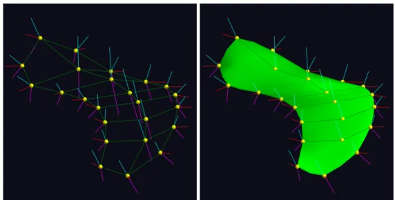
The s-rep is a quasi-medial skeletal model that models not only an objects boundary but its interior as well. The s-rep is a collection of points sampled from a skeleton of an object which have associated non-crossing vectors called spokes pointing from the skeleton to the objects boundary. S-reps attempt to be as close to medial as possible while remaining non-branching and require the spokes to touch the object boundary and be nearly orthogonal to it. These samples can then be interpolated via the method described in chapter 3 to produce a continuous representation of an objects boundary and interior. This provides an object-relative coordinate system(u, v, τ)for the objects volume, where(u, v)parameterizes the skeleton andτ moves from the skeleton (τ = 0) to the boundary (τ = 1).
a template model into an invidual case via a thin plate spine (TPS) interpolation of the boundary correspondences of the template object and the target object followed by an optimization which more closely matches the spokes to the object’s boundary. For producing these correspondences, I use the thin shell demons [9] method to register a reference PDM to a target PDM and use the implied correspondences to fuel the TPS warping.
In the past several years, s-reps have been shown to be powerful and in most cases superior to PDMs for a variety of statistical tasks, including hypothesis testing [10], classification [5], and producing corresponding objects [6].
2.2 Statistical Methods
2.2.1 Principal Component Analysis
Principal component analysis (PCA) is an important statistical procedure designed to be used for probability distribution estimation and dimensionality reduction of Euclidean data. The result of PCA on data of dimension d can be understood as the fitting of a d-dimensional Gaussian distribution to the data.
PCA can operate in either a forward or backward manner, the results of which are equivalent for Euclidean data. In the typical forward approach, the first step is to compute the mean of the data, which is the best fitting linear subspace of dimension 0. The line through the mean which minimizes the sum of the squared projections of each data point to the line, the best-fitting subspace of dimension1, is called the first principal component. Next, the plane containing the first principal component which minimizes the projection error is computed. The vector contained by this plane which is orthogonal to the first principal component is the second principal component. This procedure of fiting the best-fitting linear subspace of successively increasing dimension is repeateddtimes.
untild−1 = 0, yielding a mean. In this approach, PCA can be thought of as a successive addition of constraints to the original data rather than a construction of best-fitting lines as in the forward approach. In a Euclidean space both approaches yield the same result, but this property does not hold in general.
PCA can be computed by an eigendecomposition of the data covariance matrix. When sorted from largest to smallest eigenvalue, the corresponding eigenvectors represent the principal com-ponents in decreasing order, while the eigenvalues represent the variances of the 1-dimensional Gaussians in orthogonal spaces which compose the overall distribution.
One of the most important characteristics of a PCA-generated probability distribution is having as few large eigenvalues as possible given the data being analyzed. This typically indicates that the data are well represented by a small number of linear subspaces, yielding strong dimensionality reduction with low loss of information.
2.2.2 Non-linear Statistical Methods
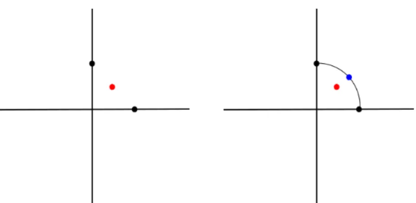
PCA is a powerful analysis technique, but it assumes that the underlying data are samples from some distribution on a flat space. However, if the data are instead samples from some curved man-ifold, this assumption often causes PCA to produce distributions with many significant eigenval-ues, meaning that many dimensions are needed to keep information loss adequately low. Modeling manifold data using linear subspaces also yields data points outside of the original manifold. Fig-ure 2.1 shows a simple example of computing the mean of two data points sampled from an arc of a circle. In this case, the mean computed via a metric which knows about the manifold’s structure is more appropriate than the traditional Euclidean mean.
Figure 2.1: On the left, without knowledge of the data’s original manifold, the Euclidean mean (red point) is a good approximation. On the right, knowing the data are samples from an arc, the mean using the manifold’s metric (blue point) is more reasonable.
Because of this, methods which can analyze data directly on their manifold are desired.
A popular method for analyzing data on a curved manifold is principal geodesic analysis (PGA) [12]. In its most common form, PGA computes a mean of the data on the manifold. Then, all of the data is mapped onto the tangent plane at the mean and PCA is computed on this projected data.
Geodesic PCA (GPCA) [13] is a method which works similarly to PGA, but instead of using PCA in the tangent space it instead minimizes projection error to geodesics on the manifold itself. This method has the drawback that it needs explicit formulas for manifold geodesics, which are often not available.
PGA and related methods work on data which live on some manifold which may not be easy to work with directly. In cases where the underlying manifold is known, however, approaches which can use this knowledge directly can produce more accurate and efficient results. Many shape representations either are or are composed of data which live on abstract spheres, such as PDMs [14] and s-reps [4].
Because so many of these features are spherical, a method tailored to analyzing spherical data is desirable.
2.2.3 Principal Nested Spheres
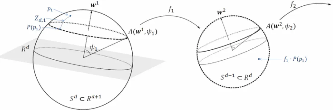
Principal nested spheres (PNS) [15] is a method that operates in a PCA-like backwards fashion on spherical data. Starting fromSd, the best-fitting subsphereSd−1is computed and represented as a polewand angleψ. Each pointpiis projected onto the subsphere, and the process is repeated on each subsphere until a single point, the backwards mean, is reached. At each projection step, the signed geodesic distanceZd,1 from each point to the fit subspace is recorded, yieldingdresiduals
for each data point. These residuals are called the Euclideanized form of the data, while the collection of poles and angles defining the subspheres form a polar systemwhich can be used to Euclideanize a new shape via this repeated projection. A Euclideanized shape can be returned to its original ambient space by undoing these projections to recover the original representation. Figure 2.2 shows an example PNS step.
Figure 2.2: An example projection step from a PNS analysis. The point p1 is projected onto the
subsphere defined by the polar systemA(w1, ψ
1). The projection distanceZd,1is a Euclideanized
feature.
2.2.4 Composite Principal Nested Spheres
the hub PDM and one for each s-rep spoke direction. For each s-rep, the resulting Euclideanized values are combined with the log-transformed spoke lengths into a single vectorZ in a step called compositing. The collection of Z vectors for a population of s-reps can then be analyzed using PCA. This technique is known as composite principal nested spheres (CPNS).
Experimentally, it has been shown that s-rep features, particularly spoke directions, tend to lie on or near subspheres and are thus well modeled via PNS. CPNS has been shown to produce more efficient representations and statistics for both PDMs and s-reps than either PCA or PGA, leading to improved performance in tasks such as hypothesis testing [10] and classification [5]. These results indicate that CPNS-based Euclideanization is a powerful technique for the analysis of s-reps.
2.2.5 Appearance Models and Segmentation
In this section, I discuss previous work on how to model image appearance for segmentation, focusing on methods used for ultrasound prostate segmentation. I divide the methods into two broad categories: those that attempt to segment an object via appearance directly, and those that combine image information with some type of deformable model to perform segmentations. Full surveys of prostate segmentation methods can be found in [16] and [17].
2.2.6 Appearance-based Segmentation
in the ultrasound image by using the fact that speckle is correlated over large distances. Mahdavi et al. [20] use measures of edge strength in vibro-elastography (VE) ultrasound images rather than typical B-mode images to perform segmentation. A common approach in all imaging modalities to smooth image intensity while preserving edges is to use an anisotropic diffusion filter. In my work on modeling ultrasound appearance in chapter 5, I use the speckle-reducing anisotropic diffusion method of Yu et al.[21] to get smoothed ultrasound images.
Graph-based segmentation algorithms model image voxels or groups of voxels as nodes in a graph. The edges linking a voxel to its neighbors have an associated cost, typically related to the gradient of the image. The image is segmented by trying to cut the graph into different pieces while minimizing the cost of these cuts. Zouqi et al. [22] used graph partitioning to segment the prostate with the user defining seed points which act as the sink and source nodes for a max flow optimziation. Qiu et al. [23] segment the prostate using a coherent continuous max-flow model which enforces geometric consistency across multiple 2D slices to segment the prostate in 3D.
determining the mean and covariance for each of a set of clusters and assigning a probability to each voxel for each cluster. The object boundary was then refined using spatial information, with spatially close voxels being more likely to have come from the same cluster.
2.2.7 Model-based Segmentation
The class of methods described in section 2.2.6 attempt to capture the boundary of an object purely by considering its appearance and attempting to separate it from surrounding tissue. While they have been successful in many applications, methods of this class can result in segmentations which are non-smooth or possibly not even continuous, especially if they are working on a voxel-by-voxel basis rather than considering spatial locality. To combat this problem, these methods can be supplemented by models which can deform to match a boundary located by analyzing an image’s appearance. Regularity constraints can be used in order to ensure that the resulting boundaries are smooth and continuous while still closely matching the object of interest.
Surface Detection [34] segmentation. Ladak et al. [35] and Ding et al. [36] improve on the initial ACM by using more sophisticated spline-based techniques for connecting the control points and thus improving the smoothness of the boundary.
Active shape models (ASM) [3] were proposed to counter the weakness of other model-based methods that the resulting boundaries can often be atypical of the shape of the object being seg-mented. ASMs work by performing statistical analysis (most commonly PCA) of PDMs of cor-responding landmarks across a population of shapes. The modes of variation resulting from PCA form a shape space over which the mean PDM can be deformed to better match image data while still remaining consistent with the shape of the object in question. This prior shape informa-tion makes the resulting segmentainforma-tions more robust to noise and artifacts. Shen et al. [37] used rotation-invariant Gabor features to both smooth and detect prostate edges. They then segmented the prostate using an ASM by refining it at multiple scales. Betrouni et al. [38] enhanced the prostate edge using prior knowledge of the noise distribution of TRUS images. Zhan et al.[39] use classifiers trained on Gabor filter-derived features to divide texture space into prostate and non-prostate regions to drive a deformable segmentation of the non-prostate. In later work, Zhan et al.[40] use locally-trained classifiers learned on Gabor texture features to classify regions of the image as prostate or not to guide an ASM. Cosio et al. [41] used a Gaussian mixture model to cluster prostate and non-prostate tissues and used a Bayesian classifier to identify prostate voxels followed by an ASM-based segmentation.
Active appearance models (AAM) [42] are models which statistically model not only an ob-ject’s shape but its appearance as well in a joint fashion. Medina et al. [43] used AAM segment the prostate. Ghose et al. [44] used approximations via Haar wavelets to reduce speckle and contrast-invariant texture features to improve AAM segmentation accuracy.
Tutar et al. [45] use statistics computed on spherical harmonic coefficients together with derived edge maps to segment the prostate.
These methods work by constructing an atlas from a set of manual segmentations. Segmentation is performed by deforming the atlas image to better match a target image. In this way, atlas-based segmentation can be treated as a registration problem. Yang et al.[46] computed Gabor filters in three orthogonal planes and classifiers were trained on six image subvolumes. Segmentations were then performed by warping atlas images to the target image and applying subvolume classifiers to enhance the segmentation. Atlas-based segmentation of the prostate must often be refined via a separate deformable model to improve accuracy, such as in the method of Martin et al.[47].
3 CONTINUOUS INTERPOLATION OF SKELETAL REPRESENTATIONS
3.1 Introduction
Discrete s-reps have been shown to be powerful shape representations for a variety of tasks. Tasks involving statistical analysis often analyze the s-rep’s sampled representation directly. How-ever, other applications such as s-rep fitting and s-rep-based segmentation benefit from having a continuous model rather than operating from these samples alone.
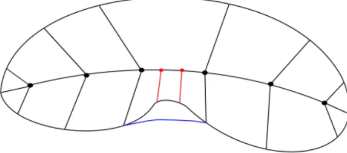
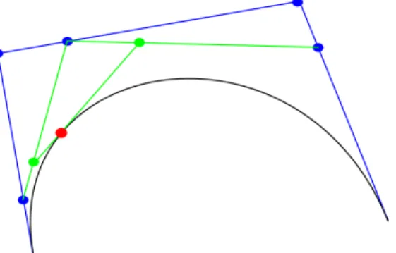
Consider the fitting case in figure 3.1, where an s-rep is being fit to an object boundary (black). If fitting is done considering only how well the s-rep matches the object at the base s-rep spokes, the resulting s-rep implied boundary (blue) will miss the bump in the object surface. If, however, the fit is done using interpolated spokes (red), the optimization will have to shift the base spokes to better model this bump, thus increasing accuracy of the fit. Similarly, segmentation benefits from considering a dense object rather than a set of samples. An alternative approach would be to use very densely sampled base s-reps, but this would greatly increase computation time and model complexity with little benefit over an interpolation approach.
S-rep interpolation also allows for the computation of a continuous object-relative coordinate
system, giving every point on the interior (and exterior) of an s-rep a unique coordinate in(u, v, τ)
space. This is important for several applications, including the transfer of labels from one s-rep to another corresponding s-rep based on their object-relative coordinates, and the creation of s-rep-relative patches such as those used in the appearance model described in chapter 5.
Previous attempts for producing interpolated s-reps (or m-reps, their predecessor) include the use of purely boundary-based interpolation as well as attempts to leverage the geometric properties of medial or skeletal models to varying degrees of success.
Any method which can interpolate a tile mesh into a continuous surface can be applied to the mesh formed from s-rep boundary points. While these methods will often produce smooth bound-ary surfaces, the lack of consideration of the underlying skeletal structure is a major weakness. Because they produce a boundary without producing a corresponding interpolation of the object’s interior, these methods are unsuitable for use when having an object-relative coordinate system is desirable, such as the creation of the s-rep-based appearance model discussed in chapter 5.
Crouch [49] extended the use of purely boundary-based interpolation to include the skeleton by using cubic b-splines to separately interpolate the medial sheet and boundary for m-rep mod-els. Medial positions were then connected to boundary positions of the same parameter value to produce m-rep spokes. Because these interpolations are done without consideration of the explicit relationship between changes of a medial surface and their effects on the m-rep’s implied boundary, this method does not guarantee legal m-rep or s-rep spokes.
mathematically sound for purely medial models, the direct implementation of this method has sev-eral challenges. First, because the spoke derivatives are estimated numerically, theSrad matrix is not guaranteed to have real eigenvalues. The case where the eigenvectors switch ordering is also not addressed. Finally, the mathematics of this method are applicable only to purely medial models and not generalized skeletal structures such as s-reps.
The interpolation method presented in this chapter begins from a similar approach as that of Han but has several important improvements. First, instead of being based purely on medial mathe-matics, the mathematics are based on that of non-medial skeletal structures, allowing for the direct application of this method to s-reps. Second, to avoid the problems associated with estimating spoke derivatives via interpolation of the Srad, quaternion splines are fit to the unit spoke direc-tions so that their derivatives can be computed analytically anywhere. Finally, the interpolation method is extended to also apply around the crest of the s-rep instead of only on the top or bottom, allowing for consistent interpolation of an entire object.
3.2 Mathematics of Skeletal Representations
A 3D, continuous s-rep describes an object interior via two functions:
• p(u1, u2): a 2D, non-branching skeletal surface inside and approximately in the middle of
the object
• S(u1, u2): a field of non-crossing vectors pointing from the skeletal surface to the object
boundary.
Scan be further decomposed into a product of two functions:U(u1, u2), a unit vector field pointing
in the direction ofS(u1, u2)andr(u1, u2), a scalar function representing distance from the skeletal
sheet to the object boundary along the directionU(u1, u2).
In this formulation, a point on the object’s boundary is represented asB(u1, u2) =p(u1, u2) +
rU(u1, u2),meaning that every point on the boundary corresponds to a unique point on the object’s
gives every point in the interior of the object a unique coordinate inside the s-repM:
M(u1, u2, τ) = p(u1, u2) +τ r(u1, u2)U(u1, u2). (3.1)
We call this theobject-relative coordinate system of the s-rep, whereτ = 1 gives points on the object boundary andτ = 0gives points on the object skeleton.
As the parameter τ decreases from 1 to 0, the s-rep can be thought of as deflating from the boundary toward the skeleton. Atτ = 0, the s-rep is a flat 2D surface but still retains its spherical topology much like a deflated ball.
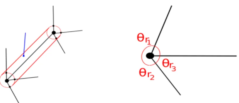
A discrete s-rep is a sampling of this continuous skeletal model. It consists of anm×n grid of samples, calledhubs, from the skeletal surface with either two (on the interior) or three (along the crest) vectors calledspokespointing from the skeleton to the boundary. These crest spokes are an approximation of the actual configuration in continuous models. In the continuous case there is one spoke emanating from every position on the deflated ball mentioned above. This means that there are two spokes for every non-fold skeletal position and one spoke along the fold curve. As you move along the skeleton the lastdistance to the fold region, the spokes begin to swing with infinite velocity as you move around the fold and onto the other side. The triple-spoked hub for discrete s-reps allow represent this by extending the length of the fold spoke back distance to a hub before the swing begins, restricting that lastlength step to be straight.
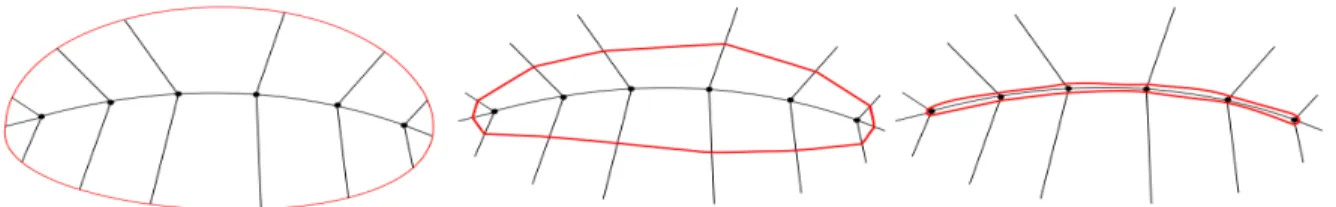
Figure 3.2 shows an example s-rep and the surface implied by varying τ values. The grid structure on the skeleton forms a collection of quadrilaterals with a hub at each corner. It is this discrete representation which must be interpolated back into a continuous model.
Figure 3.2: A 2D s-rep model showing the surface given atτvalues of 1 (left), 0.5 (middle), and 0 (right). The two sides of the surface forτ = 0occupy the same region of space but retain spherical topology. Note that the first and last hubs have 3 spokes, the third being the additional crest spoke which transitions from the top side to the bottom.
3.3 Skeleton Interpolation
As in [50], interpolation of the hubs into a continuous skeleton is done by fitting cubic Hermite patches to the quads of discrete samples which form the surface. This interpolation requires 16 control values: the 4 corner pointsp(u01, u02),p(u11, u02),p(u01, u12),p(u11, u12), the 8 first derivatives of each corner point in both parameter directions which are computed via finite difference approx-imation, and the 4 second order mixed partial derivatives of each corner point, which are set to 0. The matrixHccontaining these control values which will be used to interpolate the skeleton is
Hc =
p(u0
1, u02) p(u11, u02) pu2(u
0
1, u02) pu2(u
1 1, u02)
p(u0
1, u12) p(u11, u12) pu2(u
0
1, u12) pu2(u
1 1, u12)
pu1(u
0
1, u02) pu1(u
1
1, u02) 0 0
pu1(u
0
1, u12) pu1(u
1
1, u12) 0 0
LetH(x)= (H1(x), H2(x), H3(x), H4(x))andH0(x)= (H10(x), H
0
2(x), H
0
3(x), H
0
4(x))where
Hiare the cubic Hermite spline basis functions:
H1(x) = 2x3− 3x2+ 1
H2(x) = −2x3+ 3x2
H3(x) = x3− 2x2+x
andHi0are their derivatives. Computation at a point(u∗1, u∗2)inside a quad is given by
p(u∗1, u∗2) = H(δu1)·Hc·H(δu2)T.
Derivatives of the skeletal surface can be computed by replacing the appropriate set of basis func-tions by their derivatives:
pu1(u
∗
1, u
∗
2) =H
0
(δu1)·Hc·H(δu2)T; pu2(u
∗
1, u
∗
2) =H(δu1)·Hc·H0(δu2)T (3.2)
Figure 3.3 shows the resulting skeleton for a hippocampus s-rep.
Figure 3.3: An s-rep of a hippocampus (left) and the interpolated skeleton (right).
3.4 Spoke Interpolation
We wish to interpolate an unknown spokeS(u∗1, u∗2). If the sampled hubs have integer parame-ter values,(u∗1, u∗2)can be written as
(u∗1, u∗2) = (u01+δu1, u02+δu2); δu1, δu2 ∈[0,1) (3.3)
where(u0
1, u02)is the top left corner of the quad containing the desired value. Figure 3.4 gives an
Figure 3.4: An s-rep quad, with the desired spoke in blue.
I then interpolate the spokeS(u∗1, u∗2)by beginning from the known spokeS(u0
1, u02)and
inte-grating the derivatives ofSfrom(u0
1, u02)to(u
∗
1, u
∗
2). This approach yields the equation
S(u∗1, u∗2) =S(u01, u02) +
(δu1,δu2) I
(0,0)
∂S
∂u1
du1 +
∂S
∂u2
du2
(3.4)
for the desired spoke. This means that, to interpolateS(u∗1, u∗2), I must be able to compute partial derivatives ofS at every point along the path from(u01, u02) to(u∗1, u∗2). These partial derivatives can be written as
Sui =rUui +ruiU. (3.5)
Thus, to computeSui, we must be able to computeUuiandrui at arbitrary positions within a quad.
In s-reps, changes to the spoke lengthrat some point depend on the changes in the skeletonp
and boundaryB. Damon’s compatibility condition [52][53] for skeletal models is given by
−rui =pui ·U+Bui·U, (3.6)
we obtain the expression
Sui =rUui−(pui·U+ (pui+Sui)·U)U=rUui −(2pui+Sui)U
TU
= rUui−2puiU
TU
I+UTU−1
(3.7)
for the partial derivatives of S. This equation allows for the computation of the spoke derivative at any point(u∗1, u∗2)given derivatives of the skeletal surfacepui, which we can compute using the
method described in section 3.3, and the spoke directionUui at that point.
3.5 Estimation of Spoke Direction Derivatives via Quaternion Splines
The partial derivatives of the spoke direction vector fieldUuiare needed to solve equation 3.7.
BecauseUis a unit vector field, changes inUcan be represented as rotations. For this reason, I use a quaternion-based interpolation to compute these derivatives.
Each spoke at the corner of a quad is represented by a quaternion. Each unit vector U = (Ux, Uy, Uz)is represented by the unit quaternionq= 0 +Uxi+Uyj+Uzk. From the four spoke direction quaternions bounding a quad, the spoke directions on the interior of the quad must be interpolated.
A computationally inexpensive method for this interpolation is spherical linear interpolation (slerp) [54] Using slerp, the quaternion that is λ (∈ [0,1]) of the distance between two adjacent quaternionsqiandqi+1is given by
SL(qi,qi+1, λ) =qi(q∗iqi+1)λ. (3.8)
However, as its name suggests, this method would only haveC0continuity across quad boundaries.
For this reason, a higher order method is needed.
Instead of this analogue of linear interpolation, I use an extension of the cubic B´ezier curve to the surface of a sphere called squad[55] to interpolate quaternions in a quad interior. To ensure
must be chosen carefully. For a curve, two of the control points (qi andqi+1) are the two points
between which we are interpolating. The other two points,aiandai+1, are computed by
consider-ing not onlyqi andqi+1 but alsoqi−1 andqi+2 to ensureC1 continuity. The computation forai is thus [55][56]:
ai =qiexp
−log(q
−1
i qi+1) + log(q−i 1qi−1)
4
.
Given these control points, De Casteljau’s algorithm can be used to efficiently compute a B´ezier curve as a sequence of linear interpolations. Given a set of 4 control points, the algorithm proceeds as follows:
1. Connect the control points to form an open polygon with 3 sides.
2. Subdivide each segment into two pieces with length ratiot: (1−t).
3. Connect the points from step 2 to form two line segments.
4. Subdivide the two new segments as in step 2 and connect these points to form a single line.
5. Subdivide this line. The resulting point is on the curve.
Figure 3.5 shows the application of this algorithm to a simple example.
A similar approach allows for computation of squad by leveraging slerp (equation 3.8), giving the quaternion equation
SQ(qi,qi+1,ai,ai+1, λ) =SL(SL(qi,qi+1, λ), SL(ai,ai+1, λ),2λ(1−λ)) (3.9)
Differentiating equation 3.9 with respect toλyields [56]
SQ0(qi,qi+1,ai,ai+1, λ) =
SL(qi,qi+1, λ) log(q∗iqi+1)gi(λ)2λ(1−λ)+SL(qi,qi+1, λ) g0i(λ)
2λ(1−λ)
(3.10)
wheregi(λ) =SL(qi,qi+1, λ)∗SL(si,si+1, λ).
The derivativeUu1(u
∗
1, u∗2) within a quad is computed by first using equation 3.9 to estimate
U(u−11, uδu2
2 ),U(u01, u
δu2
2 ),U(u11, u
δu2
2 ), and U(u21, u
δu2
2 ) via the 4× 4 surrounding grid spokes.
Equation 3.10 on the resulting quaternions then yields the desired derivative. The computation is similar forUu2.
3.6 Interpolation of the Crest
The method described in the previous sections works without modification on quads adjacent only to quads on the same side of the object. However, interpolating quads which go around the crest from the top to the bottom of the object requires special consideration because their geometry differs from that of other quads. The major difference in the s-rep structure at the crest is that adjacent spokes can emanate from the same hub. This yields degenerate quads which are collapsed into lines, causing difficulties in the direct application of equation 3.7.
Figure 3.6: Left: The dilated crest curve with desired spoke in blue. Right: A cross-section of the crest showing the radius-relative dilation.
end point is set back to be on the original crest curve. 3.7 Spoke Computation via Integration of Derivatives
With the pui and Uui values from sections 3.3 and 3.5, we can start from the quad corner
(u0
1, u02)and integrate equation 3.7 numerically. Using Euler’s method for the integration, taking
a step of length h yields S(uh
1, uh2) = S(u01, u02) + h(δu1Su1(u
0
1, u02) +δu2Su2(u
0
1, u02)). From
(uh
1, uh2), we can take another step towards(u∗1, u2∗)and iterate until(u∗1, u∗2)is reached.
An alternative approach which yields better accuracy is to use a more sophisticated predictor-corrector method for the integration. In particular, I use the Adams method, consisting of an Bashforth predictor followed by an Moulton corrector [57]. Because the Adams-Bashforth predictor for computing a valueyi+1 requiresyi, yi−1, yi−2 andyi−3, Euler’s method is
used until enough previous steps have been computed to bootstrap the Adams method. In this formulation, the choice of the origin corner (u0
1, u02) is arbitrary. We can interpolate
S(u∗1, u∗2) using this method starting from any of the four quad corners. I have found that the stability of the interpolations is increased when I interpolate eachS(u∗1, u∗2)from all four corners and compute the final result as a weighted average of the four interpolations, with the weights being the relative distance of(u∗1, u∗2)from each corner.
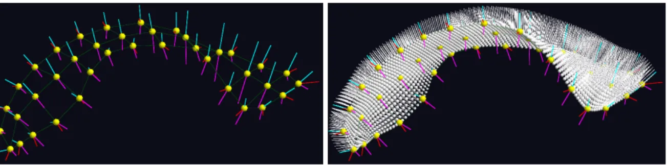
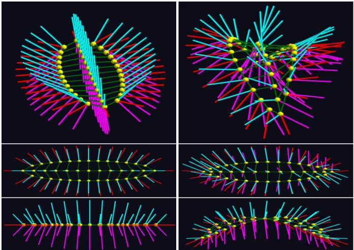
Figure 3.7: A lateral ventricle s-rep and a dense interpolation of its top side spokes.
this method to an s-rep of an ellipsoid where the medial sheet can be computed analytically. In this ellipsoid, interpolated spokes along the top and bottom differ by no more than5◦ from their computed counterparts. Spokes along the crest, particularly in the four corners of the s-rep grid, have higher errors but none more than10◦.
3.8 Discussion
This chapter presents a geometrically-based method for continuously interpolating discrete s-reps. While it is difficult to evaluate my method’s accuracy due to the lack of ground truth values to compare against, it has produced smooth and reasonable surfaces for a variety of anatomical objects, including objects where older m-rep and s-rep interpolation methods failed. Having an accurate interpolation method is useful in a variety of tasks. It makes s-rep fitting more accurate, it can be used to optimize correspondence over a population of s-reps by shifting spokes to interpo-lated positions, transfer labels from one s-rep to another via object-relative coordinates, and it can be used to generate s-rep-relative appearance models such as the one described in chapter 5.
4 PROBABILITY DISTRIBUTION ESTIMATION OF SHAPE DIFFERENCES
4.1 Introduction
A common approach in segmenting a structure from a medical image is to use prior knowledge of the shape of that structure. One way to incorporate this prior knowledge, given a training set of instances of the object, is to estimate the probability distribution of that shape and only choose potential segmentations either directly from this distribution or based on their closeness to it.
In the segmentation problem I am considering in this dissertation, however, I already have specific prior knowledge of the shape of the prostate in a patient’s ultrasound from their planning-time MRI, so I have less need to estimate the possible distribution of all prostate shapes. Rather, I wish to model a distribution which allows for the use of this patient-specific knowledge. Because of this, I choose to model the effect of the transducer-induced deformation on the prostate in order to best leverage the prior knowledge given by the MRI for estimating the prostate shape in TRUS. In order to effectively estimate the probability distribution on these shape differences, careful consideration must be given to the method by which the objects and their differences are analyzed. As discussed in section 2.1, shapes are best thought of as non-linear entities, so typical Euclidean statistical methods such as PCA are ill-suited for direct application to shape data. This is partic-ularly the case with s-reps. Because the space of shapes is curved, the difference between a pair of shapes in the space will be a curve along the manifold, such as a geodesic connecting the two shapes. The problem then becomes estimating a probability distribution of geodesics in this curved space.
of points become line segments which can be analyzed using standard statistical techniques. I apply this method to PDMs in several toy experiments as well as to s-reps fit to clinical prostate data.
I consider this modeling of the difference between pairs of shapes (in this case, the prostate shapes from a single patient’s planning-time MRI and biopsy-time TRUS) as a restricted form of the general problem of longitudinal shape analysis. While the goal of longitudinal analysis is to learn the various ways in which a population of objects change over various time points, I am only concerned with the effect of a specific process on pairs of prostate shapes at a given time pair. However, many of the techniques discussed in this chapter could be applied to a more general longitudinal problem.
4.2 Related Work
Early work on this problem includes the work by Mardia and Walder [58] on so-called paired shape distributions, where they consider two shape distributions with different means and vari-ances but correlation between the two classes. They use maximum likelihood estimation to esti-mate unknown parameters of this correlation and to determine if there are statistically significant differences between the two classes.
I contrast the problem being considered here - statistical analysis of the differences between pairs of objects - with the class of methods where the change between shapes is the base object being considered, such as the methods based on Large Deformation Diffeomorphic Metric Map-ping (LDDMM). There are two general ways in which statistics on such objects is done: either on the full deformation fields themselves or on their initial momentum. Methods in the first cate-gory [59, 60] involve performing PCA on these deformation fields. While not theoretically ideal, these methods often perform adequately well in practice, though they are not guaranteed to yield smooth or invertible transformations.
lie in a tangent space, they provide a linear representation of the non-linear deformation between two shapes so linear statistical methods can be applied.
There is already an established method for analyzing s-reps while taking into account their underlying manifold structure. PNS-based Euclideanization has been shown to produce compact statistics of s-reps (and PDMs) for tasks such as hypothesis testing [10], classification [5], and producing correspondencing objects [6]. For this reason, I choose to study s-rep differences within this framework rather than adapting another approach to work with s-reps directly.
As mentioned, I am only concerned with changes between a starting and ending shape, each of which is at a known time point. This is contrasted with the more general area of longitudinal analysis, where there are often more than two shapes in a sequence and their exact time points relative to the underlying change are unknown. A detailed review of general longitudinal shape analysis methods can be found in [63].
4.3 Methodology
In this section I describe the methodology by which I compute probability distributions on changes of pairs of shapes. The first several sections describe the general analysis methodology which can be applied to various shape representation while the latter sections deal specifically with initialization of s-reps for analysis.
4.3.1 Euclideanization
The first step I take is to convert shape representations which live on manifolds into a form on which more standard Euclidean statistical techniques may be applied. To do this I use princi-pal nested spheres (PNS) as described in section 2.2.3 to compute a polar system (consisting of pole/angle pairs for each subsphere) which can be used to create Euclideanized versions of the input shapes.
ending shapes, or the union of all of the shapes.
I choose to base the PNS calculation on the union of all training shapes for several reasons. First, if the training were based only on one of the two sets of shapes, instances from the other set may be outliers in the estimated shape space and thus have unstable representations (if much of the variation is captured in the low-variance spheres of the PNS computation, for example). Using a larger training set is also advantageous in situations where the amount of training data is limited as is typical in medical applications. This approach is not suited to situations where the expected deformations are very large, however. In such cases, using one class of shapes as the basis for the PNS calculation may be preferable.
4.3.2 Probability Distribution Estimation
Once the PNS polar system has been computed, I subtract the starting shape from the ending shape to get the difference of their Euclideanized values. I then apply PCA to these values to estimate the probability distribution of these differences.
This subtraction can be thought of as a transport, where subtracting the starting shapes from the ending shapes is analogous to transporting each starting shape to a common point and transporting each corresponding ending shape in the same way. If this analysis were performed directly on the curved manifold, the non-trivial problem of how to transport the geodesic connecting two shapes to a common location would have to be addressed. I avoid the problems inherent of transports on general curved spaces by performing this transport in the Euclideanized space.
4.4 Evaluation
First, I evaluate the performance of my proposed approach on a set of ellipsoid boundary PDMs which are deformed by twisting and/or bending. The results of the proposed method are compared to results computed by directly taking pointwise differences between the PDMs in Euclidean space followed by PCA. I then show the result of applying the Euclideanization-based method to ellipsoid s-reps.
and/or twisted following a specific distribution. Each set of ellipsoids has principal radii following Gaussian distributions with means40,20, and15and standard deviations3,2, and1.5respectively. For each group of 100 ellipsoids, a mean bend angle θ and mean twist angleφ are selected. The 100 ellipsoids are then bent and twisted by angles randomly generated from Gaussian distributions with those means, generating the pairs of ellipsoids on which my analysis is done. Deformations are done by first twisting the ellipsoid boundary about the long axis followed by a bending of the long axis.
4.4.1 Single Mode of Change
For ellipsoids with single (either bending or twisting alone) modes of change, both my method and standard PCA were able to identify a single dominant mode of variation. For bending, distribu-tions with means of0andπ/6yield a distribution whose first principal variance accounts for 98%
of the total variance using both methods of analysis. For twisting, a 0 mean distribution yields a similar 98%principal variance for both analyses, while aπ/3mean distribution yields 93%. In all cases, the Euclideanization-based method yields deformations which, when visualized, move more naturally and follow curved paths than using PCA alone, which produces linear deformations.
I also study how well the mean deformation computed by each method recovers the expected bending or twisting angle. To do this, I apply the mean deformation to an undeformed ellipsoid and compare the average angle the points are bent or twisted by to the expected angle. Figure 4.1 shows the results of this experiment. Both methods are able to accurately recover the bending and twisting angles, though the Euclideanization-based method is slightly more accurate.
Figure 4.1: Bending (left) and twisting (right) angles estimated from computed mean deformations compared to ground truth.
Actual Eucl. PCA 30 29.87 28.50 45 43.67 42.73 60 59.67 57.45
4.4.2 Composed Bending and Twisting
Next I consider ellipsoids whose deformations are a combination of a twisting followed by a bending. Both methods are able to separate bending and twisting deformations into separate eigenmodes. However, the estimated principal variances can be very different.
In order to test which method’s estimated principal variances are more accurate, I designed an experiment where the relative size of the bending and twisting variances should be equivalent and compare the results of both methods to the expected results. Because twisting is done about the longest principal radius while bending transforms it, a twist of some angle θ produces less change to the points of the PDM than a bend of the same angle. For a twisting angle of π/3, the parameters for the bending angle distribution are computed to yield approximately the same change to each point’s position (and thus the total variance should be approximately even between the two modes). This scaling is done by using the knowledge that bending is applied in the plane which intersects the ellipsoid in its two largest radii, while twisting is applied in the plane of the two smallest. Once the twisting angle is chosen, a bending angle which will move points on the ellipsoid boundary by the same Euclidean distance as the twisting angle can be computed. For this data, PCA yields two large principal variances which account for 65%and 28% of the total variance. The Euclideanization-based method yields principal variances of49% and46%, which are much closer to the expected values. Furthermore, the dominant mode of the PCA distribution is a bending deformation rather than a twist, even when the angles are adjusted so that the twisting deformation should be slightly larger, showing that PCA tends to overestimate the effect of the bending transformation relative to the twisting.
for each set. The five ellipsoids resulting from the mean PCA deformations have an average MSE of 1.038 from the expected result while the five deformations produced by the Euclideanization-based method have an average MSE of 0.664. Figure 4.2 shows the results for each individual experiment.
Bending 30 45 45 60 60
Twisting 45 45 60 45 60
PCA MSE 0.62 1.13 0.90 1.52 1.02 CPNS MSE 0.31 0.87 0.59 0.71 0.84
Figure 4.2: MSE between the estimated mean deformations of PCA and CPNS compared to the expected mean deformation.
4.4.3 Application to S-reps
This approach of first Euclideanizing a shape representation before then estimating probabil-ity distributions of their differences can also be applied to s-reps. Because the s-rep manifold is a product of various spaces (some spherical and some not), a single PNS can not be used for an entire s-rep. Instead, the various components of the s-rep are Euclideanized separately and these Euclideanized values commensurated and combined into a single vector in a process called compositing. The details of this method are given in section 2.2.4. Differences between these Euclideanized representations can then be computed and their probability distribution can be esti-mated. Figure 4.3 shows the result of applying a computed mean of bending and twisting defor-mations with twisting angleπ/3and bending angleπ/6to an ellipsoid s-rep. Figure 4.4 shows the result of deforming the s-rep along the first two eigenmodes of this deformation, with the first prin-cipal component being mostly twisting and the second mostly bending, showing good separation of the two types of deformation into separate principal components.
4.5 Discussion
Figure 4.3: Three views of an ellipsoid s-rep before (left) and after (right) application of computed mean deformation. As expected, both bending and twisting can be seen in the mean
magnitude of these changes relative to applying PCA directly on PDM differences. When ap-plied to s-reps of deformed ellipsoids, the Euclideanization approach computes a reasonable mean deformation and correctly separates the components of the deformation into separate eigenmodes. This method could be extended to more general longitudinal analysis problems. Once a se-quence of multiple shapes has been Euclideanized, standard techniques such as regression could be used to estimate how shapes are changing over time.
5 MODELING TRUS APPEARANCE VIA REGIONAL TEXTURE CLASSIFIERS
5.1 Introduction
As mentioned previously, deformable model segmentation involves deforming an object rep-resentation so that it better matches the boundary of the desired object in the image. A common approach is to build a statistical model of the appearance of an object in a particular modality and use this model in driving the optimization. Building a single, global model for appearance can be successful when an object’s appearance is relatively uniform or it has strong contrast with the neighboring anatomy. When these properties do not hold, however, a more fine-grained approach is required.
Segmentation of the prostate from TRUS is challenging in part because of the difficulties in discerning the edges of the prostate in ultrasound images. The appearance of both the prostate and its surrounding anatomy varies widely around its boundary, making the use of a single global appearance model insufficient and motivating the use of a locally-defined one. In addition, issues of constrast and noise-like speckle present in the ultrasound images makes direct analysis of ultra-sound intensity unreliable. Instead, we define appearance in a local fashion using derived texture features. S-reps provide a convenient method for defining local boundary patches that correspond across multiple cases. For each patch we take the approach of training a classifier on both texture and intensity to distinguish between the appearance of voxels just inside the prostate boundary in that region from those just outside.
This overall approach shares several similar characteristics with many of the methods discussed in section 2.2.6, but it has several important characteristics which none of the other methods fully capture. Some of the classification-based methods discussed previously perform segmentation based on the binary decisions output by the classifier, while others turn the classifier outputs into continuous values using various methods such as application of a sigmoid function to map outputs to [0,1]. Instead, I use an application of Bayes’ theorem to further leverage the training data in order to better understand what the likely distribution of classifier outputs will be when applied to a new image.
Perhaps the most important characteristic that my method uses for modeling ultrasound ap-pearance is the strong level of localization used in the training of the apap-pearance classifiers. While other methods, most notably those of Zhan et al. [40] and Yang et al. [46] use locally trained classifiers of prostate appearance, they train over many fewer and much larger regions (15 and 6, respectively). This means that their regions often contain many disparate types of tissue and textures which can lead to poorer classification results, particularly if there is tissue which is rel-atively similar to prostate texture. In contrast, I am able to leverage the strong correspondences provided by s-reps to train much more localized texture classifiers, allowing for these classifiers to be more finely tuned for the specific regions of the image in which they will be applied. Be-cause s-reps have been shown to produce stronger correspondence than the PDMs typically used in ASM-based segmentations, these classifiers can be consistently applied on voxels in the correct regions, minimizing the main drawback of such a scheme.
5.2 Materials
5.3 Methodology
In order to build a local appearance model, we must be able to define local regions of the object boundary which correspond across the training cases. Given a set of such regions, the voxels just inside the boundary at a region form one class, while the voxels just outside the boundary make up the other.
For each voxel we have a feature tuplef consisting of some combination of intensity, texture, or other derived features. For each patch we pool together the inside and outside features from each training case to form overall inside and outside classes for that patch. From these two classes we use distance-weighted discrimination (DWD) [64] to compute a separation direction vin feature space which best separates the appearance of voxels inside and outside the prostate boundary.
Given a separation directionv, we project each training pointf ontovyielding a valued. If we consider the threshold on the separation direction to be atd = 0, the sign ofdindicates to which classf has been assigned, while its magnitude is distance from the separating hyperplane and thus indicates confidence in this assignment under the assumption that points further from this hyper-plane are more likely to be correctly classified than those nearer to it. We form two histograms of
dvalues, one for those voxels from inside the boundary and one for voxels outside the boundary. These histograms represent the probability distributionsp(d|in)andp(d|out), respectively.
Given a new feature tuple, such as one from an image to be segmented, we wish to determine whether it is more likely that this feature tuple came from inside or outside of the prostate. Assum-ing we know which regions of the prostate the voxel came from, we can project it along thevfor that region and get itsdvalue. From thisdvalue we wish to knowp(in|d). Using Bayes rule we have
p(in|d) = p(d|in)p(in)
p(d|in)p(in) +p(d|out)(1−p(in))
p(in|d) = p(d|in)
p(d|in) +p(d|out) (5.1)
This allows for the computation of the probability that any particular voxel came from inside the prostate.
5.4 Application
To build a local appearance model, we must first be able to define local regions around the prostate boundary which are in correspondence across the training cases. The s-rep fitting pro-cess ensures that each prostate’s s-rep comes from the same shape space and produces reasonable correspondence across cases.
Given a set of fit s-reps, we define a local boundary region to be centered at the end of a spoke and extend halfway to neighboring spokes in each direction, forming a quadrilateral on the boundary. By moving some distance along the spoke in either direction, we can form inside and outside regions for the voxels near the boundary.
5.4.1 Ultrasound Appearance Model
As a preprocessing step, each of the TRUS images isunfannedso that the insonation direction, the direction along which the sound propogates, runs along one of the major axes while the others represent two axes orthogonal to it. This is done under the observation that much of the texture information happens either along or orthogonal to the insonation direction. Figure 5.1 shows an example of the original ultrasound and its unfanned counterpart. In order to decrease the variance in the ultrasound intensity and to better separate texture and intensity, we run speckle-reducing anisotropic diffusion [21] on each image. This produces a smoothed intensity image. The differ-ence between the original image and the smoothed one yields a texture image upon which we can do texture-based analysis. Figure 5.2 shows an ultrasound image along with its derived intensity and texture images.
Figure 5.1: An original, fanned ultrasound
on the left and its defanning on the right. Figure 5.2: The unfanned ultrasound on theleft, despeckled intensity image in the mid-dle, and texture image on the right.
method. As noted in section 2.2.6, previous work has been done on ultrasound prostate segmenta-tion making use of either 2D or 3D Gabor filters, and this is what we choose to use here. At each voxel in the image, we compute 2D Gabor features in 6 orientations, 2 scales (5 and 10 voxels), and 2 phases in each of the 2 orthogonal planes which include the insonation direction. Combining these 48 values together with the voxel’s intensity yields a 49-dimensional feature tuple for anal-ysis. In chapter 6 I show how these feature tuples, after being converted into probabilities, can be used to drive the image match term of a deformable-model based segmentation.
5.5 Evaluation
Here I evaluate the effectiveness of the appearance model specifically in how well the local classifiers can classify inside from outside without regard to its ultimate application of segmenta-tion, which will be discussed in chapter 6.5.