Two essays on life cycle models

Daver

_{Cuneyt Kahvecioglu}

A dissertation submitted to the faculty of the University of North Carolina at Chapel Hill

in partial fulfillment of the requirements for the degree of Doctor of Philosophy in the

Department of Economics

Chapel Hill

2006

Approved by

Advisor: David Blau

Reader: Tom Mroz

Reader: Donna Gilleskie



₂₀₀₆

Daver Cuneyt Kahvecioglu

DAVER CUNEYT KAHVECIOGLU:

Two Essays on Life Cycle Models

(Under the direction of David Blau)

This dissertation consists of two essays. In “A Life-Cycle Model: Retirement, Savings, and Portfolio

Allocation”, I analyze the interrelationships among retirement, saving, and asset allocation. I show that optimal

portfolio allocation can be very sensitive to plans about retirement timing and to the presence and characteristics

of Social Security. I also show how portfolio decisions have impact on when to retire. In order to take into

account these important effects, Social Security reform proposals should be evaluated with models that

incorporate portfolio choice.

In the second essay, “Asset Allocation, Bequests, and Wealth Dynamics of the Elderly”, I build and estimate a

life cycle model of asset allocation and saving with a fixed cost of stock market entry, medical expenditure risk,

and a general bequest function that captures risk preferences over bequests. The estimates imply that there is no

operative bequest motive, and that medical expenditure risk is a very strong motivation for saving at older ages.

Even though the model explains reasonably well both the observed average age profiles and the heterogeneity in

saving and portfolio allocation, the cross-equation restrictions that are required for internal consistency are

strongly rejected. This is mainly due to the fact that, in constant relative risk aversion utility, a single parameter

- coefficient of relative risk aversion - governs both wealth and portfolio paths. While a very high level of risk

aversion is required to explain portfolio choices, a very low level of risk aversion is required to explain wealth

dynamics. Despite its internal inconsistency, the model is one of the richest versions of the standard model and I

use the estimates to do some policy simulations with caution. I used the estimates to simulate the impact of

reducing the Social Security benefit of a 70-year old female retiree by a specific amount, and giving her a lump

sum equal to the expected present discounted value of the benefit cut, which is to be invested in her individual

account. I find that this reform would be undesirable. Main reason behind this is that, most retirees are either

To mom and dad, Melahat and Sabri Kahvecioglu...

I have been very lucky to be around some excellent faculty at the University of North Carolina. I am indebted to

David Blau for his encouragement and excellent guidance and advice. I have also benefited tremendously from

discussions with Wilbert van der Klaauw over the years. For helpful comments and discussions, I thank Donna

Gilleskie, Tom Mroz, Helen Tauchen, and Eric Renault. Ron Gallant provided crucial help on the estimation

technique whenever I needed. Mike Hurd has been very helpful in refining my dissertation topic.

I would also like to express my appreciation to Information Technology Services of UNC for maintaining and

administering UNC’s excellent high-performance computing infrastructure. I especially want to thank Shubin

List of Figures...ix

Chapter I: A Life Cycle Model: Retirement, Savings, and Portfolio Allocation...1

1 Introduction...2

2 Literature Review... 3

3 Theoretical Model...6

3.1 Solving the Model...10

4 Simulations... 14

4.1 Simulations without Social Security...16

4.1.1 Retirement...18

4.1.2 Consumption and Assets...20

4.1.3 Portfolio Allocation... 21

4.1.4 Behavior of Groups of Various Retirement Ages...22

4.2 Simulations with Social Security... 27

5 Analyzing the Solution in More Detail... 29

6 Conclusion... 42

Chapter II: Asset Allocation, Bequests, and Wealth Dynamics of the Elderly... 43

1 Introduction...44

2 The Model... 48

2.1 For Retirees Who Have Already Paid the Entry Cost...48

2.2 For Retirees Who Have Not Paid the Entry Cost... 50

2.3 Preferences and Asset Returns...51

2.4 Out-of-Pocket Medical Expenditure... 52

4 Data... 57

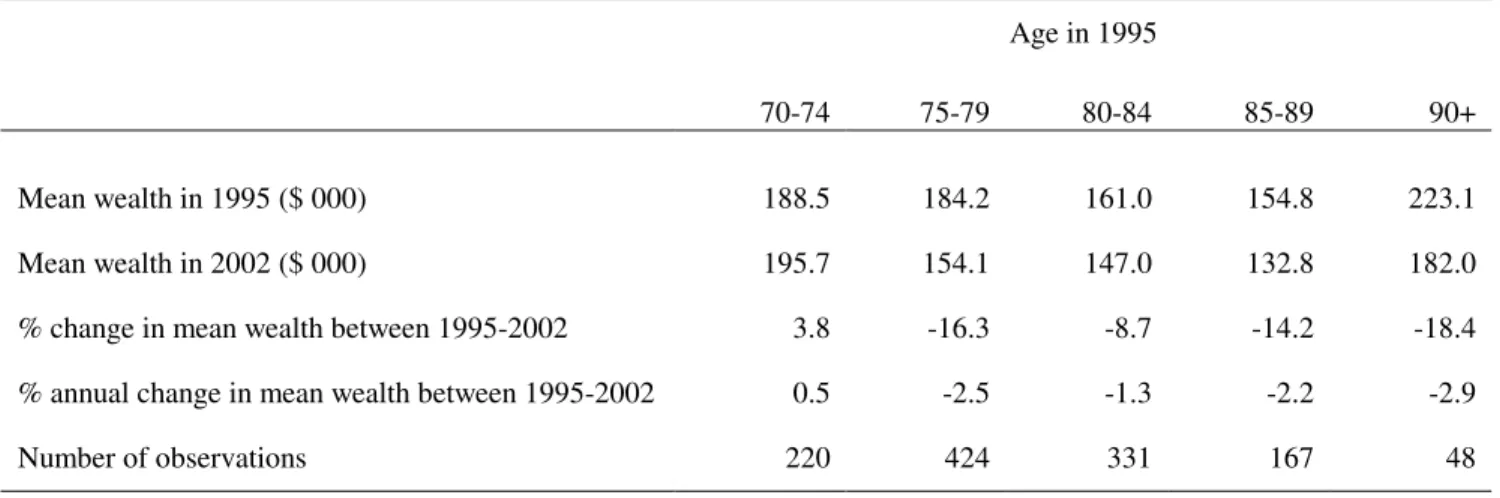
4.1 Are the Assets of the Elderly “Melting Down”?... 59

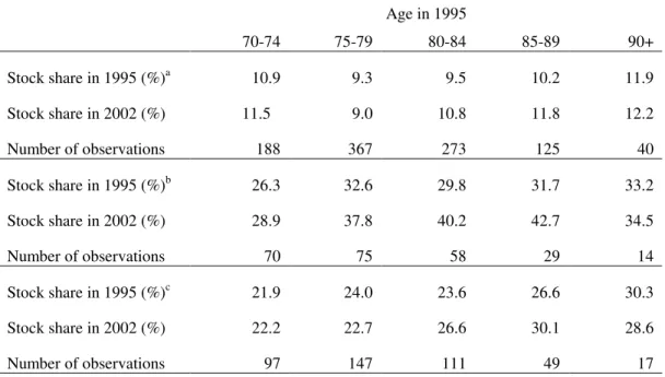
4.2 How Do the Stock Shares Vary with Age?...60

4.3 Stock Returns... 61

5 Estimation... 62

5.1 Prorating Predicted Variables... 65

6 Results...66

6.1 Risk Aversion and Discount Factor... 66

6.2 Fixed Stock Market Entry Cost... 69

6.3 Is There A Bequest Motive?... 70

6.4 Behavioral Implications of Medical Expenditure... 71

6.5 Model's Fit... 72

6.6 Policy Simulations... 73

6.1.1 No Access to the Private Annuity Market... 74

6.1.2 Private Annuity Market Is Available... 76

7 Conclusions...76

Appendix...97

Table 1 How the Simulation Is Done...16

Table 2 Timing of Retirement without Social Security... 19

Table 3 Timing of Retirement with Social Security... 27

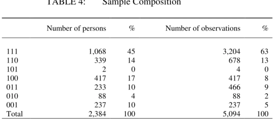
Table 4 Sample Composition...79

Table 5 Selected Averages for Successive Panels of the AHEAD Data... 79

Table 6 Change in Mean Wealth by Age between 1995 and 2002...80

Table 7 Change in Median Wealth by Age between 1995 and 2002...80

Table 8 Change in Mean Stock Share by Age between 1995 and 2002... 81

Table 9 S&P500 Returns over the Interview Years...81

Table 10 Estimates of the Structural Parameters... 82

Table 11 Welfare Effects of the Social Security Reform on a 70-Year Old Female Retiree Who Has the Median, Mean, and the 90th _{Percentile Wealth and Income of the Sample... 83}

Table 12 Probabilities of Being in the Low, Medium, and High Expenditure Categories... 97

Figure 1 Employment Rate by Age... 19

Figure 2 Average Consumption, Income, and Assets by Age... 20

Figure 3 Average Portfolio Allocation by Age...22

Figure 4 Average Consumption by Age by Groups of Various Retirement Ages... 24

Figure 5 Average Wealth by Age by Groups of Various Retirement Ages...25

Figure 6 Average Incomes by Age by Groups of Various Retirement Ages... 25

Figure 7 Average Returns on Risky Asset Holdings by Age by Groups of Various Retirement Ages...26

Figure 8 Average Portfolio Allocation by Age by Groups of Various Retirement Ages... 26

Figure 9 Average Consumption and Assets by Age with and without Social Security...28

Figure 10 Average Portfolio Allocation by Age with and without Social Security... 29

Figure 11 9th _{Period Consumption and Value Function vs Cash-on-Hand... 30}

Figure 12 9th _{Period Consumption and Portfolio Allocation vs Cash-on-Hand... 30}

Figure 13 8th _{Period Consumption and Portfolio Allocation... 31}

Figure 14 7th _{Period Consumption and Portfolio Allocation... 31}

Figure 15 Probability of Next Period Employment vs Cash-on-Hand in Period 9...36

Figure 16 Probability of Next Period Employment at t=9 vs Possible Values of Consumption and Portfolio Allocation... 37

Figure 17 t=9 Value Function as a Function of C and X... 38

Figure 18 Portfolio Allocation vs Cash-on-Hand for Selected Periods... 41

Figure 19 Wealth & Portfolio Trajectories for Various Levels of Risk Aversion when There Are No Bequests... 84

Figure 20 Wealth & Portfolio Trajectories for Various Levels of Risk Aversion toward Bequests (The Level of Risk Aversion for Consumption is fixed at 4)... 84

Figure 21 The Variation in S&P Returns Caused by Having Different Interview Dates for a Given Individual and a Given Wave... 85

Figure 22 AHEAD Field Periods vs. S&P500 Index...85

Figure 23 The Simulated Impact of Bequests for the "Median" Retiree Who Has Already Paid the Stock Market Entry Cost...85

Figure 26 The Simulated Impact of Bequests for the "Median" Retiree Who Has Already Paid the Stock Market Entry Cost...87

Figure 27 The Simulated Impact of Bequests for the "Mean" Retiree Who Has Already Paid the Stock

Market Entry Cost...87

Figure 28 The Simulated Impact of Bequests for the "Wealthy" Retiree Who Has Already Paid the Stock Market Entry Cost...88

Figure 29 The Simulated Impact of Medical Expenses for the "Median" Retiree Who Has Already Paid

the Stock Market Entry Cost...88

Figure 30 The Simulated Impact of Medical Expenses for the "Mean" Retiree Who Has Already Paid

the Stock Market Entry Cost...89

Figure 31 The Simulated Impact of Medical Expenses for the "Wealthy" Retiree Who Has Already Paid the Stock Market Entry Cost...89

Figure 32 The Simulated Impact of Medical Expenses for the "Poor" Retiree Who Has Already Paid

the Stock Market Entry Cost...90

Figure 33 Predicted vs. Actual Mean and Median Wealth for the Estimation Sample by YEAR, AGE,

AND INCOME... 91

Figure 34 Predicted vs. Actual Mean Stock Share for the Estimation Sample by YEAR, AGE,

AND INCOME... 92

Figure 35 Forecasted vs. Actual Mean and Median Wealth for Out-of-Sample Males by

INTERVIEW YEAR, AGE, AND, INCOME...93

Figure 36 Forecasted vs. Actual Mean Stock Share for Out-of-Sample Males by INTERVIEW YEAR,

AGE, AND, INCOME...94

Figure 37 Comparison of the Distributions of Predicted and Actual Conditional Stock Shares... 95

Figure 38 Simulated Impact of the Social Security Reform on the "Median" Retiree Who Has Already

Paid the Entry Cost... 95

Figure 39 Simulated Impact of the Social Security Reform on the "Mean" Retiree Who Has Already

Paid the Entry Cost... 96

Figure 40 Simulated Impact of the Social Security Reform on the "Wealthy" Retiree Who Has Already

1. Introduction

There is a large and growing literature in finance on life-cycle household portfolio allocation. Even

though this literature1 recently acknowledges that labor income may have a big role to play, it ignores the fact

that retirement is a choice and treats it as given. On the other hand, in the economics literature, the portfolio mix

has been treated as given or has been ignored altogether in the models of labor supply and retirement behavior.2

In this paper, I analyze the interrelationships among retirement behavior, savings, and portfolio mix by

modeling these decisions as being made jointly. In particular, I am interested in how the optimal patterns of

life-cycle portfolio allocation are affected by introducing retirement as a choice variable. That information will help

assess the validity of asset allocation advice provided by portfolio managers to the people who are saving for

retirement. Another interesting question that I will explore is whether and to what extent the presence and

characteristics of Social Security affect optimal household portfolio allocations. This is quite important in view

of the current debate about incorporating individual accounts into Social Security. The model proposed in this

paper could be used to analyze the impact of a Social Security reform that introduces individual accounts, while

models that treat the timing of retirement or asset allocation as given would be poorly suited for such an

analysis. Predicting baby boomers' portfolio allocations will also be helpful in forecasting the future trends in

the stock market since they will be holding a significant amount of national wealth.

I have solved and simulated a relatively simple version of the model. I find similar results to the

previous literature when I consider retirement as given. However, if retirement is a choice, I demonstrate that

the model predicts richer and different life-cycle patterns. It is shown that the optimal portfolio allocation can be

very sensitive to expectations about the timing of retirement. Additionally, I show that the presence and

characteristics of Social Security can be very influential on optimal portfolio allocations as well.

1_{Gomes and Michaelides, 2003; Bertaut and Haliassos, 1997; Cocco, Gomes, and Maenhout, 2001; Svensson 1988; Viceira}

2001; Vissing-Jorgensen 1999 to name a few.

2

The rest of the paper is as follows: In section 2, I review the previous work done on the household

life-cycle portfolio allocation. The theoretical model is described in section 3. Model’s solution and its implications

are presented and discussed in the same section. Section 4 concludes.

2. Literature Review

I summarize the relevant literature below. Note that none of the papers discussed here treats retirement,

savings, and portfolio choice as decisions being made jointly.

Addressing the problem of portfolio choice over the life-cycle dates back to the seminal papers,

Samuelson (1969) and Merton (1969). They showed that optimal portfolio allocation is independent of both age

and wealth. The agents in their model should hold a positive fraction of their wealth in risky assets and this ratio

is fixed over the lifetime and over the level of wealth. It is now known that this result is sensitive to the papers'

assumptions (some of them were implicitly assumed in the papers). As explained in Ameriks and Zeldes (2001),

among those assumptions are: (1) asset returns are independently and identically distributed over time, (2)

households have utility functions that exhibit constant relative risk aversion (CRRA) and that are time-invariant

and additively separable over time, (3) markets are frictionless and complete.

There was no labor income in Samuelson's (1969) model. However, without violating any of the above

3 assumptions Merton (1971) adds a labor income process to the model and the qualitative results do not

change. Introduction of labor income to portfolio choice models was somewhat trivial if the following two

conditions are satisfied as in Merton (1971): 1) Labor income is treated as income from traded3 human wealth,

that is investors are allowed to borrow against their human capital. 2) Human wealth is assumed to be nontraded

but traded assets provide perfect hedges against labor income. In other words, investors are able to fully insure

3

their labor income risk. Note that labor supply was not endogenous in Merton (1971). Bodie, Merton and

Samuelson (1991) extend that model by including leisure as a second good and hence endogenizing labor

supply, but they assume that retirement occurs at a fixed age and that households can borrow against their future

labor income. As I will explain below, both of these assumptions are dropped in this dissertation since they are

unrealistic. They focus only on the relationship between labor supply flexibility and portfolio choice.4 They find

that flexibility of labor supply leads to higher shares of the risky asset in the optimal portfolio allocation.

The more recent articles solve for optimal portfolio allocation patterns with at least one of those

assumptions relaxed. Some articles assess whether the observed household behavior is attributable to the more

realistic models. Cocco, Gomez and Maenhout (2001) points out that many households cannot capitalize future

labor income and hence face borrowing constraints due to moral hazard issues. Moreover, they also face

uninsurable labor income risk since explicit insurance markets for labor income risk are not well-developed.

The authors consider a finitely-lived investor facing mortality risk, borrowing and short-sale constraints, and

receiving labor income. The agent can invest in a risky asset or a riskless asset. Using the PSID they estimate

the labor income profile and its risk characteristics and then calibrate and solve numerically for the optimal

portfolio and savings decisions. Stock returns are allowed to be correlated with labor income shocks. They find

that the optimal share of stocks in the portfolio goes down as agents age and as wealth increases, in contrast to

the findings of Samuelson and Merton. This is very similar to my model except in my model retirement is

endogenous. I will show that if I take retirement as given then I obtain similar results as theirs, but treating

retirement as a choice variable changes the monotonicity of the share of risky assets with respect to wealth and

age.

Ameriks and Zeldes (2001) examine the empirical relationship between age and portfolio choice using

new panel data from TIAA-CREF and pooled cross-sectional data from the Surveys of Consumer Finances.

They document significant non-stockownership, wide-ranging heterogeneity in allocation choices, and the

infrequency of active portfolio allocation changes.

4_{They propose that labor supply flexibility can be measured by the number of adults in the household, or having an}

Most of the rest of the literature describing and analyzing the dependency of portfolio allocation on age

has a common motivation: Solving the micro-level equity premium puzzle. There are patterns in data that are

inconsistent with portfolio theory: There is a very sizable fraction of the U.S. population5 that does not hold any

equities. Papers in this literature have added uninsurable labor income (which may or may not be correlated

with asset returns), permanent and temporary wage shocks, non i.i.d. asset returns, borrowing constraints, short

selling constraints, fixed costs for stock market entry, transaction costs for stock trading, and others in attempts

to try to solve the puzzle.

Using data from the PSID and other data sets Vissing-Jorgensen (2002) estimates a dynamic panel data

model of stock market participation and equity share in portfolios controlling for unobserved heterogeneity and

the endogeneity of initial conditions. She focuses on the effects of the first and second moments of

non-financial income and costs of stock market participation on stock market participation and on equity shares in

household portfolios. She finds that both of them contribute to the explanation of the puzzle. She finds evidence

of a positive effect of mean non-financial income on the probability of stock market participation and on the

proportion of wealth invested in stocks conditional on being a participant. Variance of non-financial income is

found to have the opposite effect on those two variables. She also finds evidence of state dependence in the

stock market participation decision, a result that is consistent with the theory that small fixed costs for stock

market entry may deter stockholding. In her study, labor income is treated as given.

Haliassos and Michaelides (2001) show that the puzzle is robust to relaxations of the benchmark

assumptions of Samuelson (1969). They find that assuming that there is a relatively small fixed costs for stock

market participation may help explain the puzzle. They state that such costs can arise from informational

considerations, sign-up fees, and investor inertia.

The timing of retirement, and thus, to some extent, labor income is not given. Households may adjust

their labor supply as events unfold over the life-cycle. Social insurance programs such as Social Security,

5

Disability Insurance, Medicaid, Medicare and the others have the potential to influence savings, retirement

timing, and portfolio choice behavior because they affect the riskiness and amount of current and future income.

Hence it is crucial to model these three decisions jointly. As I will demonstrate in the next section, optimal

portfolio allocation can be very sensitive to plans about retirement timing and to the presence and characteristics

of the Social Security.

3. Theoretical Model

The agent in the model has a finite horizon, T with discrete time t = 1,...,T. Each period corresponds to

one year. The agent dies at T+1 with certainty and there is no risk of death prior to T+1. There is no bequest

motive. Suppose T is 10.

There are three decision variables: Employment, consumption/saving, and portfolio allocation. There is

one risk-free, and one risky asset over which the portfolio decision is made. Wage offers and portfolio returns

are stochastic.

At the beginning of each period, the agent observes the return shock that applies to his assets carried

over from the previous period and so determines his beginning-of-period assets. At the same time he observes

the wage offer for current period employment. He then decides whether to be employed or not, how much to

consume, and if he decides to hold financial assets, what the portfolio allocation is. Note that I do not consider

the hours of work decision. Since there is one risky and one risk-free asset, I define his portfolio decision to be

simply the ratio of his financial wealth held in the risky asset to his total financial wealth.

Choice Variable 1: Employment







t period in employed not

0

t period in employed

1

Choice Variable 2: Consumption

*

t

A

t

I

t

A

t

C

=

+

−

and

A

*

_t

Choice Variable 3: Portfolio Allocation

In the following definition, xt is the fraction of financial wealth held in the risky asset. That is a measure of the

riskiness of the portfolio.

* t A t Z t M t Z t Z t x = + =

where Zt = xt At* is the amount of risky asset held and Mt = (1-xt)At* is the amount of risk-free asset held.

RETURNS:

*

1

-t

A

t

R

]

1

-t

x

t

z

)

1

-t

x

(1

t

[r

t

A

4

4

4

4

3

4

4

4

4

2

1

−

+

=

The returns on the risky asset (z) and on the risk-free asset (r) are realized at the beginning of the next period.

θ

t

z

t

z

=

+

2

)

θ

σ

i.i.d.N(0,

~

t

θ

For simplicity, I assume that return shocks and wage shocks are uncorrelated.

INCOME:

If the agent works, he earns labor income that depends on experience. If the agent does not work, he

may be eligible for pension payments that depend on his labor market experience. In the current model, an agent

cannot collect benefits and work simultaneously. Hence income is

t

)B

t

j

(1

t

W

t

j

t

I

=

+

−

where labor income is

W

_t

=

β

₀

+

β

₁

e

_t

+

η

_t

t, and ηt ~ i.i.d. N(0,ση2).

Social Security/Pension Income is deterministic and collected only if not employed:

t)

,

t

B(e

t

B

=

In the simulations, I set B(e,t) = 0 for e<6; B(6,t) = 5, B(7,t) = 10, B(8,t) = 12, and B(9,t) = 15.

Benefits are in $000’s. Note that this schedule is a crude approximation to the Social Security benefit rules by

requiring a minimum number of work periods for any benefit, providing a relatively low benefit for early

retirement (t = 7, e = 6), and increasing benefits with experience beyond the experience required for normal

retirement (t=8, e=7). Social Security taxes are not modeled.

There is a consumption floor

C

C

if

A

_t

+

I

_t

<

C

0

*

t

A

C

t

C

=

=

Hubbard, Skinner, Zeldes (1995) show that the presence of means-tested social insurance policies

designed to maintain consumption has a large negative effect on saving for lower-lifetime-income groups.

CONSTRAINTS:

x in [0,1]: no short-selling of the risky asset; no borrowing

⇒ Z ≥ 0, and M ≥ 0.

where Z is the amount of the risky asset and M is the amount of the risk-free asset.

A in the above equations is a given constant. I used A = 0 in my simulations, hence I assume that

individuals start period 1 with no assets.

UTILITY FUNCTION: t 1 0 α 1 jt

jt

(γ

γ

t)j

α

1

C

U

+

+

−

=

−

CRRA with parameter α

Most of the studies use CRRA utility functions including the seminal article of Samuelson in 1969.

Choosing the same type of function facilitates the comparison of my results to the other results documented in

the literature.

C

I

A

For

+

≥

For

A

+

I

<

C

Being employed gives a negative utility to the agent (γ0 < 0), which increases with age (γ1 < 0). Dislike

for work is the reason agents retire in this model. Inclusion of disutility of work provides a motive for the agents

to save: saving for retirement. At some point in time they will choose not to work anymore because of the

disutility of working, and they will save for retirement since they are forward-looking. They will also save some

amount due to precaution and intertemporal substitution.

The utility function is additively separable in utility from consumption and leisure. It is straightforward

to modify the function so that it becomes non-separable.

Agents maximize the expected present discounted value of lifetime utility by choosing j (employment),

C (consumption), and x (portfolio mix) at each period t from 1 to T. They discount the future with the discount

factor δ.

3.1. Solving the Model

The model is solved by backward recursion starting from the last period, T. Since there is no analytic

solution of the model I solve it numerically. There are 3 state variables: t (age), et (beginning-of-period

experience), and COHt (beginning-of-period cash-on-hand). Cash-on-hand is defined as assets plus income

(either labor or non-labor). If both of them were serially correlated, then we would have to have 2 additional

state variables: the wage shock and return shock. As a special case, I also solve the model assuming that there is

no Social Security and that wages do not depend on experience. Then, experience is no longer a state variable.

Starting in period T, going backwards to period 1, the model must be solved at every point in the state

space, that is, for every feasible combination of t, e, COH, and j6. However, since COH is a continuous variable,

6_{Note that, actually, j is not a state variable, yet it is treated as if it is one. That is done to save computation time. Instead of}

looping over beginning-of-period assets and labor income, I only loop over cash-on-hand. The downside is that I have to

I discretize it as COH[n], n = 1,...,N. I partitioned the interval of feasible cash-on-hand into 200 subintervals.

The lower end point of the interval is 0. To calculate the other end point of the grid, I calculate the maximum

possible cash-on-hand. I find this number by assuming that the agent receives the highest wage shock (out of

10,000 draws) at current and all previous periods, then saves it all in the form of risky assets and gets the

highest possible return (out of 10,000 draws) in the current and all previous periods. Then I divide this range

into 200 intervals that are smaller towards the lower end but get larger towards the upper end.

It is very unlikely that the agents will have cash-on-hand that is close to the maximum possible one. Hence the

grid is set in such a way that there are more intervals close to the left end point, 0, that is, the grid is coarser

toward the end. Whenever I need to calculate the value of a variable (for example, value function) at some COH

value, which is not at one of COH grid points, I use interpolation.

Period T:

In the last period, the model is solved at every point in the state space (that is, for all feasible

combinations of t, e, n, and j). Since there is no bequest and the agent is going to die at the end of this period

with certainty, there is neither a savings nor portfolio decision to make. Optimal consumption equals

cash-on-hand.

Period T-1:

For each e, n, and j we calculate the consumption and portfolio mix that maximizes the value function:

)]}

(

max

[

)

(

{

max

)

,

(

] 1 , 0 [ ] , 0 [ 1 1 1 1 1 1 1 T j T j T T j T x I A C j

T

e

n

U

C

E

U

C

V

=

+

δ

}

,

max{

A

I

C

C

_T

=

_T

+

_T

A

=

[

r

(

1

−

x

)

+

z

x

]

A

T

T

T

T

T

j

W

j

B

I

=

+

(

1

−

)

A

_T

*

₋

₁

=

A

_T

₋

₁

+

I

_T

₋

₁

−

C

_T

₋

₁

The last term in the above optimization expression is the discounted expected value of last period value

function in T-1. It is,

θ

η

θ

η

d

d

f

V

V

E

V

E

_T

j

_T

_T

j

j

T

j

T

T

T

T T

T

∫∫

=

=

₋

−

1

1

max

max

{

}

(

,

)

where f(.,.) is a joint probability density function. This integral is evaluated using monte carlo simulation.

T

j

T

V

Once those decisions are made, we know the value of end-of-period assets that is carried over to period T. Then

for a number of random draws from the distributions of wage and return shocks, we can calculate the amount

available for consumption. Since agents consume all cash-on-hand in period T, we calculate the period-T-value

function by plugging cash-on-hand in place of C. Averaging over all of the random draws of shocks, we obtain

an approximation of the expected value of the period-T-value function. As the number of draws increases, the

approximation converges to the true value.

The above algorithm is applied for an equally partitioned two-dimensional grid of consumption and

portfolio mix values. 7 Then we search for the pair for which the T-1 value function is maximized. Hence, we

obtain optimal consumption and portfolio decisions for each point in (eT-1 ,nT-1 ,jT-1 ) space. I also calculate the

percentage saved (variable sper) out of cash-on-hand using the consumption values. The variable sper will be

7

used in order to interpolate for consumption during simulation. The results are saved to be used in period T-2

calculations and in simulations.

Although in similar studies the number of draws used in evaluating integrals is less than 100, I used

10,000 draws. Particularly, the portfolio decision is very sensitive to the number of draws used. There were

substantial differences between the portfolio allocation solutions (not consumption or employment solutions)

when I used 100, 1,000, or 10,000 draws.

Periods T-k, k = 2, … ,T-1:

As in period T-1, for each e, n, and j we calculate the consumption and portfolio mix that maximizes

the value function:

)]}

1

(

1

1

1

max

[

)

(

{

]

1

,

0

[

]

,

0

[

max

)

,

(

₋

−

₊

+

₋

₊

+

−

−

+

−

−

−

∈

−

−

+

−

∈

−

=

−

−

T

k

C

T

k

j

k

T

V

k

T

j

k

T

E

k

T

C

k

j

k

T

U

k

T

x

k

T

I

k

T

A

k

T

C

n

e

k

T

j

k

T

V

δ

In contrast to value function calculations in T-1, for periods T-k, k>1, we do not readily know what the

next period optimal choices are given current period optimal choices. In period T-1, next period is the last

period, and we already know that optimal consumption is all of cash-on-hand and there is no portfolio allocation

decision. In periods T-2 and earlier, however, we do not know the next period optimal decision for all the

possible current period decisions. We have calculated and saved only a grid of them. We use an interpolation

algorithm to find the values that are not on the grid points but somewhere in between. For the value function

(especially for power utility functions), an interpolation algorithm based on weighted geometric mean proves to

be “accurate”. For given trial values of consumption and X in T-k, I first find the cash-on-hand available in the

next period. Then find the subinterval that includes this value. Then I interpolate for the value of the value

function at this point by using the already calculated and saved function values at the end points of this interval.

I have tried a number of interpolation algorithms, and found out that this is most appropriate. This method is

better than interpolation based on weighted arithmetic means because for power utility functions it can be

shown that the absolute error for weighted geometric mean is always smaller than the one for weighted

arithmetic mean. I have tried all the interpolation routines in the IMSL package and found out that none of them

are “true” enough to the shape of this kind of utility function.

4. Simulations

Simulation of the solution of the model will be useful to get a sense of what kind of behavior the

agents exhibit during their life courses. Analyzing the solution at each period separately will of course reveal

the most amount of information about the model, but this is more tedious. So I left analyzing the solution to the

next section. In this section, I only focus on the simulation of the solution keeping in mind that we get a limited

insight into the model but a good overview of the model. I present 2 sets of simulation results: One without

Social Security and one with Social Security. In the simulations, I tried to choose all the parameters in a way

such that we have a chance to observe the roles played by the main features of the model.

Using the solution that is described above, the model is simulated for 10,000 agents who are identical

at the beginning of the first period. I describe and explain the solution path for the decision variables over the

life cycle.

During simulation, for the values of state variables that fall somewhere in between the grid points that

were used in the solution, appropriate interpolation methods are used. First, given the beginning-of-period

assets, return shock, and wage offer, cash-on-hand is calculated for both for employment and non-employment.

Value functions are calculated for both values of employment. I use the same weighted geometric average

interpolation algorithm that I used in the solution. Then, the employment value that gives a higher value to the

optimal sper, i.e. percentage saved out of cash-on-hand) and portfolio decisions were calculated for the grid of

all feasible cash-on-hand values. The sper value corresponding to the closest point on the cash-on-hand grid is

the interpolated sper. As will be explained later, true sper may display “jumps” at some cash-on-hand values.

Those jumps are important (they are presented and explained below) and by interpolating sper using the simple

scheme described above we preserve the jumps. Had I used a weighted average of the 2 closest points, I may

have undermined the size of the jumps. We do not need to worry about the size of the error this method causes

because sper is smooth except at those “jump” points, I use a fine grid, and using percentages instead of values

already has a smoothing effect. Given sper, we calculate optimal consumption. To find the interpolated

portfolio mix, we find the portfolio mix value corresponding to the closest point on the cash-on-hand grid. That

value is assigned as the optimal portfolio mix. The same method is applied in calculating the probabilities of

future employment sequences.

Table 1: How the Simulation Is Done

Starting Values:

A

= A

x

= x

e

= 0

Starting values are given. In my simulations A0

*

=0 and x0=0.5

For each t

_θ

η

Rate of return shock and wage offer shock are drawn

z

=



z

+

θ

R

= r

(1-x

) + z

x

W

=

β

+

β

e

+

η

Rate of return on the risky asset is determined

Overall portfolio rate of return is calculated

Wage offer is calculated

For

each

j

(employment status)

I

=W

j

+B(e

,t)(1-j

)

COH

= A

+ I

V

(COH

)

Income and

Cash-on-hand are determined

Value function values are interpolated using the results saved from solution

1 if V

≥

V

j

=

0 otherwise

Employment Status is determined

sper(COH

)

x

(COH

)

A

=sper . COH

C

= (1 - sper).COH

Percentage saved (sper) and

portfolio allocation (xt)

are interpolated using the results saved from solution

End-of-period asset,

Consumption are determined

4.1. Simulations without Social Security

Horizon: T = 10

Constant relative risk aversion parameter: α = 4

Consumption floor: C = 1 (this is set to a very small value in order to concentrate on understanding how the

model works without the complication that the consumption floor introduces.)

Wage function: β0 = 20, β1 = 0, ση= 1 (Average wage is $20,000, wages do not depend on experience, and the

standard deviation of wages is $1,000. I am modeling the decisions of 50+ year olds and since their

wage-experience profile should be relatively flat β1=0 is not a bad assumption. Besides, I get rid of one state variable

(experience) in the case where there is no social security since nothing depends on experience.)

Disutility of work: γ0 = -0.0004, γ1 = -0.00002 (These values are selected to be able to see realistic life-cycle

patterns among the agents. If these were too high in absolute value, then the agent would work only if he

receives an unrealistically big wage shock. In this case almost of them will be on welfare. On the other hand, if

these were too low in absolute value then almost all of the agents would work all the time.)

Risky asset returns: z = 1.04, σ_θ= 0.2 (hence, most of the time: z is in [0.54,1.54]. There were a total of

100,000 draws in the simulations (t=10)x10,000, and the maximum realized asset return was 186% and the

minimum realized asset return was –85%.

Risk-free asset return: r = 1.03 (The values selected for the asset returns are somewhat atypical compared to the

similar studies. Usually the average rate of return is taken to be around 8% for the risky asset and around 2% for

risk-free asset. I have chosen the returns of these assets to be unrealistically close to each other. Had I chosen

them to be further away from each other almost all the agents would be investing 100% of their portfolios in the

risky asset with such a low value for the constant relative risk aversion parameter (4). That is the equity

premium puzzle. I get similar "puzzling" results if I set the equity premium high. Since analyzing life-cycle

patterns for portfolio allocation is the main objective of this study, I set the means of the two assets to be close

to each other.

Number of points in the cash-on-hand grid: 200

Since I have searched for the optimum for consumption and portfolio allocation in an equally partitioned grid

(201 grid points for consumption in the interval (0,Cash-on-hand], and 101 grid points in the interval [0,1] for

portfolio allocation, we know that the errors cannot be greater than twice the distance of neighboring grid

Maximum possible error for consumption solution (C): 0.5% of cash-on-hand

Maximum possible error for portfolio allocation solution (X): 0.01 (1%)

Number of draws for monte carlo simulations: 10,000

Initial Assets: 0

There is no serial or cross-sectional correlation within or among the error terms.

Below, Figures 1,2, and 3 show the paths of the important variables: employment rate, average

consumption, assets, income, and portfolio allocation by age.

4.1.1. Retirement

Retirement patterns show a great deal of variation although most of the simulated agents follow a

"normal" life-cycle employment sequence: They work until a certain age and they do not work thereafter. Some

of the agents, however, become temporarily unemployed after they work for a while, and then they go back to

employment to retire at a later age. This pattern is mostly seen after period 5, because in the early periods, no

matter how low wages they draw, they do not have the "luxury" not to work for a while since they have not yet

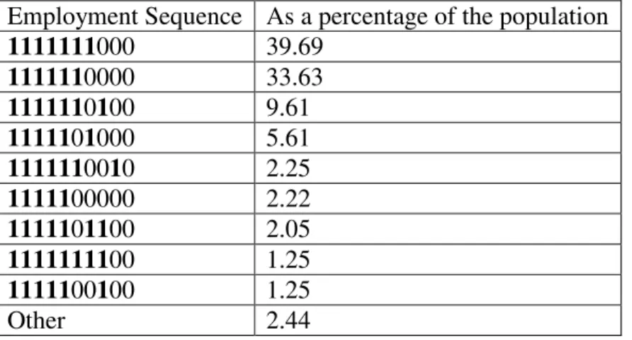
accumulated assets to be substituted for labor income. As Table 2 shows, around 40% retire at period 8, 34%

retire at period 7. 9.61% of them are temporarily unemployed at period 7, employed the next period, and then

retire at period 9. The agents are all identical except that they may realize different wage and return shocks

along their lives, and hence retire at different ages. In the finance literature studying household portfolio

choices, it is always assumed that retirement age is fixed. As we can see in this model (and in the real data), it is

not true. As will be made clear shortly, portfolio allocation decisions are sensitive to plans about retirement. If

the agents' retirement patterns show such variability then a significant amount of variation in the household

portfolios in data could be attributed to different retirement patterns. Hence assuming retirement age to be given

Table 2: Timing of Retirement without Social Security

Employment Sequence As a percentage of the population

1111111

000

39.69

111111

0000

33.63

111111

0

1

00

9.61

11111

0

1

000

5.61

111111

00

1

0

2.25

11111

00000

2.22

11111

0

11

00

2.05

11111111

00

1.25

11111

00

1

00

1.25

Other

2.44

In Figure 1, we see that employment rate is 100% in the first 3 periods, and then it falls gradually to

88% in period 6. Then we see a sharp decline: 50.3% in period 7, 14.6% in period 8, 3.6% in period 9, and 0.1%

4.1.2. Consumption and Assets

Consumption grows with age since the average rate of return on assets (between 1.03 and 1.04,

depending on the portfolio composition) is higher than the rate of time preference (1.02). As a typical life-cycle

model would suggest, the agents accumulate wealth while they are working and decumulate wealth during

4.1.3. Portfolio Allocation

As we will see more clearly in the next section where solution results are presented, portfolio

allocation depends on current cash-on-hand and expected future labor income. If cash-on-hand is very low, then

the agents may prefer not to save, and we have no portfolio decision. If the agent decides to save, then there are

a couple of ways the magnitude of cash-on-hand affects portfolio choice. As explained in Bodie, Merton,

Samuelson (1991), total wealth can be thought of as the sum of human wealth and financial wealth. Human

wealth is the expected total future labor income and financial wealth is the financial assets held. The relative

magnitudes and risks of these two portions of wealth determine current portfolio choice.8

Figure 3 shows the evolution of the average percentage share of risky assets in total financial wealth.

Portfolios are composed of 100% risky asset in the first 3 periods. Starting with the 4th period, we see a

continuous decline until death. This is consistent with the well-known advice given by portfolio managers to

individual investors: Hold a higher percentage of risky assets before retirement, and monotonically decrease the

percentage of risky assets after retirement. The rationale behind that advice is the following: If the expected

future labor income is relatively less risky compared to risky assets held, or if the correlation between future

labor income shocks and return shocks is not significantly positive, then in the earlier stages of life total

expected lifetime wealth has a big less risky component. As the agent approaches the end of the life cycle,

expected labor income, that is, his less risky component of total expected financial wealth, shrinks. Hence the

agents should hold riskier portfolios early in the life cycle and less risky portfolios towards the end of the life

cycle. In the earlier periods of the life-cycle the agents can mitigate the effect of any big adverse return shock

by dissipating its effect to longer future time periods (i.e. by working longer). On the other hand, in the later

stages of life, there are not many periods left.

8

4.1.4. Behavior of Groups of Various Retirement Ages:

I have picked the most populous groups in Table 2 and graphed their consumption, saving, income,

and portfolio allocation paths. These groups are named as follows:

Ret8: The group that consists of simulated agents who work for the first 7 periods, then retire at period

8 and never return to work. This group constitutes around 40% of the population.

Ret7: The group that consists of simulated agents who work for the first 6 periods, then retire at period

Ret7Back8: The group that consists of simulated agents who work for the first 6 periods, then

temporarily retire at period 7, go back to work at period 8, and finally retire at period 9. This group constitutes

around 10% of the population.

In the Figures 4, 5, 6, 7 and 8 below, I depict consumption, assets, income, return shocks, and portfolio

allocation in order to demonstrate how identical agents exhibit different behaviors depending on the shocks

(particularly on return shocks since I have kept the standard deviation of wages very small).

In Figure 4, we see that consumption drops in the period where Ret7 agents retire. This is not because

of a strong adverse shock (See Figure 7). These agents are lucky in the sense that they received big positive

return shocks throughout the first 6 periods, and they were able to save more than the other groups (see Figure

5). Having a lot of savings, realizing an above average return shock in period 7, and the desire not to work

contributes to their decision that they would sacrifice some current consumption in order not to work thereafter.

Almost the opposite scenario applies to Ret8 and Ret7Back8 so that they cannot afford to retire, and they have

to work one more period. Once they decide to work, they have around 20 thousand dollars more, and hence we

see a big increase in consumption. The difference between Ret8 and Ret7Back8 is that the latter group has a

little more assets and they temporarily retire at period 7 only to receive a big adverse return shock in period 8

and go back to employment.

In Figure 8 we see that the Ret7Back8 group has a higher share of risky assets in their portfolio at

period 6, and especially at period 7. Even though Ret7Back8 group has almost same amount of cash-on-hand as

the Ret7 group, they decide to hold more risky financial wealth in period 7 compared to the Ret7 group. Why?

That is because they are more likely to work in period 8 than the Ret7 group. They do not have enough assets

saved to withstand a big adverse return shock in period 8. But it is worth putting a little bit more money on the

risky asset with the hope that a good return will allow them to retire sooner (if they get a good return they would

Figure 5 Average Wealth by Age by Groups of Various Retirement Ages

0 10 20 30 40 50

1 2 3 4 5 6 7 8 9 10

Age A v er a g e A ss et s (i n $ 1 ,0 0 0 ) A-Ret8 A-Ret7 A-Ret7Back8 Figure 6 Average Incomes by Age by Groups of Various Retirement Ages

19.70 19.80 19.90 20.00 20.10 20.20 20.30 20.40

1 2 3 4 5 6

Figure 7

Average Returns on Risky Asset Holdings by Age by Groups of Various Retirement Ages

-4 -2 0 2 4 6 8 10 12

1 2 3 4 5 6 7 8 9 10

Age

A

v

er

a

g

e

%

R

et

u

rn

Return-Ret8 Return-Ret7 Return-Ret7Back8 Return for All

Figure 8

Average Portfolio Allocation by Age by Groups of Various Retirement Ages

0 20 40 60 80 100

1 2 3 4 5 6 7 8 9

Age

%

W

ea

lt

h

H

el

d

i

n

R

is

k

y

A

ss

et

4.2. Simulations with Social Security

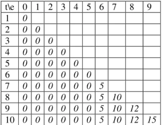
I use the same parameters as simulation 1 other than the social insurance parameters. I used the

following benefit schedule:9

t\e 0 1 2 3 4 5 6 7 8 9 1 0

2 0 0

3 0 0 0

4 0 0 0 0

5 0 0 0 0 0

6 0 0 0 0 0 0

7 0 0 0 0 0 0 5

8 0 0 0 0 0 0 5 10

9 0 0 0 0 0 0 5 10 12

10 0 0 0 0 0 0 5 10 12 15

Table 3: Timing of Retirement with Social Security

Employment Sequence Percent

1111111000

9.54

1111110000

90.10

1111110100

0.36

Table 3 shows that employment patterns are more regular with Social Security because of the

incentives to retire at certain times provided by the system. Around 90% of the agents retire at period 7, when

they are eligible for a relatively small early retirement benefit.

Figure 9 shows average consumption and saving paths. We see that this social insurance program

depresses savings, and average consumption in the Social Security case is higher by about $1,000 at every point

in time compared to the one with no Social Security.

9

Figure 10 shows that until period 8, optimal portfolios are more risky without the social insurance

system. One factor contributing to this should be that for 90% of the simulated agents future income in the

simulation with Social Security is 5 for every period after 6, and that is small relative to assets held. Hence the

inherent risk in total wealth is bigger in simulations with Social Security, and thus less risky portfolios are

optimal. In the last 2 periods optimal portfolios in the SS case are a little more risky than the ones in no SS case.

That could be because there is almost no chance to be working in the last 2 periods in no SS case. Hence there is

less non-risky human wealth remained in no SS case compared to SS case. Thus agents may be holding less

risky portfolios in no SS case compared to SS case.

Figure 9

Average Consumption and Assets by Age with and without Social Security

0 5 10 15 20 25 30 35 40

1 2 3 4 5 6 7 8 9 10

Age

A

v

er

a

g

e

in

$

1

,0

0

0

's

Figure 10

Average Portfolio Allocation by Age with and without Social Security

0.0 20.0 40.0 60.0 80.0 100.0 120.0

1 2 3 4 5 6 7 8 9

Age

%

W

ea

lt

h

h

el

d

i

n

R

is

k

y

A

ss

et

(

A

v

er

a

g

e)

Portfolio Portfolio with SS

5. Analyzing the Solution in More Detail

Analyzing the solution of the model we can get a more detailed idea about how the model works. In

the literature, generally simulations are presented but examining the solution patterns gives the most detailed

information on the model dynamics.

The following 3 graphs depict how the solution (optimal consumption and portfolio allocation)

changes with respect to cash-on-hand in the last three periods (period 9, 8, and 7 respectively). For period 9, I

Figure 11

Figure 13

When we examine the graphs we make the following observations:

1) Consumption: There are abrupt consumption drops. The number of consumption drops is equal to

the number of periods left.

2) Portfolio Allocation: There is a general downward trend, and there are some spikes in between. The

number of spikes is same as the number of periods left.

I will show that the reason behind the jumps in the portfolio allocation and consumption is the

"sudden"10 changes in expected future income.11

The following two factors have important roles in the sudden big drops in consumption: 1) The strong

desire not to work: Individuals either work or don’t work. Once they decide to work, they face a big negative

utility loss due to the additive marginal disutility of work component of the utility function. 2) The utility

function, which is very steep at low levels of consumption and flat at higher levels of consumption. So,

although the benefit of working (through increased income) can be very low at relatively higher levels of

consumption, the utility cost of working may be very high, which does not depend on consumption level.

Hence, the agents are willing to forego a big chunk of consumption today in order to afford not to work next

period.

To illustrate that reasoning let us consider Figure 12 and trace optimal consumption relative to

cash-on-hand. For small values of cash-on-hand (up until about $19,500) the agent does not save at all. He consumes

everything. That is because the cash-on-hand he has is too small to maintain minimal consumption levels in

period 9 and period 10. Since the utility function is very steep at those relatively small levels of consumption,

10

The word "sudden" is used in the sense that for a small change in cash-on-hand, we may see abrupt changes in optimal consumption and portfolio allocation.

11_{We will see that the sudden changes in portfolio allocation and also in consumption happen at the points where the}

he realizes that he will have to work next period: The penalty for not working next period (that is, getting very

low levels of utility from consumption in this and the future period) is even worse than the stiff utility penalty

for working next period. Since he knows he will be working next period, there is no need to save now. Enjoy

consumption today, and tomorrow's consumption will be completely financed by tomorrow's labor income.

If we keep increasing cash-on-hand, at some point the agent will have enough cash-on-hand to afford not to

work next period. At that point savings has to jump from 0 to a not-so-small positive number since, due to the

shape of the utility function, miniscule levels of next period consumption cannot be optimal.

To help understand the patterns in portfolio allocation solutions consider the following two possible

cases:

Case 1: Corner Solution. Financial wealth can be a very small fraction of total wealth (especially in

early periods). Then the total wealth is dominated by human wealth. If future labor earnings are not very risky,

then the overall riskiness of total wealth may be too low and the agents may find it optimal to invest all their

financial wealth in the risky asset.

Case 2: If the share of financial wealth in total wealth gets bigger, and we keep everything else equal,

then we would expect a smaller percentage of risky assets held compared to the previous case.

If we examine the solutions carefully, we can see these two effects in play both within a period and

across periods.

Within a given period, changing cash-on-hand changes the share of financial wealth in total wealth.

For the moment let's focus on each smooth part of the portfolio allocation that are between the spikes

separately. All of them are smoothly declining. Explanation: If the expected future employment sequence is

roughly constant, then increasing cash-on-hand (hence increasing the more risky component of wealth, financial

Now notice that the lowest point of each smooth part (in between the spikes) is lower than its

counterparts, which are to the left. Explanation: The magnitude of cash-on-hand determines the probabilities of

expected future employment sequences. If we keep increasing cash-on-hand, at some point, the forward looking

agent will realize that he may have enough cash-on-hand to retire one period early. At this point we may

observe a fast change of probabilities of future employment sequences. Portfolio allocation responds to this

change of future employment probabilities: If it is likely now that the agent is going to work for one less period,

then he has to hold a less risky portfolio since the share of risky wealth in total wealth has grown.

Across periods: The same level of cash-on-hand implies different portfolio allocations in different

periods simply because the composition of the total changes over time.

Now it is time for the spikes: Above, I have described some of the main channels through which

portfolio allocation is affected. The results that we see are far richer than that. The interaction between the

magnitude of cash-on-hand and probabilities of future employment creates possibilities for optimal portfolio

allocation to vary a lot. For example in addition to the cases described above, think of the "gray" areas where

the agent has such an amount of cash-on-hand such that he is neither very likely to work nor very unlikely to

work in a future period. In those cases the agent may gamble now for a chance to avoid working next period. He

may prefer to hold a riskier financial portfolio hoping that, next period, he may get returns high enough that he

will not have to work. If he is lucky he will get a huge utility boost. If not, he may not "suffer" too much in the

sense that it was already probable that he would work next period, and now he will have more cash-on-hand

(because of the labor income) to be spent on consumption.

In the light of the explanations above, now let's reexamine the portfolio allocation decisions by looking

at the above 3 figures: Portfolio allocation (x) versus cash-on-hand in period 9, period 8, and then 7:

In period 9, x is constant just the way it is in the simplest form of dynamic portfolio choice model of

the risky asset. Our model is more general than his, but period 9 is a special case since the future horizon is only

1 period and the agents are certain that they are not going to work if they decide to save.

Note that for all periods the number of consumption drops is same as the number of periods left. That

is not a coincidence. At those points where consumption drops abruptly, probabilities of future employment

change abruptly too. Once the agent thinks that saving more aggressively allows him to retire one period earlier,

he is willing to take a big consumption drop. This is very clear in period 9 since only 1 period is ahead. But, the

earlier periods we analyze are more complicated since there is now interaction between possible future

employment sequences.

In periods 8 and 7 we see two things: The optimal share of risky assets is a monotonic decreasing

function of cash-on-hand, and the optimal share suddenly jumps to a higher value two times in period 8 and 3

times in period 7. Again, this is because of the way the probabilities of future employment sequences change.

Consider period 8: For small values of cash-on-hand agents do not save. For a little higher value agents save

and plan to work for the next 2 periods. If they have a little more cash-on-hand they may plan to work for 1

period less, and finally if they have a huge amount of savings they figure they will never work. These are where

we see the jumps in x.

To see whether the jump in consumption is the result of using a "not fine enough" grid, I solve the

model with 10 times more grid points for cash-on-hand, that is I use 2,000 grid points rather than 200. We still

see the jumps in consumption and portfolio choice.

To better understand the reason behind the jump, I calculate and report the probability of next period

employment at period 9. I report this for period 9 because at this period there are only two possible future

employment patterns: work and not work. If I were to use previous periods, then the number of possible future

employment patterns increase exponentially. As I have explained previously, the reason of the jump is the

"sudden" big changes in the probability of next period employment. I report the relationship between the

it is calculated after the agents optimally choose consumption and portfolio allocation given cash-on-hand. We

will see below that as cash-on-hand increases, at some point the probability jumps down from 100% to 0%. To

help visualize how that probability jumps, I also present the relationship between the probability of next period

employment and consumption-portfolio allocation pairs at a given cash-on-hand. There we will see, in some

regions, how extremely sensitive that probability is to changes in either consumption or portfolio choice.

The way I calculate the probabilities is simple: Due to the nature of dynamic programming, we already

had to take into account every possible future event in calculating optimal decisions. I just modified the

program to keep track of whether the agent works or not in every case. Then I simply calculate the ratio of the

number of cases in which the agent works to the number of total cases. The number of total cases is 10,000

since it is the number of draws I use in Monte Carlo integrations.