Aminian_unc_0153D_16671.pdf

THE ROLE OF CROSS SECTIONAL GEOMETRY IN THE PASSIVE

TRACER PROBLEM

Manuchehr Aminian

A dissertation submitted to the faculty at the University of North Carolina at Chapel Hill in partial

fulfillment of the requirements for the degree of Doctor of Philosophy in the Department of

Mathematics in the College of Arts and Sciences.

Chapel Hill

2016

Approved by:

Roberto Camassa

Richard McLaughlin

David Adalsteinsson

Laura Miller

ABSTRACT

Manuchehr Aminian: The role of cross sectional geometry in the passive

tracer problem

(Under the direction of Roberto Camassa and Richard McLaughlin)

This dissertation is concerned with how the longitudinal moments (mean, variance, skewness)

of a tracer distribution undergoing an advective-diffusive process in Poiseiulle flow depend in a

nontrivial way upon the cross section of the pipe.

ACKNOWLEDGEMENTS

I would like to recognize the significant role my friends played in motivating me to get to work,

and the patience of my advisors when I didn’t work.

On a more serious note, the significant progress we’ve made in the work related to this dissertation

would not have happened if not for the support of the others in our research group: Francesca

Bernardi, Dan Harris, and my advisors, Rich McLaughlin and Roberto Camassa.

TABLE OF CONTENTS

LIST OF FIGURES . . . .

xii

LIST OF TABLES . . . .

xv

CHAPTER 1: INTRODUCTION . . . .

1

CHAPTER 2: NOTATION AND SETUP . . . .

3

2.1

Derivation of the model equations . . . .

3

2.2

Flow solution in the infinite channel

. . . .

4

2.3

Flow solution in the circular pipe . . . .

5

2.4

Flow solution in the rectangular pipe . . . .

5

2.5

Flow in elliptical pipes . . . .

7

2.6

Advection diffusion equation . . . .

8

CHAPTER 3: ASYMPTOTICS OF THE ARIS EQUATIONS . . . .

9

3.1

The Aris equations. . . .

9

3.2

Short time asymptotics of the Aris equations. . . .

11

3.2.1

Exact moments without diffusion. . . .

11

3.2.2

Pointwise statistics of a passive tracer with advection alone. . . .

12

3.2.3

Averaged statistics of a passive tracer with pure advection. . . .

13

3.2.4

Short time asymptotics with diffusion. . . .

16

3.2.5

Comparison of short time asymptotics and simulation. . . .

20

3.3

Long time asymptotics of the Aris equations.

. . . .

22

3.3.1

Long time asymptotics of with a polynomial time driver. . . .

24

3.3.2

Long time behavior of the Aris equations. . . .

25

3.3.4

Exact calculation of long time asymptotics in any ellipse.

. . . .

28

3.3.5

Calculation of long time coefficients in the rectangular duct. . . .

31

CHAPTER 4: POISSON SUMMATION OF CHANNEL FORMULAE . . . .

35

4.1

Motivation . . . .

35

4.2

Derivation of the seed identity . . . .

36

4.3

Poisson summation of

T1

. . . .

40

4.3.1

The

p

= 2

case . . . .

40

4.3.2

The

p

= 4

case . . . .

42

4.3.3

Poisson summation for the first moment in the channel . . . .

43

4.3.4

Verifying conserved quantities . . . .

45

4.3.5

Summary . . . .

47

4.4

Poisson summation of the second moment in the channel . . . .

47

4.4.1

The

p

= 6

case . . . .

48

4.4.2

The

p

= 5

case . . . .

49

4.4.3

The

p

= 8

case . . . .

50

4.4.4

The

p

= 7

case . . . .

51

4.4.5

Expression for

T

. . . .

51

4.5

Third moment in the channel and comparison for centered statistics

. . . .

52

4.6

Summary of identities . . . .

57

CHAPTER 5: MONTE CARLO SIMULATION . . . .

60

5.1

Brownian motions and their connection to advection-diffusion problems

. . . .

60

5.2

Implementation of the Monte Carlo method . . . .

63

5.2.1

Specifying the initial conditions . . . .

63

5.2.2

Calculation of the flow . . . .

65

5.2.3

Implementation of diffusion and enforcing boundary conditions . . . .

65

5.2.4

Calculation of statistics . . . .

69

5.3

Validation and convergence of numerics

. . . .

71

5.3.1

Validation in the infinite channel . . . .

71

5.3.3

Validation through long time asymptotics . . . .

75

5.4

Results in the rectangular and elliptical domains

. . . .

77

CHAPTER 6: NUMERICS AND ASYMPTOTICS IN OTHER DOMAINS . . .

79

6.1

Introduction . . . .

79

6.2

Racetrack cross sections . . . .

79

6.2.1

Derivation of the flow

. . . .

79

6.2.2

Monte Carlo simulation for the racetrack . . . .

82

6.3

Triangular cross section

. . . .

84

6.3.1

Calculation of the flow . . . .

84

6.3.2

Calculation of asymptotics . . . .

85

6.3.3

Modification of Monte Carlo code . . . .

85

6.3.4

Asymptotics in the regular polygons . . . .

87

APPENDIX A: SOLUTIONS TO ASYMPTOTICS IN THE ELLIPSE. . . .

90

A.1 Explicit solution of the

g

(ξ, η)

problem in the ellipse . . . .

90

A.2 Solution of the

g

(ξ, η)

problem in the ellipse

. . . .

91

APPENDIX B: SOURCE CODE FOR MONTE CARLO SIMULATIONS. . . . .

95

B.1 Necessary packages and compilers . . . .

95

B.2 ./ . . . .

96

B.2.1

./makefile

. . . .

96

B.2.2

./parameters_mc.txt

. . . .

97

B.2.3

./batch_submit.py

. . . .

98

B.3

./monte/

. . . 100

B.3.1

./monte/channel_mc.f90

. . . 100

B.3.2

./monte/duct_mc.f90

. . . 108

B.3.3

./monte/ellipse_mc.f90

. . . 118

B.3.4

./monte/racetrack_mc.f90

. . . 128

B.3.5

./monte/triangle_mc.f90

. . . 137

B.4.1

./utils/buffer_op_channel.f90

. . . 147

B.4.2

./utils/buffer_op_duct.f90

. . . 148

B.4.3

./utils/channel_mc_messages.f90

. . . 148

B.4.4

./utils/check_ic_channel.f90

. . . 149

B.4.5

./utils/check_ic_duct.f90

. . . 150

B.4.6

./utils/correct_tstep_info.f90

. . . 150

B.4.7

./utils/duct_mc_messages.f90

. . . 151

B.4.8

./utils/findcond.f90

. . . 152

B.4.9

./utils/generate_internal_timestepping.f90

. . . 153

B.4.10

./utils/generate_target_times.f90

. . . 153

B.4.11

./utils/get_pts_in_ellipse.f90

. . . 155

B.4.12

./utils/get_pts_in_triangle.f90

. . . 156

B.4.13

./utils/get_racetrack_area.f90

. . . 158

B.4.14

./utils/hdf_add_1d_darray_to_file.f90

. . . 159

B.4.15

./utils/hdf_add_2d_darray_to_file.f90

. . . 160

B.4.16

./utils/hdf_add_3d_darray_to_file.f90

. . . 162

B.4.17

./utils/hdf_create_file.f90

. . . 163

B.4.18

./utils/hdf_read_1d_darray.f90

. . . 164

B.4.19

./utils/hdf_write_to_open_2d_darray.f90

. . . 165

B.4.20

./utils/interp_meshes.f90

. . . 167

B.4.21

./utils/linear_interp_2d.f90

. . . 168

B.4.22

./utils/make_filename_direct.f90

. . . 171

B.4.23

./utils/make_histogram.f90

. . . 171

B.4.24

./utils/make_histogram2d.f90

. . . 173

B.4.25

./utils/my_normal_rng.f90

. . . 174

B.4.26

./utils/print_parameters.f90

. . . 176

B.4.27

./utils/progress_meter.f90

. . . 178

B.4.28

./utils/read_inputs_direct.f90

. . . 179

B.4.29

./utils/read_inputs_mc.f90

. . . 179

B.4.31

./utils/save_the_rest_duct.f90

. . . 184

B.4.32

./utils/set_initial_conds_channel_mc.f90

. . . 186

B.4.33

./utils/set_initial_conds_duct_mc.f90

. . . 188

B.4.34

./utils/set_initial_conds_ellipse_mc.f90

. . . 190

B.4.35

./utils/set_initial_conds_racetrack_mc.f90

. . . 192

B.4.36

./utils/set_initial_conds_triangle_mc.f90

. . . 194

B.4.37

./utils/solve_quadratic_eqn.f90

. . . 197

B.4.38

./utils/sortpairs.f90

. . . 197

B.4.39

./utils/uniform_bins_idx.f90

. . . 199

B.4.40

./utils/vector_ops.f90

. . . 199

B.4.41

./utils/walkers_in_bin_1d.f90

. . . 201

B.4.42

./utils/walkers_in_bin_2d.f90

. . . 202

B.4.43

./utils/write_outputs_direct.f90

. . . 203

B.4.44

./utils/write_outputs_mc.f90

. . . 203

B.4.45

./utils/zeroout.f90

. . . 204

B.5

./computation/

. . . 205

B.5.1

./computation/Alpha_eval.f90

. . . 205

B.5.2

./computation/Beta_tilde.f90

. . . 205

B.5.3

./computation/accumulate_moments_1d.f90

. . . 206

B.5.4

./computation/accumulate_moments_2d.f90

. . . 208

B.5.5

./computation/apply_advdiff1_chan.f90

. . . 211

B.5.6

./computation/apply_advdiff1_duct.f90

. . . 212

B.5.7

./computation/apply_advdiff1_ellipse.f90

. . . 213

B.5.8

./computation/apply_advdiff1_racetrack.f90

. . . 215

B.5.9

./computation/apply_advdiff1_triangle.f90

. . . 216

B.5.10

./computation/apply_advdiff2_chan.f90

. . . 218

B.5.11

./computation/asymp_st_channel_moments.f90

. . . 219

B.5.12

./computation/impose_reflective_BC_ellipse.f90

. . . 220

B.5.13

./computation/impose_reflective_BC_polygon.f90

. . . 223

B.5.15

./computation/impose_reflective_BC_rect.f90

. . . 232

B.5.16

./computation/matvec.f90

. . . 233

B.5.17

./computation/moments.f90

. . . 234

B.5.18

./computation/precalculate_Alpha.f90

. . . 235

B.5.19

./computation/precompute_uvals.f90

. . . 236

B.5.20

./computation/precompute_uvals_ss.f90

. . . 237

B.5.21

./computation/racetrack_bdist.f90

. . . 238

B.5.22

./computation/u_channel.f90

. . . 239

B.5.23

./computation/u_duct.f90

. . . 239

B.5.24

./computation/u_duct_precomp.f90

. . . 240

B.5.25

./computation/u_duct_ss.f90

. . . 240

B.5.26

./computation/u_dummy.f90

. . . 242

B.5.27

./computation/u_ellipse.f90

. . . 242

B.5.28

./computation/u_racetrack.f90

. . . 242

B.5.29

./computation/u_triangle.f90

. . . 243

B.6

./modules/

. . . 244

B.6.1

./modules/mod_ductflow.f90

. . . 244

B.6.2

./modules/mod_duration_estimator.f90

. . . 244

B.6.3

./modules/mod_readbuff.f90

. . . 246

B.6.4

./modules/mod_time.f90

. . . 246

B.6.5

./modules/mod_triangle_bdry.f90

. . . 246

B.6.6

./modules/mtfort90.f90

. . . 247

LIST OF FIGURES

3.1

Flow profiles for the rectangular (solid colors) and elliptical duct (white lines) of

aspect ratio

λ

= 0.4, scaled to match the peak velocity.

. . . .

21

3.2

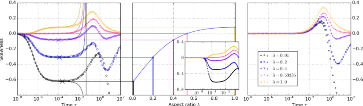
Evolution of skewness for the rectangles (left panel) and ellipses (right panel) of varying

aspect ratio. Geometric skewness is plotted (center panel) as a function of aspect

ratio, with aspect ratios corresponding to the simulations indicated. Simulations done

using a finite width initial condition

σ

≈

0.115

in the rectangles (inset) are done with

the same aspect ratios. In all cases, Pe

= 10

.

. . . .

22

4.1

Comparison of the original summation to the expression recast via Poisson summation

in (4.12). Top row: both original and Poisson versions truncated to

100

terms for

times

t

= 10

, ...,

10

on the

y-interval

[−1,

1]. Bottom row: demonstration of the

terms needed for convergence scaling like

N

∼

√

t

in the boundary layer. Here,

t

= 10

, and

Nmax

is varied from

10

to

10

.

. . . .

38

4.2

Behavior of (4.14) when keeping a small number of images at small to intermediate

time. The effect of the extra images is not seen until order one time. . . .

39

4.3

Evaluation of the left and right-hand sides of (4.23) and (4.24) with

N

= 10

for

the original summation. The effect of neglecting the

Er(·)

terms is seen by

t

= 10

.

42

4.4

Evaluation of the left and right-hand sides of (4.30) with

N

= 10

for the original

summation (black), no extra images as in (4.31) (green), and two extra images kept

(red).

. . . .

43

4.5

Evaluation of the left and right-hand sides of (4.47) with

N

= 10

for the original

summation (black), only the

±1

images (green), and the

±1,

±3

images (red). As

with previous cases, only two images are needed until order one time.

. . . .

49

4.6

Evaluation of (4.64) with

Nmax

= 10

for the original summation (black), and the

Poisson summation equivalents keeping only the

±1

images (green circles), and the

first forty images centered around

[−1,

1]

(red stars). Green circles not shown in the

final panel.

. . . .

52

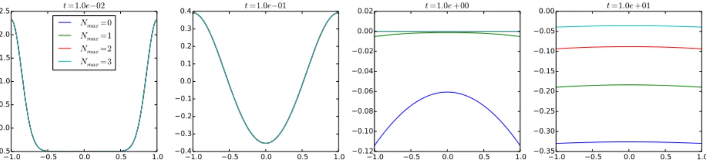
4.7

Evaluation of the channel variance (top rows) and skewness (bottom rows) with

5.1

Illustration of a reflecting boundary condition in one dimension (left panel) and two

dimensions in the case of the duct near the corner (right panel). The exterior of the

domain is indicated with hatches. The channel reflections have a simple formula for

preserving the total distance traveled. The rectangle requires dealing with corner

cases, where one needs to find the minimum of intersection times

{s

, s

}

(green

circles) and multiple reflections. The right panel illustrates that the domain can be

implicitly defined where a function

u(y, z)

>

0.

. . . .

68

5.2

Left panel: Time evolution of the numerical (shades of red) and exact skewness (black)

of the averaged distribution in the channel for Péclet values Pe

= 10

,

10

,

10

and

number of particles

N

= 10

. Right panels, clockwise from top left: snapshots of

the numerical and exact pointwise mean, variance, and skewness for Pe

= 10

, at

t

= 10

. Dashed black lines indicate the zero line of the mean, variance, and skewness.

72

5.3

Analyzing convergence of numerics with increasing

N

. Left panel: absolute error

in the averaged skewness

|Sk(t)

−

Skexact(t)|

in the channel for Péclet values Pe

=

10

,

10

,

10

and numbers of particles

N

= 10

, ...,

10

. Right panel: the corresponding

average error of

|Sk(ti)

−

Skexact(ti)|

is plotted versus the number of particles, with a

power law fit. The expected scaling of error as

1/

√

N

is generally observed. . . .

72

5.4

Analyzing convergence of numerics with

N

= 10

and Pe

= 10

fixed, with decreasing

∆tmax

. Ten simulations are run for each

∆tmax

, and the range of errors is shown. The

error behaves nonrandomly for

∆t

≥

10

, growing at an approximately linear

rate in time until the hard cap is hit. The error then decays as both the numerics

and exact solution begin decaying to zero around

t

≈

10

.

. . . .

73

5.5

Time evolution of the numerical (shades of red) and exact (black) skewness in the

circular pipe for Péclet values Pe

= 10

,

10

,

10

and number of particles

N

= 10

.

General agreement is seen across a range of Péclet values, except at short time, where

the exact formulae have numerical cancellation issues, and a deviation near

τ

≈

10

_.

₇₄

5.6

Analyzing convergence of numerics in the circular pipe with increasing

N

. Left panel:

absolute error in the averaged skewness

|Sk(t)

−

Sk

(t)|

in the pipe for Péclet

values Pe

= 10

,

10

,

10

and numbers of particles

N

= 10

, ...,

10

. Right panel: the

corresponding average error of

|Sk(t

)

−

Sk

(t

)|

is plotted versus the number of

particles, with a power law fit. The expected scaling of error as

1/

√

N

is generally

observed.

. . . .

75

5.7

Behavior of the skewness

Sk

in the numerics for various geometries. Top row: skewness

evolution for ellipses (left) and rectanges (right) of varying aspect ratio with Pe

= 10

.

Bottom row: log-log plot of

|Sk|

versus time for the ellipses (left) and rectangles

(right).

. . . .

76

5.8

Snapshots of the pointwise skewness in the ellipses and rectangles. Aspect ratios

6.1

Illustration of the racetrack for the choices of parameter pairs shown. Note that for

s < λ

it is common for the domain to be come non-convex, as can be seen with

(λ, s) = (0.5,

0.35). The hatched regions indicate the exterior of the domain, and red

and blue indicate regions where

u >

0

and

u <

0

respectively. . . .

81

6.2

Averaged skewness over a range of parameter pairs

(λ, s)

which satisfy a convexity

criterion at

(y, z) = (1,

0), plotted at nondimensional times (from left to right)

t

≈

0.015,

0.97, and

6.28. Positive (negative) skewness is red (blue), with white being

zero. An approximate zero skewness contour is overlaid in black. Long time behavior

is seen to be nearly independent of the shape parameter.

. . . .

84

6.3

Demonstration of the reflection algorithm for some convex polygons. An extremely

long trajectory is taken, then the reflection algorithm is applied iteratively until the

final position

(y

, z

)

is in the domain. The number of reflections is illustrated in the

changing color. Left: equilateral triangle with eight reflections. Center: Reflection

in a rectangle

λ

= 1/2

whose initial outward trajectory has a rational slope. Right:

demonstration in a non-regular octagon of the same aspect ratio. . . .

87

6.4

Results in the triangular geometry. Left: schematic of the flow profile, with

y

= 0

and

z

= 0

lines. Center: skewness in fifty simulations (black) and short time (red)

and long time (blue) asymptotics, with Pe

= 10

. Right: the same simulations and

long time asymptotics with log-scaled axes.

. . . .

88

6.5

Visualization of the numerically computed flow profile in the regular

n-gons for

LIST OF TABLES

4.1

Absolute error of the “mass" for the truncated Poisson summations (4.34), and the

truncation when dropping

Er(·)

terms, (4.35) evaluated at different times. Dropping

the

Er

terms is seen to violate the total mass condition in a quadratic fashion.

. . .

46

4.2

Polynomials

q

,

p

= 0,

1, ...,

12

necessary for Poisson summation of the solutions for

the first three moments in the channel. . . .

59

6.1

Geometric skewness and the long time coefficient

3hug2

i/(2hug1

i)

_calculated

nu-merically for the regular

n-gons. The coefficients monotonically approach the circle

(n

=

∞) value, disproving the conjecture that there may be an even/odd parity in

CHAPTER 1

Introduction

The study of passive tracers under the influence of laminar fluid flow was first brought to the

limelight by G.I. Taylor, whose paper in 1953 [1] demonstrated with experiment and theory how

the effective diffusivity, as measured by the rate of growth of mean squared displacement of tracer

relative to its mean, is much more rapid than would be expected due to draw molecular diffusion

when put under the influence of laminar pipe flow. The fundamental result is that the enhancement

of diffusivity is proportional to

R

U

/κ, where

R

is the pipe radius,

U

is the characteristic speed of

the fluid flow, and

κ

the molecular diffusivity.

Dynamically, the tracer is asymptotically Gaussian at both very short times and very long times,

as measured relative to the diffusive timescale

t

∝

R

/κ. However, he observed that at intermediate

times the distribution of tracer was highly non-Gaussian.

Since then, many others have studied this result. One main tool came from Aris [2], who showed

that the tracer

T

, whose evolution is modeled by the advection diffusion equation, can more readily be

studied by the evolution of its longitudinal (flow-wise) moments, which themselves obey a hierarchy

of driven diffusion equations. He, along with many others [3, 4, 5], derived results, both exact and

asymptotic in time, for the case of the circular pipe and infinite parallel plate (“channel") flow. In

another vein, the long time effective diffusivity was studied for a pipe of general rectangular or

elliptical cross section [2, 6].

More recently, the problem has been revisited with the tools of homogenization theory, which

have been used to derive more detailed predictions in the channel and circular pipe cases with

arbitrary point source release [7, 8], and in the case of pulsatile (time-oscillatory) flows [9].

of the influence of the cross section on the distribution of the tracer. Several papers have addressed

this, but are usually only interested in effective diffusivity [10, 11, 12, 13]. Attention has also been

paid in the arena of blood flow and drug delivery [14], despite the necessary assumptions of laminar,

Newtonian fluid flow being dubious for blood.

However, very little attention has been paid since the early papers of Aris [2], Chatwin [3], and

Barton [5] towards the asymmetry induced by the fluid flow. In the two simplest cases of circular

pipe and infinite channel, it turns out that the tracer exhibits opposite signs of the skewness (the

centered, normalized third moment) when examining the cross-sectional average.

In other words, despite the flow solutions being mathematically similar, they produce opposite

asymmetries in the distribution! This was in fact the original motivation for this dissertation work.

Following from this original question, we were motivated to examine how the skewness behaves

for different classes of cross sections to see if we could connect the purely positive skewness of the

circular cross section to the purely negative skewness in the channel. To do this, we first examined

the family of rectangular and elliptical cross sections, establishing both short time and long time

asymptotics of the Aris moment equations. This revealed that the short time skewness is in fact

zero for all ellipses, and sign-indefinite for the rectangles, with a “golden" aspect ratio (the ratio

of short to long sides) of

λ

≈

0.53335

which has similar statistical behavior to the ellipses. We

followed through with the long time analysis to demonsrate that both the rectangles and ellipses

have sign-indefinite skewness at long time, separated by an aspect ratio

λ

≈

0.49. We wrote a Monte

Carlo method, which shows strong agreement across a wide range of benchmarks, yielding additional

support to our results. Finally, we considered a number of extensions to other cross sections which

permitted analysis and/or simulation, such as the equilateral triangle, the class of regular polygons,

and perturbations of the ellipses, which exhibit a wide range of behaviors.

In broad strokes, the main results of this dissertation work are that the longitudinal skewness of

a passive tracer in a laminar fluid flow has strong dependence on the shape of the cross section of

the pipe. Depending on the application of interest, this permits a degree of control in how the tracer

is delivered to its final destination.

1

CHAPTER 2

Notation and Setup

In this chapter, we derive the partial differential equation for the fluid velocity in a generic

domain and give the solution in a few classes of domains. We also introduce the advection diffusion

equation for the tracer.

Derivation of the model equations

First we derive the partial differential equations for the fluid flow. In general, the Navier-Stokes

equations describes the evolution of the fluid velocity field

u

= (u, v, w)

in space and time:

ρ

∂

u

∂t

+

u

· ∇

u

=

−∇p

+

µ∇

u

,

(2.1)

with density

ρ, pressure field

p, and dynamic viscosity

µ. Nondimensionalizing the variables as

x

=

a

x

,

u

=

U

u

,

t

= (a/U

)t

,

p

= (µU/a)p

, with characteristic length and velocity scales

a

and

U

respectively, and using a constant density

ρ

=

ρ0

results in the nondimensionalized form

Re

∂

u

∂t

+

u

_{· ∇}

_u

=

−∇

p

+

∇

u

∇

·

u

= 0.

(2.2)

The coefficient Re

=

ρ0aU/µ

is the Reynolds number. We assume Re

1

and work with the reduced

equations (dropping primes)

∇

u

=

∇p,

∇ ·

u

= 0.

(2.3)

pipe, that is,

u

=

0

on the boundaries. Explicitly we have

∇

u

=

px,

u|

= 0,

(2.4a)

∇

v

= 0,

v|

= 0,

(2.4b)

∇

_w

_{= 0,}

_w|

∂Ω

= 0,

with

(2.4c)

ux

+

vy

+

wz

= 0.

(2.4d)

It is a fact that Laplace’s equation with zero boundary conditions only has the zero solution, so

v

=

w

= 0. Incompressibility gives us that

u

= 0, so that

u

=

u(y, z). We need only to solve

∂

_u

∂y

+

∂

_u

∂z

=

px,

u|

= 0,

px

constant.

(2.5)

We note that, while the equations are nondimensional here, an almost identical derivation holds for

the dimensional flow, with an extra factor of

1/µ

multiplying the pressure gradient. The justification

for dropping the inertial terms in the Navier-Stokes equations comes down to a Reynolds-number-like

argument, where one would assume inertial effects are negligible compared to the viscous and pressure

effects. Functionally the two forms are essentially the same, and we may use the dimensional or

nondimensional form as appropriate.

Flow solution in the infinite channel

Working in dimensional variables with a cross section of infinite parallel plates (a “channel")

Ω =

{(y, z

) :

−a

≤

y

≤

a},

(2.6)

the boundary conditions for the flow problem

∂

u

∂y

+

∂

u

∂z

=

p

µ

,

u|

= 0

(2.7)

imply there is no

z

dependence, so we have an ordinary differential equation for

u(y):

d

u

dy

=

p

which has the solution

u(y) =

−

a

_px

2µ

1

−

(y/a)

.

(2.9)

We set

U

=

−a

_px/µ

_{and include an extra factor of 2 in nondimensional form (for convenience) to}

get a nondimensional flow

u(y) = 1

−

y

.

(2.10)

Flow solution in the circular pipe

Working in dimensional variables with a circular cross section

Ω =

{(y, z) :

y

+

z

≤

a

},

(2.11)

the flow problem is easiest solved using polar coordinates

(y, z

)

→

(r, θ). Additionally assuming a

radially symmetric solution

u(r)

(justified after the fact by uniqueness of solution to the PDE) the

problem reduces to an ODE for

u(r):

1

r

∂

∂r

r

∂u

∂r

=

p

µ

,

u(a) = 0.

(2.12)

This has a functionally similar solution to the parallel plate case:

u

=

−

a

_p

x

4µ

1

−

(r/a)

=

−

a

_p

x

4µ

1

−

(y/a)

2

₋

_(z/a)

.

(2.13)

Letting

U

=

−a

_px/µ

_{and multiplying by a factor of two gives the nondimensional flow}

u

=

1

2

(1

−

r

2

_{) =}

1

2

(1

−

y

2

₋

_z

_).

_(2.14)

Flow solution in the rectangular pipe

In this case, the dimensional domain is

The flow problem does not reduce as much as in the previous cases:

∂

_u

∂y

+

∂

_u

∂z

=

p

µ

,

u|

=

u|

= 0.

(2.16)

In this case, the solution can be written either as an eigenfunction expansion in the form

u(y, z

) =

∞

X

m,n=1

umn

cos((m

−

1/2)πy/a) cos((n

−

1/2)πz/b)

(2.17)

or in a single series, as a correction of the channel flow. The rough interpretation here is that the

channel flow

u

(y)

is the limit of the rectangular case if we send the far walls to infinity, that is,

b

→ ∞. This form of the solution is

u(y, z) =

uc(y) +

∞

X

k=1

ck

cos((k

−

1/2)πy/a) cosh((k

−

1/2)πz/a).

(2.18)

This second form is more convenient in nearly all cases, so we derive the formulae for the coefficients

ck

.

First, the Poisson equation itself is satisfied, since the PDE is linear,

u

(y)

satisfies the equation, and

the terms in the summation

cos((k

−

1/2)πy/a) cosh((k

−

1/2)πz/a)

are harmonic. The boundary

conditions at

y

=

±a

are satisfied independently by every term in the expression. Requiring

u|

= 0,

0 =

uc(y) +

∞

X

k=1

c

cos((k

−

1/2)πy/a) cosh((k

−

1/2)πb/a).

(2.19)

For convenience define

φ

= cos((k

−

1/2)πy/a. Multiplying both sides by

φ

, integrating over

[−a, a], and using the smoothness of the solution to allow the exchange of integration and summation

leads to the formula for the coefficients:

−

Z

u

(y)φ

dy

=

Z

φ

X

c

cosh((k

−

1/2)πz/a)φ

(2.20a)

−

Z

u

(y)φ

dy

=

∞

X

k=1

c

cosh((k

−

1/2)πb/a)

Z

φ

φ

dy

(2.20b)

−

R

−a

u

(y)φ

dy

R

φ

dy

=

cj

cosh((j

−

1/2)πb/a)

(2.20c)

⇒

cj

=

−a

_px

µ

2(−1)

The form of the coefficient gives rapidly converging series, especially for small aspect ratios

λ

=

a/b

1

even without the factor of

(j

−

1/2)

.

To analyze the behavior for large aspect ratios, let

ζ

=

z/b,

α

= (j

−

1/2)πb/a. Then the aspect

ratio dependence in the sum is written as

cosh(αζ)

cosh(α)

,

−1

≤

ζ

≤

1,

(2.21)

and for

α

→ ∞

(i.e., sending the inverse aspect ratio

b/a

→ ∞) this converges pointwise to zero for

ζ

∈

(−1,

1)

and to one for

ζ

=

±1. (This can be shown with standard analysis techniques.)

Multiplying by two and setting

U

=

−a

_p

x

µ

gives the nondimensional form (λ

=

a/b)

u(y, z) = 1

−

y

+

∞

X

k=1

˜

c

cos((k

−

1/2)πy) cosh((k

−

1/2)πz/λ),

˜

c

=

4(−1)

π

_(k

₋

_1/2)

_cosh((k

₋

_1/2)π/λ)

.

(2.22)

Flow in elliptical pipes

With an elliptical cross section, the domain is defined as

Ω =

(y, z) :

y

a

+

z

b

≤

1

.

(2.23)

The flow solution will take the form

u

=

k1

1

−

(y/a)

−

(z/b)

,

(2.24)

which enforces the boundary conditions. To find the scaling, substitute into the PDE and solve:

k1(−2/a

−

2/b

) =

px

µ

⇒

k1

=

−a

_px

µ

1

2(1 + (a/b)

₎

.

(2.25)

Multiplying by two and setting

U

=

−a

_p

x

/µ

yields the nondimensional form for arbitrary aspect

ratio

λ

=

a/b:

u(y, z) =

1

1 +

λ

(1

−

y

Advection diffusion equation

A general tracer density

T

(

x

, t)

can possibly influence the fluid flow, and would enter the

Navier-Stokes equations through additional forcing terms. A key assumption behind this field is that the

tracer is

passive

: that is, it has no affect on the fluid flow itself, and is only advected along by it.

This allows us to separately solve for the fluid flow

u

, then use this to analyze the tracer distribution.

If we also assume a simple molecular diffusion, one can derive the advection diffusion equation

∂T

∂t

+

u

· ∇T

=

κ∇

2

_T.

_(2.27)

In our case with steady laminar flow

u

=

u(y, z)

i

, this reduces to

∂T

∂t

+

u(y, z)

∂T

∂x

=

κ∇

2

_T.

_(2.28)

A reasonable assumption in the case of pipe flow is that no tracer exits the pipe; this are no-flux, or

Neumann, boundary conditions. If we consider an arbitrary point on the boundary of the pipe, the

directional derivative of

T

in the direction perpendicular to the boundary must be zero:

DnT

=

n

· ∇T

= 0.

(2.29)

In the case of the channel, circular pipe, and rectangular this boundary condition is:

∂T

∂y

y=±a

= 0

(Channel)

∂T

∂r

= 0

(Circular pipe)

∂T

∂y

y=±a

=

∂T

∂z

z=±b

= 0

(Rectangular pipe)

y

a

∂T

∂y

+

z

b

∂T

∂z

(y,z)∈∂Ω

= 0

(Elliptical pipe)

(2.30)

CHAPTER 3

Asymptotics of the Aris equations

The Aris equations.

To rigorously describe and predict the phenomenon of effective diffusivity in pipe flow, Aris

showed in [2] that found that one could write down a recursive system of partial differential equations

for the

x-moments of the tracer

T

. Define the moments

Tn(y, z, t)

≡

R

−∞

x

T

(x, y, z, t)dx

R

−∞

T

(x, y, z, t)dx

,

n

= 1,

2, ...

(3.1)

The equations are derived by taking the advection-diffusion equation, multiplying by

x

, and

integrating (similarly for the initial condition). For

n

= 0,

Z

"

∂T

∂t

+

u(y, z)

∂T

∂x

=

κ∇

2

_T

#

dx

(3.2a)

∂T0

∂t

+

u(y, z)

Z

∂T

∂x

dx

=

κ

Z

∂

T

∂x

dx

+

∂

T0

∂y

+

∂

T0

∂z

,

giving

(3.2b)

∂T0

∂t

=

κ∇

⊥

T0,

T0(y, z,

0) =

f0(y, z

),

∂T0

∂

n

= 0,

(3.2c)

where

∇

⊥

is the Laplacian in the transverse directions

y

and

z. Averaging through the cross section

and applying the boundary conditions with the divergence theorem gives a conservation equation:

1

|Ω|

Z

"

∂T0

∂t

=

κ∇

2 ⊥

T0

#

dA,

1

|Ω|

Z

"

T0(y, z,

0) =

f0(y, z)]

#

dA

(3.3a)

⇒

dM

dt

= 0,

M

(0) =

1

|Ω|

Z

Ω

A similar argument can be done to arrive at the equation for

T

, using an integration by parts along

the way:

∂T

∂t

−

κ∇

2

⊥

T

=

u(y, z

)T

(y, z, t),

T

(y, z,

0) =

f

(y, z),

∂T

∂

n

∂Ω

= 0.

(3.4)

In the special case of an initial distribution uniform in the cross section (a function of

x

only),

T0(y, z, t) =

const.

and the

T1

equation simplifies to (setting

T0(y, z, t) = 1)

∂T

∂t

−

κ∇

2

⊥

T

=

u(y, z),

T

(y, z,

0) =

f

(y, z),

∂T

∂

n

∂Ω

= 0.

(3.5)

The

n-th moment equation can be derived generally by the same arguments, arriving at

∂T

∂t

−

κ∇

2

⊥

T

=

n u(y, z)T

+

n(n

−

1)T

,

T

(y, z,

0) =

f

(y, z),

∂T

∂

n

∂Ω

= 0,

(3.6)

for any

n

= 0,

1, .... Generically denoting the average

hgi ≡

R

Ω

gdA/|Ω|, the equations for the

cross-sectionally averaged moments

M

(again taking advantage of the divergence theorem) are

dM

dt

=

κ n(n

−

1)M

+

n

hu T

i,

M

(y, z,

0) =

hf

i.

(3.7)

Explicitly, the first few full moments equations for the case of cross-sectionally uniform initial data

are (with

M

≡

1)

∂T1

∂t

−

κ∇

2

⊥

T1

=

u

(3.8a)

∂T

∂t

−

κ∇

2

⊥

T

= 2κ

+ 2uT

(3.8b)

∂T

∂t

−

κ∇

2

⊥

T

= 6κT

+ 3uT

,

(3.8c)

[5] equations are

∂M

∂t

= 0,

(3.9a)

∂M

∂t

= 2κ

+ 2huT1

i,

(3.9b)

∂M

∂t

= 6κM

+ 3huT

i.

(3.9c)

We often nondimensionalize using the timescale

t

= (a

_/κ)t

_,

_x

₌

_a

_x

_,

_u

₌

_{U u}

_{, in which case the}

Aris equations written above are modified by dropping

κ

and inserting a factor of the Péclet number

wherever

u

is seen.

Short time asymptotics of the Aris equations.

Exact moments without diffusion.

When we work with advection-diffusion in the limit of large Péclet number, there is a range

of timescales in which the behavior is essentially advective alone. This can be seen by

nondimen-sionalizing the advection diffusion equation as

x

=

a

x

,

t

= (a/U

)t

,

u

=

U u

, which results in the

equation

∂T

∂t

+

u

0

_(y

_{, z}

₎

∂T

∂x

=

1

Pe

∆

0

_T,

_T

₍

_x

_,

_{0) =}

_f

₍

_x

_),

∂T

∂

n

∂Ω0

= 0,

(3.10)

with Pe

=

U a/κ

the Péclet number. In the infinite Péclet limit, the right hand side drops out, and

this reduces to an advection equation

∂T

∂t

+

u

0

_(y

_{, z}

₎

∂T

∂x

= 0,

T

(

x

0

_,

_{0) =}

_f

₍

_x

_),

∂T

∂

n

∂Ω0

= 0,

(3.11)

If we neglect the boundary conditions, the advection equation can be solved with method of

characteristics

T

(

x

, t

) =

f

(

x

−

u

(y

, z

)t

i

).

(3.12)

coordinate

ξ

=

x

−

u

(y

, z

)t

, drop primes, and calculate the

n-th pointwise moment:

m

(y, z, t) =

Z

T

(

x

, t)dx,

m

(y, z, t) =

1

m0

Z

x

f

(

x

−

u(y, z)t

i

)dx

=

1

m0

Z

(ξ

+

u(y, z)t)

f

(ξ, y, z)dξ

=

X

j=0

n

j

(ut)

R

ξ

j

_f

_{(ξ, y, z)dξ}

m0

= (ut)

+

X

j=1

n

j

(ut)

mj(y, z,

0),

n

≥

1.

(3.13)

In words, due to pure advection, the pointwise moments

mj

(y, z, t)

are carried by linear combinations

of the moments of the initial conditions. Additionally, the

n-th moment only depends on the intial

moments up to and including itself.

Pointwise statistics of a passive tracer with advection alone.

Denote

m

(y, z,

0) =

m

|

. Then for the first few moments we have

m0(y, z, t)

=

m0

|

m

(y, z, t)

=

m

|

+

ut,

m

(y, z, t)

=

m

|

+ 2(ut)

m

|

+ (ut)

,

m

(y, z, t)

=

m

|

+ 3(ut)

m

|

+ 3(ut)

m

|

+ (ut)

.

(3.14)

Define the pointwise central moments

µn(y, z, t) =

1

m

Z

The second and third central moments can then be computed:

µ2

=

1

m0

Z

(x

−

m1)

T

(x, y, z, t)dx

=

m2

−

2m

+

m

=

m2

−

m

(3.16a)

=

m2

|

+ 2(ut)m1

|

+ (ut)

−

[m1

|

+

ut]

(3.16b)

=

m

|

−

m

|

(3.16c)

=

µ

(y, z,

0),

(3.16d)

and

µ

=

1

m0

Z

(x

−

m

)

T(x, y, z, t)dx

=

m

−

3m

m

+ 2m

(3.17a)

=

h

m

|

+ 3(ut)

m

|

+ 3(ut)

m

|

+ (ut)

i

(3.17b)

−

3

h

m

|

+

ut

ih

m

|

+ 2(ut)m

|

+ (ut)

i

+ 2

h

m

|

+

ut

i

=

m3

|

−

3m1

|

|

+ 2m1

|

(3.17c)

=

µ

(y, z,

0).

(3.17d)

The pointwise skewness is then

Sk(y, z, t) =

m3

|

−

3m1

|

m2

|

+ 2m1

|

m

|

−

m

|

=

Sk(y, z,

0).

(3.18)

In short, this says that the pointwise central statistics of the initial condition do not change in the

absence of diffusion. This is perhaps unsurprising, since the diffusionless system can be interpreted

as an infinite system of independent constant coefficient advection equations, which for each

(y, z

)

only shifts the initial distribution at a constant rate

u(y, z)t. The story is not as simple for the

distribution after averaging in the cross section, which we show below.

Averaged statistics of a passive tracer with pure advection.

Denote angle brackets

h·i

the average in

y

and

z

in the cross section:

hg(y, z)i

=

R

Ω

g(y, z)dA

R

Ω

1dA

Then we can look at the behavior of the cross-sectionally averaged distribution in a similar manner:

¯

mn(t)

≡

1

¯

m0

Z

x

hf

(x

−

ut, y, z)idx

(3.20)

Exchanging the order of integration and taking the total mass

m

¯

≡

1

gives

¯

mn

=

Z

x

f

(x

−

ut, y, z)

=

hmn

i

(3.21)

=

*

(ut)

+

X

n

j

(ut)

m

(y, z,

0)

+

(3.22)

=

h(ut)

i

+

X

n

j

h(ut)

m

|

i.

(3.23)

The first few moments of the averaged, diffusionless tracer distribution are

¯

m

=

huti

+ ¯

m

|

,

(3.24a)

¯

m2

=

h(ut)

i

+

hut m1

|

i

+ ¯

m2

|

(3.24b)

¯

m

=

h(ut)

i

+ 3h(ut)

m

|

i

+ 3hut m

|

i

+ ¯

m

|

,

(3.24c)

and the corresponding central statistics

µn

¯

are

¯

µ

= ¯

m

−

m

¯

=

hu

it

+

hut m

|

i

+ ¯

m

|

− huti

−

2huti

m

¯

|

−

m

¯

|

=

h

hu

i − hui

i

t

+

h

hu m1

|

i

+ 2hui

m1

¯

|

−

2huim1

|

i

t

+

h

¯

m2

|

−

m1

¯

|

i

,

(3.25a)

¯

µ

= ¯

m

−

3 ¯

m

m

¯

+ 2 ¯

m

=

h

hu

i −

3hu

ihui

+ 2hui

i

t

+

h

3hu

m1

|

i −

3hu

i

m1

¯

|

−

3huihu m1

|

i

+ 3hui

m1

¯

|

i

t

+

h

3hu m

|

i −

3hu m

|

i

m

¯

|

−

3hui

m

¯

|

+ 3hui

m

¯

|

i

t

+

h

m

¯

|

−

3 ¯

m

|

m

¯

|

+ 2 ¯

m

|

i

.

(3.25b)

The resulting skewness can be examined at short and long times. For

t

1, we get

Sk(t)

∼

m3

¯

|

−

3 ¯

m1

|

m2

¯

|

+ 2 ¯

m1

|

¯

m

|

−

m

¯

|

perturbing off the skewness of the initial condition. For

t

1, the

t

and

t

terms dominate the

second and third central moments respectively, giving a constant, generally non-zero result

Sk(t)

∼

hu

3

_{i −}

_3hu

_ihui

_{+ 2hui}

(hu

_{i − hui}

₎

+

O(1/t),

t

→ ∞,

(3.27)

and if we take

hui

= 0

by working in a reference frame of the average velocity, this simplifies to

Sk(t)

∼

hu

_i

hu

_i

+

O(1/t),

t

→ ∞.

(3.28)

This quantity depends only on the flow, which in turn is given by the solution to the Poisson problem,

which is a function of the cross sectional geometry of the pipe. We have termed this the

geometric

skewness

as a result. While this derivation was as an infinite time limit, in reality it is seen on

advective timescales, which will be much shorter than the diffusive timescale if Pe

1.

If we assume the initial condition

f

(x, y, z)

is uniform in the cross section, symmetric about

x

= 0, with variance

σ

, we get

m

¯

|

=

m

|

= 0,

m

¯

|

=

m

|

=

σ

, and

m

¯

|

=

m

|

= 0. Taking

this with

hui

= 0

greatly simplifies the central moments and skewness:

¯

µ2(t) =

hu

it

+

σ

,

(3.29a)

¯

µ

(t) =

hu

it

,

(3.29b)

Sk(t) =

hu

_it

(σ

₊

_hu

_it

₎

.

(3.29c)

Dividing the numerator and denominator of the skewness by

t

gives

Sk(t) =

hu

_i

(σ

_/t

₊

_hu

_i)

.

(3.30)

Then the onset to geometric skewness will occur at on a timescale when

σ

/t

hu

i,

or

t

σ/

p

hu

_i.

_(3.31)

Short time asymptotics with diffusion.

Now we introduce a generic process discussed in [15] to calculate the short time behavior for

the moments in the presence of diffusion. The method is based on modifying a two term series in

time for

Tn

to asymptotically obey the averaged moments equations for

M

. In this context, the

equations for

M

can be thought of as a net conservation equation for

Tn

. In this section, we work

with a strip initial condition

δ(x)

unless stated otherwise.

Given the exact formulae for the moments in the channel, and the equivalent Poisson summed

version, we have done a study of the behavior on short timescales to inform the type of correction

necessary.

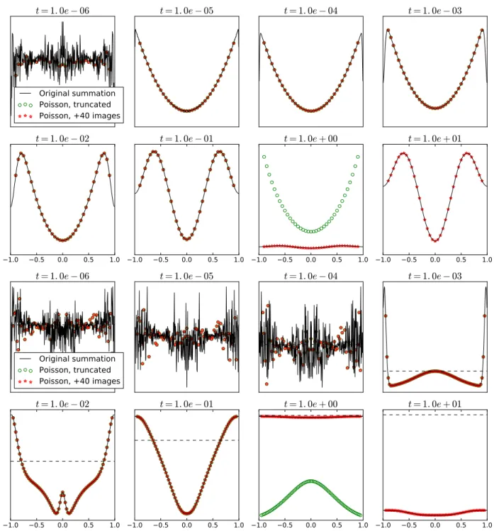
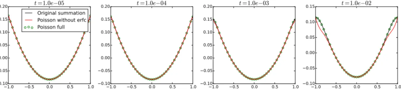
The Poisson summation shows the structure of the pointwise moment

T

(y, t)

at short time can

be interpreted as a lattice of scaled heat kernels

G(x

−

x

, t), with lattice

{x

= 2k

−

1, k

∈

Z

}.

With this in mind, a formal approach to the short time for general cross section can be formed.

We demonstrate this in the channel and will generalize to generic domain after. We would like a

short time approximation for the problem

∂T1

∂t

−

∂

∂y

T

=

u(y),

∂T1

∂y

y=±1

= 0,

T

(y,

0) = 0.

(3.32)

Start with a generic time expansion of the first moment

T1

(y, t)

and seek appropriate coefficients:

T

(y, t)

∼

a

(y)t

+

a

(y)

t

2

.

(3.33)

Substitution into the Aris equation and matching in powers of

t

gives

a

=

u,

a

=

−

2

∂y2

u

=

const.

(3.34)

However, this solution violates the conservation of

R

T

dy

required of the full solution:

Z

∂T1

∂t

−

Z

∂

∂y

T1dy

=

Z

udy

d

R

−1

T

dA

dt

−

h

∂T

∂

y

i

= 0

⇒

d

R

T

dy

dt

= 0,

whereas

d

dt

Z

a

t

+

a

t

/2

dy

=

Z

u

+ (−

∂

∂y

u)t

dy

= 2(−

∂

∂y

u)t

6= 0.

We seek a term

k(y)

to add which corrects the conservation requirement, but preserves the short

time dynamics, which are primarily advective:

t

2

Z

k(y) +

−

∂

∂y

u

dy

= 0

(3.36)

Z

k(y)

dy

=

Z

∂

∂y

u dy

=

h

∂u

∂y

i

.

(3.37)

While any choice of

k(y)

satisfying the integral requirement will restore conservation, analysis of

the channel solution reveals boundary layers which evolve characteristically like heat kernels for

t >

0, and in the limit

t

→

0, form a sequence converging to delta functions. Therefore, one choice

of correction in this small, but positive time regime would be

˜

k(y, t) =

c1G(y

−

1

, t) +

c2G(y

+ 1

, t) =

c1

e

−(y−₄1_t−)2

√

4πt

+

c2

e

√

4πt

.

(3.38)

For

t

1, each heat kernel integrates to

1

up to exponentially small corrections. Let

k(y) =

lim

˜

k(y, t), so

Z

k(y)dy

=

c1

+

c2

=

h

∂u

∂y

i

.

(3.39)

An appropriate choice is then setting

c

=

∂u

∂y

,

c

=

−

∂u

∂y

,

(3.40)

and if

u

= 1/3

−

y

, this gives

c1

=

c2

=

−2. Finally, we can verify the modified quadratic term

obeys conservation at short time (using

−∇

_u

_{= 2):}

t

2

Z

a2(y)dy

=

t

2

lim

Z

−

∂

∂y

u

−

2(G(y

−

1

−

_{, t) +}

_G(y

_{+ 1}

_{, t))}

dy

(3.41a)

=

t

2

[(1

−

(−1))(2)

−

2 [1 + 1]] = 0.

(3.41b)

The formal asymptotics at

t

= 0

are

T1

∼

u(y)t

+

−

∂

∂y

u

−

2(δ(y

−

1

−

) +

δ(y

+ 1

))

t