APPLICATION OF DIFFRACTIVE OPTICAL ELEMENT ON SPECTROSCOPY AND IMAGING
Zhenkun Guo
A dissertation submitted to the faculty at the University of North Carolina at Chapel Hill in partial fulfillment of the requirements for the degree of Doctor of Philosophy in the Department
of Chemistry in the College of Arts and Sciences.
Chapel Hill 2018
ABSTRACT
Zhenkun Guo: Application of Diffractive Optical Element on Spectroscopy and Imaging (Under the direction of Andrew Moran)
Diffractive optical elements (DOE) are optical components that manipulate light by diffraction, interference, and other phase control methods. The application of DOE in multi-dimensional spectroscopy could significantly reduce the efforts required for conducting
experiments and enhance the signal-to-noise ratio with high efficiency. In this dissertation, DOE-based two-dimensional resonance Raman spectroscopy was developed and implemented in two model systems, triiodide and myoglobin. This new technique uncovers new dimensions of information, which were not available with previous one-dimensional spectroscopy techniques. The DOE was also applied to the wide-field transient absorption microscopy. Conducting a large number of experiments simultaneously is possible in this configuration. Analysis of parallel measurements provides statistical information essential to comprehensively study heterogeneous samples.
Ligand binding and dissociation processes are crucial to the functions of heme proteins. The recovery of the protein matrix involves fast energy dissipation from the heme group to solvent, facilitated by the propionic acid side chains as an effective “gateway”. In this dissertation, we found that the propionic chains possess significant structural heterogeneity, which could be induced by the thermal fluctuation in geometries. It is interesting to consider whether the variation in conformation could relate to the vibrational cooling rate distributions.
Carrier diffusion is imaged in a perovskite film and crystal using a newly developed DOE-based wide-field transient absorption microscopy technique. The function of the instrument is illustrated with 41 parallel measurements conducted on methylammonium lead iodide
ACKNOWLEDGEMENTS
I would like to first thank my advisor, Dr. Andrew Moran, for his guidance and support throughout my doctoral studies. None of the work presented in this dissertation would have been possible without him. I would also like to thank past colleagues in the Moran group, including Dr. Brian Molesky, Dr. Paul Giokas and Andrew Ross for the help I got we I arrived at UNC and. I would like to specially express my deep gratitude to Dr. Brian, who trained me how to properly conduct optical experiments. Of course, I also thank my current colleagues, Thomas Cheshire, Olivia Williams, Ninghao Zhou, Michael Dinh and Daniel Bortolussi for their
contributions to the work. I thank my undergraduate academic/research advisor at the University of Science and Technology of China, Dr. Qun Zhang, for initially displaying the charm of
TABLE OF CONTENTS
LIST OF TABLES ... xiii
LIST OF FIGURES ... xiv
LIST OF ABBREVIATIONS AND SYMBOLS ... xxix
CHAPTER 1. INTRODUCTION ... 1
Applications of Diffractive Optical Elements ... 1
Application of Diffractive Optical Elements in Spectroscopy and the Development of Two-Dimensional Resonance Raman Spectroscopy ... 3
Coherent Reaction Mechanism in Triiodide Photo Dissociation ... 6
Structural Heterogeneity and Vibrational Energy Exchange in Myoglobin ... 9
Application of Diffractive Optical Element in Transient Absorption Microscopy ... 13
Carrier Diffusion in Organic Halide Perovskite Single Crystals and Thin Films ... 15
Dissertation Content... 17
REFERENCES ... 19
CHAPTER 2. METHODS AND INSTRUMENTATION ... 31
Introduction ... 31
Basics of Diffractive Optical Elements... 32
2.2.1. Principles of Diffracted Lights ... 32
2.3.1. Spectral Broadening of Femtosecond Pulses Using
Hollow-Core Fibers ... 38
2.3.2. White Light Generation by Filamentation in a Noble Gas ... 41
Principles of Nonlinear Spectroscopy ... 44
Third-Order Nonlinear Spectroscopy ... 48
2.5.1. Transient Absorption Spectroscopy ... 48
2.5.2. Four-Wave-Mixing Spectroscopy and Transient Grating Spectroscopy ... 51
Fifth-Order Nonlinear Spectroscopies ... 56
2.6.1. Diffractive Optics-Based Six-Wave-Mixing ... 56
2.6.2. Femtosecond Stimulated Raman Spectroscopy ... 60
2.6.3. Femtosecond Stimulated Raman Spectroscopy by Six-Wave-Mixing... 62
Multiplex Wide-Field Transient Absorption Spectroscopy ... 66
Summary ... 71
REFERENCES ... 72
CHAPTER 3. ELUCIDATION OF REACTIVE WAVEPACKETS BY TWO-DIMENSIONAL RESONANCE RAMAN SPECTROSCOPY ... 80
Introduction ... 80
2DRR Spectra Simulated for a Reactive Model System ... 82
3.2.1. Model Hamiltonians ... 83
3.2.2. Response Functions ... 86
3.2.3. Calculated 2DRR Spectra ... 91
Experimental Methods ... 93
3.3.1. Conducting 2DRR Spectroscopy with a Five-Beam Geometry ... 93
3.3.2. Conducting 2DRR Spectroscopy with a Three-Beam Geometry ... 96
Experimental Results ... 98
3.4.1. Third-Order Stimulated Raman Response ... 98
3.4.2. 2DRR Response of The Diiodide Photoproduct ... 99
3.4.3. 2DRR Cross Peaks Between Triiodide and Diiodide ... 101
3.4.4. Summary of 2DRR Signal Components ... 104
Nonequilibrium Correlation Between Reactants and Products ... 106
Concluding Remarks ... 111
Supplemental Information ... 112
3.7.1. Vibrational Hamiltonians ... 112
3.7.2. Two-Dimensional Resonance Raman Signal Components ... 114
REFERENCES ... 117
CHAPTER 4. FEMTOSECOND STIMULATED RAMAN SPECTROSCOPY BY SIX-WAVE MIXING ... 122
Introduction ... 122
Experimental Methods ... 126
4.2.1. Laser Pulse Generation ... 126
4.2.2. Laser Beam Geometries ... 128
4.2.3. Signal Detection ... 130
4.2.4. Sample Handling ... 131
Signal Processing ... 131
4.3.1. Algorithm ... 131
4.3.2. Adequate Suppression of the Broadband Response ... 136
4.3.3. Summary of Technical Issues Involved in Signal Processing ... 138
4.4.3. Relative Signs of Third- and Fifth-Order Signals ... 144
4.4.4. Dynamic Line Shapes of FSRS Signals Obtained by Six-Wave Mixing... 147
Theoretical Analysis of Relative Magnitudes of Resonant FSRS Signals and Cascades ... 151
4.5.1. Background ... 152
4.5.2. Response Functions ... 153
4.5.3. Model Calculations ... 157
Concluding Remarks ... 160
Supplemental Information ... 161
4.7.1. Direct Fifth-Order Signal Field ... 161
4.7.2. Cascaded Third-Order Signal Field ... 164
4.7.3. Distinguishing the Broadband and FSRS Responses ... 167
REFERENCES ... 169
CHAPTER 5. TWO-DIMENSIONAL RESONANCE RAMAN SPECTROSCOPY OF OXYGEN- AND WATER-LIGATED MYOGLOBIN ... 174
Introduction ... 174
Experimental Methods ... 178
5.2.1. Sample Preparation ... 178
5.2.2. Spectroscopic Measurements... 178
Simulations of 2DRR Spectra ... 181
5.3.1. Signatures of Inhomogeneous Broadening in 2DRR Spectra... 182
5.3.2. Signatures of Anharmonicity in 2DRR Spectra ... 184
5.3.3. Predicted 2DRR Spectrum of Myoglobin ... 187
Results and Discussion ... 189
5.4.2. Analysis of Spectral Line Shapes ... 195
5.4.3. Computational Analysis of Line Broadening Mechanism... 197
5.4.4. Implications for the Vibrational Cooling Mechanism ... 201
Concluding Remarks ... 202
Supplemental Information ... 203
5.6.1. Response Function ... 203
5.6.2. Anharmonic Vibrational Hamiltonian ... 206
5.6.3. Parameters Used in the Model ... 208
REFERENCES ... 210
CHAPTER 6. IMAGING CARRIER DIFFUSION IN PEROVSKITES WITH A DIFFRACTIVE OPTIC-BASED TRANSIENT ABSORPTION MICROSCOPE ... 217
Introduction ... 217
Experimental Methods ... 219
6.2.1. Sample Preparation ... 219
6.2.2. Transient Absorption Microscopy ... 220
Signal Processing ... 223
Results and Discussion ... 225
Conclusion ... 229
REFERENCES ... 231
CHAPTER 7. CONCLUDING REMARKS... 235
REFERENCES ... 239
APPENDIX A: SUPPLEMENT TO “ELUCIDATION OF REACTIVE WAVEPACKETS BY TWO-DIMENSIONAL RESONANCE RAMAN SPECTROSCOPY” ... 244
A.2. Dominance of the Direct 2DRR Response Over Third-Order
Cascades ... 251
A.3. References ... 254
APPENDIX B: SUPPLEMENT TO “FEMTOSECOND STIMULATED RAMAN SPECTROSCOPY BY SIX-WAVE MIXING” ... 256
B.1. Derivation of Formula for Direct Fifth-Order Signal Field ... 256
B.2. Derivation of Formula for Third-Order Cascaded Signal Field ... 264
B.2.1. Direct Coherent Stokes Raman Scattering (CSRS) Signal Field Obtained with the Phase Matching Condition k3-k4+k5 ... 265
B.2.2. Cascades with Intermediate Phase-Matching Conditions k1 -k2+k5 and k3-k4+k5 ... 267
B.3. References ... 272
APPENDIX C: SUPPLEMENT TO “TWO-DIMENSIONAL RESONANCE RAMAN SPECTROSCOPY OF OXYGEN- AND WATER-LIGATED MYOGLOBIN” ... 273
C.1. Signatures of Anharmonicity in Time-Frequency Representation of 2DRR Signal ... 273
C.2. Fluctuations in the Geometries of the Propionic Acid Side Chains Produced with Molecular Dynamics Simulations and an Ab Initio Map ... 276
C.3. References ... 278
APPENDIX D: SUPPLEMENT TO “IMAGING CARRIER DIFFUSION IN PEROVSKITES WITH A DIFFRACTIVE OPTIC-BASED TRANSIENT ABSORPTION MICROSCOPE” ... 279
D1. SEM Image of Perovskite Film ... 279
D2. SEM Image of Perovskite Single Crystal ... 279
LIST OF TABLES
Table 3.1. Parameters of Model Used to Compute 2DRR Spectra ... 91
Table 4.1. Parameters of Theoretical Model ... 166
Table 4.2. Wavevector Mismatch in the Five-Beam Geometry ... 167
Table 4.3. Wavevector Mismatch in the Four-Beam Geometry ... 167
Table 5.1. Parameters of Theoretical Model for System with Two Vibrational Modes ... 208
Table 5.2. Parameters of Model Based on Empirical Fit of Spontaneous Raman Signals ... 209
Table B1. Wavevector Mismatch in the Five-Beam Geometry ... 268
Table B2. Wavevector Mismatch in the Four-Beam Geometry ... 269
Table B3. Wavevector Mismatch in a (Hypothetical) Three-Beam Geometry ... 269
Table D1. Diffusion Coefficient D0 ... 280
Table D2. Density-Independent Relaxation Time τ1 ... 281
Table D3. Two-Body Relaxation Time τ2 ... 281
LIST OF FIGURES
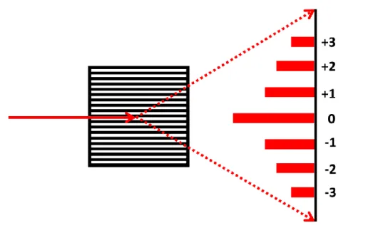
Figure 1.1. A simple grating made by closely separated periodical slits. The incoming light can be diffracted into different orders. For a transmissive grating, the 0th order will be the directly transmitted light. The angle between diffraction orders and the intensity distributions can be modulated by adjusting the slit
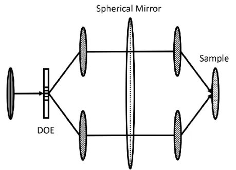
spacing and width. ... 2 Figure 1.2. A DOE is used to generate replicas of the incoming laser pulse in
both intensity and phase. The ovals represent a snapshot of the spatial pulse envelopes as they propagate through the optical system. One feature of using a DOE is that the pulse fronts are parallel in space and can entirely overlap with each other when focused on the sample (i.e., pulse front tilt is eliminated
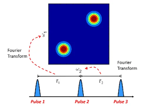
regardless of crossing angle). ... 4 Figure 1.3. An example of 2D Fourier transform vibrational spectroscopy.
Typically, two time intervals are built by three pulses, and the measured signal oscillates in both delays, 1 and 2. Fourier transforms of the time-domain vibrations result in peaks in the frequency domain, as shown in the figure. Vibrations in the 1 (2) dimension correspond to the signal in 1(2) in the 2D
Fourier transform. ... 5 Figure 1.4. Photo-dissociation process of triiodide after excitation. An excited
state wavepacket is initiated at the excited electronic state by photo-excitation, where the steep gradient of the potential energy surface drives the motion of the wavepacket along the symmetric stretch coordinates. Dissociation of triiodide yields a diiodide ion and a free iodine atom. This entire process occurs in approximately 300 fs, at the same time scale of the period of triiodide’s symmetric stretch. The non-equilibrium geometry of the reactant can have an influence on the vibrational coherence in the products. 2DRR with reactant evolution in one dimension and product evolution in the other can be used to
reveal such effects. ... 8 Figure 1.5. Structure of myoglobin in water. Green spheres represent the
porphyrin active site, while red spheres represent bonded oxygen. The propionic acid chains are circled in red and can form hydrogen bonds with water molecules. These side chains are the primary energy dissipation channel after ligand
dissociation. ... 10 Figure 1.6. Signatures of homogeneous and inhomogeneous line broadening
mechanisms in 2DRR spectra. The inhomogeneously broadened signal is
line broadening mechanisms are indistinguishable in one-dimensional Raman
spectroscopies. ... 12 Figure 1.7. The signals are measured simultaneously from 41 different spots on
the sample surface, as shown in the figure. A DOE splits the incoming pump beam into 41 segments with equal intensity and parallel aligned wave-fronts. These beams are focused onto many spots on the sample because of the different diffraction angles. Since the probe is focused to a much larger area covering all the spots, the TA response can be measured simultaneously from all 41 positions.
Statistical information is available after only a single experiment. ... 15 Figure 2.1. Illustration of the symbols used in Equation 2.1 and Equation 2.2. ris
the distance between a point in the object plane and a point in the detection plane,
2 2 2
( ) ( )
r= X −x + Y−y +Z
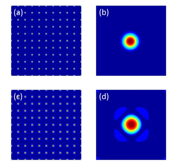
... 32 Figure 2.2. A simple simulation to show the distortion introduced by the
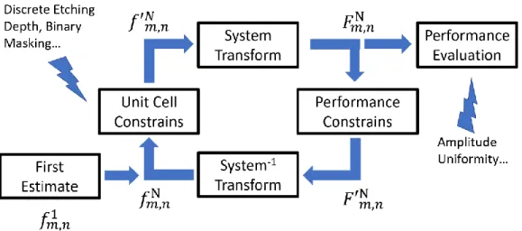
quantized phase and binary amplitude modulations limitations imposed by the lithography etching technique. (a) is the desired diffraction pattern and (b) is one diffraction order (unit cell) of the desired pattern. In the simplest case, one diffraction order is given by a two-dimensional Gaussian function. (c) and (d) show the diffraction pattern and unit cell obtained by DOE designed through the direct inverse Fourier transform method. The phase is quantized to eight different levels (0, , ,3 , ,5 ,3 ,7
8 4 8 2 8 4 8
) and the amplitudes modulation is binary
(0,1). Distortion of the unit cell pattern is clearly introduced. ... 36 Figure 2.3. A typical iterative algorithm to optimize the diffractive optical
element design. ... 38 Figure 2.4. The effect of self-phase modulation in a hollow-core fiber. The plot
assumes a Gaussian pulse propagating through isotropic media with positive n2. The frequency of the pulse red-shifts at the rising edge (i.e., t0) and blue-shifts at the falling edge (i.e., t0). The frequency does not shift (i.e,. =0) at the
pulse envelope maximum. ... 40 Figure 2.5. An illustration of the focusing–defocusing cycles induced by the
competing self-focusing and plasma defocusing. The solid curves indicate the diameter of the laser beam. The filament is built by a large number of these
cycles, and the filament length is the distance covered by the cycles. ... 43 Figure 2.6. In a third-order nonlinear spectroscopy, two Feynman diagrams for a
Figure 2.7. These three Feynman diagrams illustrate examples of GSB, ESE, and ESA measured by transient grating and transient absorption spectroscopy.
Although not all terms contributing to these two techniques are plotted in the figure, all response function terms measured can be classified into these three
categories. ... 51 Figure 2.8. Typical transient grating experiment geometry. Two time-coincident
pump pulses arrive at the sample first. Then, after some waiting time τ, the probe pulse arrives and generates the signal. The signal is emitted in a different direction from all incoming laser beams determined by the phase match condition.
Therefore, the measurement is background free and no optical chopper is
necessary. ... 52 Figure 2.9. The concept of grating formation in transient grating measurements.
Two time-coincident pump beams with different wavevectors cross in the sample at an angle 2𝜃 and interfere to form a population grating. After a delay, the probe arrives and is scattered off the grating in the signal directionksig = − +k1 k2 k3,
where k1 and k2 are the pump beams and k3 is the probe. ... 52
Figure 2.10. An illustration of how the interferometric detection method magnifies the signal and why the phase fluctuation has significant influence on the measured signal. (a) The real parts of the electronic fields are shown in the time domain as a summation over all frequencies. The reference (Ref) field is five times stronger than the signal. The disturbance in the optical path on the times scale of 0.7 fs could shift the 400 nm light by π/2, as indicated by the red lines. (b) The measured signal is the square of the time-integrated sum between the
reference field and the signal. Fringes are generated by the interference between the reference field and the signal. If the reference field varies by 0.7 fs in optical
path, it may cause a 25% reduction of peak intensity. ... 54 Figure 2.11. A typical geometry for the diffractive optical element (DOE)-based
transient grating setup. Two beams are focused onto the DOE and split into ±1 diffraction orders. A spherical mirror reflects and focuses the four beams. Beams 1 and 2 induce the population grating, and the transient grating diffracts beam 3 (the probe). The diffracted signal beam is collinear with beam 4, which is an attenuated reference field for heterodyne detection. A typical interferometric
signal measured on the spectrometer is shown. ... 56 Figure 2.12. A diffractive optic-based four-beam interferometer used to measure
the six-wave-mixing signal in Chapter 3. Compared to the geometry used in the four-wave-mixing transient grating in Figure 2.11, an additional pump beam arrives before the formation of population grating. A nonequilibrium state of the sample molecules can be prepared before measuring the transient grating signal. The signal emits in the same direction as in the transient grating case, collinear to
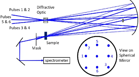
Figure 2.13. A diffractive optic-based interferometer with five-beam geometry is used to measure the six-wave-mixing signal in Chapter 3. The three incoming beams are split into -1, 0, and +1 diffraction orders with even intensity
distribution. A mask on the spherical mirror blocks beams not marked with numbers. Beams 1 and 2 firstly excite the sample and produce a population grating. After a delay τ, beams 3 and 4 arrive and re-excite the sample from a prepared nonequilibrium state. These four beams generate a two-dimensional crossing grating. The last, beam 5, is diffracted by this grating in the same
direction as beam 6, the attenuated reference field, for heterodyne detection. ... 58 Figure 2.14. Population grating generated by the six-wave-mixing geometry
demonstrated in Figure 2.13. A 266 nm deep UV laser beam generates the
patterns, as described in Chapter 3. The angle between 1 orders of the diffracted light is 6.1 degrees. The figures represent the views observed from a direction perpendicular to the sample surface. (a) The population grating formed by the first two pumps, beams 1 and 2. (b) The population grating formed by all four pumps, beams 1 through 4. These gratings are not moving due to the degenerate condition
for all beams. ... 60 Figure 2.15. (a) A schematic representation of time-resolved femtosecond
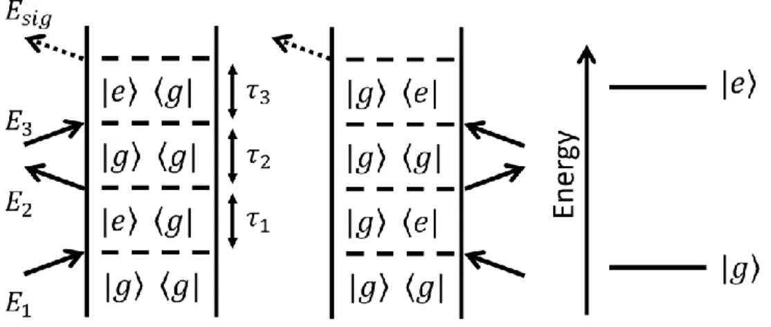
stimulated Raman spectroscopy (FSRS). A femtosecond actinic pump pulse initiates photochemistry by promoting the system to an excited electronic state first. Then, the combination of a Raman pump pulse and a Stokes probe pulse induces the emission of the stimulated Raman signal. (b) The sequence of the actinic pump, the Raman probe, and the Stokes probe. (c) An energy diagram illustrates the key to femtosecond time precision. The actinic pump promotes the systems into an electronically excited state with two field-matter interactions. Then, the vibrational coherence n n+1 is driven by the time-overlapped Raman pump and Stokes probe pulses from a prepared nonequilibrium state. The signal can actually emit anytime under the time-envelope of the Raman pump with the second field-matter interaction while the vibrational coherence is dephasing. The time precision depends on the time convolution between the actinic pump and the
probe. ... 61 Figure 2.16. (a) The five-beam geometry used for FSRS by six-wave-mixing
(6WM) experiments in this dissertation. This design is much like the
Figure 2.17. Views of gratings from the direction perpendicular to the sample surface. (a) The static grating formed by the time coincident actinic pump beams, beam 1 and 2 in the five-beam geometry experiment. However, because the first two field-matter interactions are induced by the same beam in the four-beam geometry, no grating is formed. (b) In both the four- and five-beam experiments, a dynamic population grating is generated by the Raman pump and Stokes beams because of the difference in wavelength. The interference pattern moves down and to the right. (c) In the five-beam geometry, the overall FSRS grating is the summation of the two gratings in (a) and (b) and moves down and to the left. In both four- and five-beam geometries, the moving direction of the overall
population grating is opposite to the signal propagating direction. Therefore, the
Doppler shifts could induce a red-shift in frequency. ... 65 Figure 2.18. A schematic illustration of the all-reflective 4F setup. A grating
disperses the incoming broadband or super-continuum white light into a wide range of angles. The dispersed light is then focused by a concave spherical mirror to a flat mirror where different colors are spatially separated. A slit can be placed right in front of the flat mirror to select the desired wavelength range, then the flat mirror reflects the selected portion backward to the concave mirror and the
grating. The distance between the concave mirror and grating as well as the distance between the concave mirror and the flat mirror are equal to the focus length of the concave mirror. The final output beam has the same beam profile as
the incoming beam with frequencies selected by the slit. ... 67 Figure 2.19. Transient absorption microscopy experiments are conducted with a
diffractive optic-based wide-field microscope. (a) A diffractive optic is used to generate a 41-point array of pump beams, which focus at different places on the sample. (b) The diffractive optic produces a 41-point matrix of laser beams, which all possess equal intensities. (c) A counter-propagating pump and probe beams are focused to full width at half maximum (FWHM) spot sizes of 0.73 and 150 μm on
the sample surface, respectively. ... 68 Figure 2.20. Frequency-resolved transient absorption spectrum was measured on
a single spot of the two-dimensional perovskite film. The probe was scanned from 605 nm to 790 nm and resolved exciton peaks for quantum confined
two-dimensional layers. ... 70 Figure 3.1. Linear absorbance spectra of triiodide and diiodide in ethanol. The
absorbance spectrum of triiodide is directly measured, whereas that of diiodide is derived from Ref. 35 because it is not stable in solution. Diiodide is probed on the picosecond time scale in the present work. The electronic resonance frequencies associated with this nonequilibrium state of diiodide are likely red-shifted from
those displayed above. ... 83 Figure 3.2. Feynman diagrams associated with dominant 2DRR nonlinearities.
states of the triiodide reactant, whereas 𝑝 and 𝑝 ∗correspond to the diiodide photoproduct. Vibrational levels associated with these electronic states are specified by dummy indices (𝑚, 𝑛, 𝑗, 𝑘, 𝑙, 𝑢, 𝑣, 𝑤). Each row represents a different class of terms: (i) both dimensions correspond to triiodide in terms 1-4; (ii) both dimensions correspond to diiodide in terms 5-8; and (iii) vibrational resonances of triiodide and diiodide appear in separate dimensions in terms 9-12. The intervals shaded in blue represent a non-radiative transfer of vibrionic coherence from
triiodide to diiodide. ... 88 Figure 3.3. Absolute values of 2DRR spectra computed using (a) the sum of
terms 1-4 in Equation 3.22. (b) the sum of terms 5-8 in Equation 3.23 and (c) the sum of terms 9-12 in Equation 3.24. The frequency dimensions, ω1 and ω2, are
conjugate to the delay times, τ1 and τ2 (see Figure 3.2). Signal components of the
type shown in panel (a) are generally detected in one-color experiments. Two-color 2DRR approaches are used to detect nonlinearities that correspond to panels (b) and (c) in this work. The peaks displayed in (c) are unique in that resonances
of the reactant and product are found in ω1 and ω2, respectively. ... 93
Figure 3.4. (a) Diffractive optic-based interferometer used to detect signal
components described by terms 5-8 in Figure 3.2. Each of the two 680-nm beams is split into −1 and +1 diffraction orders with equal intensities at the diffractive optic. The signal is collinear with the reference field (pulse 5) used for
interferometric signal detection. (b) The 340-nm pulse induces photodissociation and vibrational coherence in the diiodide photoproduct during the delay, τ1. The
time-coincident 680-nm pulses, 2 and 3, reinitiate the vibrational coherence in
diiodide during the delay, τ2. ... 94
Figure 3.5. (a) Pump-repump-probe beam geometry used to detect signal components described by terms 9-12 in Figure 3.2. (b) The first 400-nm pulse promotes a stimulated Raman response in the ground electronic state of the triiodide reactant during the delay, τ1. The second pulse induces photodissociation
of the non-equilibrium reactant, thereby giving rise to vibrational coherence in the diiodide photoproduct during the delay, τ2. Sensitivity to diiodide is enhanced by
signal detection in the visible spectral range. ... 97 Figure 3.6. (a) Transient absorption signals (in mOD) obtained for triiodide with
a 400-nm pump pulse and continuum probe pulse. (b) The coherent component of the signal is isolated by subtracting sums of 2 exponentials from the total signal presented in panel (a). (c) Fourier transformation of the signal between delay times of 0.1 and 2.5 ps shows that the vibrational frequency decreases as the detection wavenumber decreases. Dispersion in the vibrational frequency reflects sensitivity to high-energy quantum states in the anharmonic potential of
signal is isolated by subtracting sums of two exponentials from the total signal presented in panel (a). (c) The two-dimensional Fourier transformation of the signal in panel (b) reveals resonances in the upper right and lower left quadrants. This pattern of 2DRR resonances is consistent with calculations based on terms
5-8 (see Figure 3.3), which this experiment is designed to detect. ... 100 Figure 3.8. 2DRR data are obtained using the two-color approach described in
Figure 3.5. Each column corresponds to a different detection wavenumber: 22500 cm-1 (444 nm) in column 1; 21000 cm-1 (476 nm) in column 2; 19500 cm-1 (513
nm) in column 3; 18000 cm-1 (555 nm) in column 4. (a)-(d) Total pump-repump-probe signal in mOD. (e)-(h) Coherent parts of the pump-repump-pump-repump-probe signals displayed in the first row. (i)-(l) 2DRR spectra are generated by Fourier
transforming the signals shown in the second row in delay ranges, 𝜏1 and 𝜏2, between 0.15 and 2.0 ps. The data show that peaks in the upper left and lower right quadrants emerge as the detection wavenumber becomes off-resonant with triiodide. Signals acquired at detection wavenumbers above 21,000 cm-1 (476 nm) are dominated by stimulated Raman processes in the ground electronic state of triiodide (terms 1-4). In contrast, signals acquired at detection wavenumbers below 19,500 cm-1 (513 nm) are consistent with terms 9-12, where vibrational
resonances in 𝜔1 and 𝜔2 correspond to triiodide and diiodide, respectively. ... 102 Figure 3.9. Summary of 2DRR experiments conducted on triiodide: (a) the
response of triiodide was detected in both dimensions in Reference 26; (b) the response of the diiodide photoproduct is detected in both dimensions (see Figure 3.7); (c) the response of triiodide and diiodide are detected in separate dimensions (see Figure 3.8). Blue and red laser pulses represent wavelengths that are
electronically resonant with triiodide and diiodide, respectively. ... 105 Figure 3.10. 2DRR response of triiodide in ethanol with a detection wavenumber
of 19,500 cm-1 (513 nm). (a) Resonances in all four quadrants of the 2DRR
spectrum signify cross peaks between triiodide (in 𝜔1) and diiodide (in 𝜔2). (b) Quantum beats in the Raman spectrum of diiodide are observed when the 2DRR spectrum in panel (a) is inverse Fourier transformed with respect to 𝜔1. (c) Oscillations in the mean vibrational frequency are analyzed using Equation 3.6. Such oscillatory behavior suggests that the vibrational coherence frequency of
diiodide is sensitive to vibrational motions of triiodide in the delay time, 𝜏1. ... 106 Figure 3.11. The sequence of events associated with the 2DRR signals shown in
Figure 3.10. Rab and Rbc denote the two bond lengths in triiodide. (a) The first
pulse initiates a ground state wavepacket in the symmetric stretching coordinate. Force is accumulated when both bond lengths increase during the electronic coherence induced by the first laser pulse. (b) Wavepacket motion on the ground state potential energy surface is detected in the delay between the pump and repump laser pulses, 𝜏1. (c) Photodissociation of triiodide is initiated from a nonequilibrium geometry by the repump laser pulse. The Raman spectrum of
Figure 3.12. Correlation between the vibrational wavenumber of the diiodide photoproduct and the pair of bond lengths in the triiodide reactant, Rab=Rbc, is
illustrated by analyzing the dynamics in the mean vibrational coherence
frequency, vib
( )
1 , shown in Figure 3.10(c). The delay time, 𝜏1, is converted into the position of the wavepacket in the symmetric stretching coordinate using the model presented in Figure 3.11. Each revolution of the spiral corresponds to 300 fs. The wavepacket oscillates around the equilibrium bond length until vibrational dephasing is complete. The diagonal slant in the spiral suggests that a bond length displacement of 0.1 Å in triiodide induces a shift of 6.8 cm-1 in thevibrational coherence frequency of diiodide. ... 110 Figure 4.1. (a) A five-beam FSRS geometry is used in this work to eliminate the
portion of the background associated with residual Stokes light and third-order nonlinearities. The color code is as follows: the actinic pump is green, the Raman pump is blue, and the Stokes pulse is red. (b) Relaxation dynamics are probed in the delay between the actinic pump and Stokes pulses,
1. The fixed time delay,2
, is used to suppress a broadband pump-repump-probe response. ... 124Figure 4.2. Spectra of the actinic pump (green), Raman pump (blue), and Stokes pulses (red) are overlaid on the linear absorbance spectrum of metmyoglobin in
aqueous buffer solution at pH=7.0. ... 127 Figure 4.3. (a) Diffractive optic-based interferometer used for FSRS
measurements. The transparent fused silica window delays pulse 3 by 290 fs with respect to pulse 4 (delay
2 in Figure 4.1). (b) A five-beam geometry is used to detect the FSRS signal in the background-free direction, k1-k2+k3-k4+k5. (c) TheFSRS signal is also radiated in the direction, k1-k2+k3-k4+k5 in the four-beam
geometry; however, the wavevectors k1 and k2 cancel each other, so the signal is
radiated in the same direction as a four-wave mixing signal, k3-k4+k5. In the
four-beam geometry, the FSRS signal corresponds to the difference between signals measured with and without the actinic pump beam (beam 1,2). Beams represented with solid circles reach the sample, whereas those represented with open circles are blocked with a mask. The same color code is applied in all panels (Raman
pump is blue, actinic pump is green, Stokes beam is red). ... 128 Figure 4.4. (a) This six-wave mixing signal for metMb is obtained in the
response, which is dominant at earlier times. (d) The absolute value of the FSRS
spectrum is obtained by Fourier transformation of the filtered signal in panel (c). ... 134 Figure 4.5. Molecular structure of iron protoporphyrin-IX. ... 135 Figure 4.6. This six-wave mixing signal for metMb is obtained in the five-beam
FSRS geometry with
2=420 fs The panels (a)-(d) are defined in the same way as those in Figure 4.4. The vibrational frequencies obtained in this measurement differ by less than 10 cm-1 from those found in Figure 4. This difference is 5 times less than the bandwidth of the Raman pump pulse (i.e., intrinsic frequencyresolution). The vibrational line widths are roughly 25% less than those shown in Figure 4.4. This decrease in the line width with increasing delay,
2, is consistentwith the theory outlined in Section 4.5. ... 136 Figure 4.7. Signal intensities corresponding to the vibrational resonance at 1370
cm-1 are plotted versus incident pulse energies. In the first row, the signal,
( )
( )
FSRS BB
E E , is plotted versus energies of (a) actinic pump, (b) Raman pump, and (c) Stokes beams. In the second row, the signal, EFSRS
( )
, is plotted versus energies of the (d) actinic pump, (e) Raman pump, and (f) Stokes beams. Pulse energies associated with the actinic and Raman pump represent sums for the respective pairs of beams at the sample position (i.e.,beams 1 and 2 or beams 3 and 4). The functional forms used to fit the data (red lines) are indicated in the respective panels. These data validate the signal processing algorithm described in Section 4.3 and confirm that saturation of the optical response is negligible inthese ranges of the pulse energies. ... 140 Figure 4.8. (a) FSRS signal intensities associated with the vibrational resonance
at 1370 cm-1 are plotted versus the optical density of the solution in a 0.5-mm path length. The functions, Idirect( )5
( )
C and Icascade( )
C , illustrate how the data compare to the concentration dependence predicted for (red) the direct fifth-order signal and (blue) third-order cascades. The functions, Idirect( )5( )
C and Icascade( )
C , aremultiplied by constants to overlay them with the measured signal intensities. (b) Dynamics in the peak intensity at 1370 cm-1 are experimentally indistinguishable at various sample concentrations. (c) Signal intensities are overlaid at the highest
and lowest concentrations to illustrate the range in the data quality. ... 143 Figure 4.9. (a) Signals acquired in the four-beam geometry at various delay times
In contrast, third-order cascades would induce an increase in the total signal intensity, because such nonlinearities are in-phase with the third-order response. (c) Oscillatory features associated with the vibrational resonances are phase-shifted by approximately 180º in third- and fifth-order measurements (these are
magnified views of the data in panels (a) and (b)). ... 145 Figure 4.10. (a) Contour plot of signal field magnitude, EFSRS , obtained for
metMb in the five-beam geometry. (b) Temporal decay profiles for vibrational resonances detected in FSRS response. (c) Distributions of relaxation times for various resonances are obtained using the maximum entropy method. (d)-(f) FSRS signal field magnitudes are overlaid with fits conducted using the
maximum entropy method. ... 148 Figure 4.11. Laser beam geometries used to acquire (a) stimulated Raman and (b)
transient grating signals shown in (c) and (d), respectively. Beams represented with solid circles reach the sample, whereas those represented with open circles are blocked with a mask. (e) The two four-wave mixing signals are combined to simulate the cascaded response. (f) Unlike the FSRS signals plotted in Figure 4.10, all vibrational resonances decay with indistinguishable temporal profiles in the simulated cascade. Signal magnitudes for the 670 and 1370-cm-1 vibrational
resonances are shown as examples. ... 150 Figure 4.12. Double- sided Feynman diagrams associated with four classes of
terms in the FSRS response function. The terms are classified according to
whether or not they evolve in ground or excited state populations during the delay times,
1 and
2. The laser pulses associated with each field-matter interactionare indicated in the figure in the same color-code employed in Figure 4.2. ... 153 Figure 4.13. Feynman diagrams associated with the nonlinearities on the two
molecules involved in third-order cascades with intermediate phase-matching conditions (a) k1-k2+k5 and (b) k3-k4+k5. Field-matter interactions are
color-coded as follows: actinic pump is green; Raman pump is blue; Stokes is red; cascaded signal field is red; the field radiated at the intermediate step in the
cascade is purple. ... 155 Figure 4.14. Absolute values of signal spectra computed using the models
presented in appendices A and B and the parameters in Tables 4.1 and 4.2. The system possesses a single 1370-cm-1 harmonic mode with a displacement of 0.35 (a reasonable estimate for metMb).42 The frequency of the actinic pump pulse is set equal to the electronic resonance frequency,
AP =
eg. This calculationassumes that the five-beam geometry is employed (cascades are 4 times weaker in
Figure 4.15. (a) The ratio, ( )5
( ) / ( )
cas t direct t
E E , is computed for a system with a single harmonic mode under electronically resonant conditions,
AP =
eg.Theratio is computed at the value of the Raman Shift equal to the mode frequency (i.e., at the peak of the vibrational resonance). (b) The ratio,
( )5
( ) / ( )
cas t direct t
E E , is computed for a 670- cm-1mode at various dimensionless displacements and detuning factors,
AP−
eg. (c) The ratio,( )5
( ) / ( )
cas t direct t
E E , is computed for a 1370-cm-1 mode at various
dimensionless mode displacements and detuning factors,
AP−
eg. Boxes aredrawn in the regions of the plots relevant to myoglobin in panels (b) and (c). ... 160 Figure 4.16. (a) Examples of Feynman diagrams associated with the desired
FSRS and undesired broadband responses. The indices, g and
e
, represent the ground and excited electronic states, whereas dummy indices (m
,n
,k,l,u
, andv
) denote vibrational levels. Green, blue, and red arrows represent the actinic pump, Raman pump, and Stokes pulses, respectively. (b) The FSRS component of the response of metMb increases as the delay
2 increases (the delay,
1, is 0.5 pshere). This effect can be understood by inspection of the Feynman diagrams,
which suggest that the FSRS response will increase as the delay
2 increases. ... 168 Figure 5.1. (a) A four-beam FSRS geometry is used in this work to eliminate theportion of the background associated with residual Stokes light and a pump-probe response. The color code is as follows: the actinic pump is green, the Raman pump is blue, and the Stokes pulse is red. (b) Vibrational coherences in
1 are resolved by numerically Fourier transforming the signal with respect to the delay time. Time-coincident Raman pump and Stokes pulse then initiate a second set of vibrational coherences, which are resolved by dispersing the signal pulse on an array detector. The fixed time delay,
2, is used to suppress the broadbandpump-repump-probe response of the solution. ... 176 Figure 5.2. Laser spectra are overlaid on the linear absorbance spectra of (a)
metMb and (b) MbO2 in aqueous buffer solution at pH=7.0. ... 179
Figure 5.3. Diffractive optic-based interferometer used for 2DRR measurements. The transparent fused silica window delays pulse 3 by 290 fs with respect to pulse 4 (delay 2 in Figure 5.1). A four-beam geometry is used to detect the signal radiated in the direction, k1-k2+k3-k4+k5; the wavevectors k1 and k2 cancel each
other. The 2DRR signal is obtained by measuring differences with and without the actinic pump (beam 1,2). Beams represented with solid circles reach the
Figure 5.4. 2DRR spectra computed for a pair of harmonic oscillators with inhomogeneous line broadening. The spectra are computed by combining Equations 5.1 and 5.23 with the parameters given in Table 5.1. The correlation parameter, , is set equal to (a) -0.75, (b) 0.0, and (c) 0.75. The diagonal peaks always exhibit correlated line shapes, whereas the orientations and intensities of
the off-diagonal peaks depend on the correlation parameter, . ... 184 Figure 5.5. 2DRR spectra computed with the anharmonic vibrational Hamiltonian
described in Section 5.7.2 and the parameters in Table 5.1. The diagonal cubic expansion coefficients are set equal to -5 (first row), 0 (second row), and 5 cm-1 (third row). The off-diagonal expansion coefficients are set equal to -5 (first column), 0 (second column), and 5 cm-1 (third column). The response of a harmonic system is shown in panel (e). These calculations suggest that
anharmonic coupling promotes intensity borrowing effects via the transformation of Franck-Condon overlap integrals from the harmonic to anharmonic basis set (see Equation 5.26). For many of the parameter sets, anharmonicity causes the intensity of the cross peak above the diagonal to increase relative to that of the
cross peak below the diagonal. This effect is most pronounced in the left column. ... 185 Figure 5.6. 2DRR spectrum of myoglobin computed using parameters obtain by
fitting spontaneous resonance Raman excitation profiles.67 The spectrum is
dominated by resonances on the diagonal. The most dominant cross peak is associated with the iron-histidine stretch (
1/ 2
c
=220 cm-1) and in-plane stretching mode (
2/ 2
c
=1356 cm-1). The spectra are computed by combiningEquation 5.23 with the parameters in Table 5.2. ... 189 Figure 5.7. Signals obtained for (a) metMb and (d) MbO2 in a FSRS-like
representation. At each point in
2, the incoherent baseline is generated using themaximum entropy method. Shown here are slices of the signals for (b) the 670-cm-1 mode of metMb and (e) the 370-cm-1 mode of MbO2. Coherent residuals are
obtained by subtracting incoherent MEM baselines from the total signals for (b) metMb and (e) MbO2. The coherent residuals are presented for (c) metMb and (f)
MbO2. ... 190
Figure 5.8. Molecular structure of iron protoporphyrin-IX. ... 191 Figure 5.9. Experimental 2DRR spectra for (a) metMb and (b) MbO2 are
generated by Fourier transforming the coherent residuals with respect to
1 at each point in
2 (i.e., at each pixel in CCD detector). For both systems, diagonal peaks are detected near 220, 370, 674, and 1356 cm-1 (close to 1373 cm-1 intwo-dimensional Gaussians with correlation parameters in panels (c) and (d) (see Equation 5.2). The parameter,
, ranges between the uncorrelated (
=0) and fully correlated (
=1) limits for diagonal peaks. A correlation parameter greater than 0 is a signature of inhomogeneous line broadening. In panels (e) and (f), the slope consistent with each correlation parameter is overlaid on the experimental data to offer an additional perspective. For both systems, the 370-cm-1 methylene deformation mode local to the propionic acid side chains exhibits the greatestamount of heterogeneity (wavenumber near 370 cm-1). ... 196 Figure 5.11. Dihedral angles associated with the propionic acid chains are
defined for the heme in (a) metMb and (d) MbO2. The vibrational frequency of
the methylene deformation mode local to the propionic acid side chains is computed as a function of the two dihedral angles for (b) metMb and (e) MbO2.
These ab initio maps are used to parameterize the vibrational frequencies
associated with molecular dynamics simulations. Segments of the trajectories for
vibrational frequencies are shown for (c) metMb and (f) MbO2. ... 199
Figure 5.12. Spectral densities of the methylene deformation modes obtained from molecular dynamics simulations. The spectral densities decay to less than 50% of the maximum values at frequencies corresponding to the fluctuation amplitudes (5.9 and 7.0 cm-1 for metMb and MbO
2). These calculations are
consistent with an intermediate line broadening regime. ... 201 Figure 6.1. Transient absorption microscopy experiments are conducted with a
diffractive optic-based, wide-field microscope. (a) A diffractive optic is used to generate an array of pump beams which focus at different places on the sample. (b) Array of 41 pump laser beams is focused onto the sample surface. (c) Counter-propagating pump and probe beams are focused to FWHM spot sizes of 0.7 and
150 μm, respectively. ... 220 Figure 6.2. Control experiments are conducted to establish a model for signal
processing. (a) The decay rate decreases with distance from the center of one of the pump beams because of the decrease in laser fluence. Transient absorption signals measured at 760 nm for the (b) film and (c) crystal exhibit square root
dependencies on the fluence of the pump beam (pump is at 570 nm). ... 222 Figure 6.3. Transient absorption spectra measured for the perovskite (a) film and
(b) crystal with a 570-nm pump wavelength. Imaging for both systems is
conducted with at probe wavelength of 760 nm. ... 224 Figure 6.4. Transient absorption signals measured with 570-nm pump beam and
760-nm probe beam with a pump fluence of 40 μJ/cm2. Images measured for a
perovskite film at delay times of (a) 1 ps, (b) 500 ps, and (c) 1000 ps. Images measured for a perovskite single crystal at delay times of (d) 1 ps, (e) 500 ps, and (f) 1000 ps. The sizes of the signal spots expand as the delay time increases
Figure 6.5. Full-width-half-maximum spot widths measured for a
methylammonium lead iodide perovskite film (top row) and single crystal (bottom row). The data are fit with Equation 6.1 (blue line). These data suggest that
dynamics in the film and crystal are associated with fluence-dependent carrier
lifetimes and carrier diffusion, respectively... 227 Figure 6.6. Statistical analyses of fitting parameters for perovskite film and single
crystal: (a) diffusion coefficients, D0; (b) single-body relaxation rate, 1 1 −
; (c) two-body relaxation rate, 1
2
− . The uncertainty intervals represent two standard deviations. These data confirm the negligibility of carrier diffusion in the perovskite film. In contrast, expansion of the signal spots observed for the
perovskite crystal is dominated by carrier diffusion. ... 228 Figure A1. Fenyman diagrams associated with dominant 2DRR nonlinearities.
Blue and red arrows represent pulses resonant with triiodide and diiodide, respectively. The indices r and r* represent the ground and excited electronic
states of the triiodide reactant, whereas p and p* correspond to the diiodide photoproduct. Vibrational levels associated with these electronic states are specified by dummy indices (
m
,n
,j,k,l,u
,v
,w
). Each row represents a different class of terms: (i) both dimensions correspond to triiodide in terms 1-4; (ii) both dimensions correspond to diiodide in terms 5-8; (iii) vibrationalresonances of triiodide and diiodide appear in separate dimensions in terms 9-12. The intervals shaded in blue represent a non-radiative transfer of vibronic
coherence from triiodide to diiodide. ... 244 Figure A2. Comparison of signal phases obtained for third-order (pump-probe)
and fifth-order (pump-repump-probe) signals. (a) Pump-probe (delay of 0.5 ps) and pump-repump-probe (
1=
2=0.5 ps) signals have similar line shapes but opposite signs. This sign-difference suggests that the pump-repump-probe signal is dominated by the desired fifth-order nonlinearity (i.e., not third-order cascades). (b) Oscillations in pump-probe and pump-repump-probe signals are compared with signal detection at 20,000 cm-1 (500 nm). This is a slice of thepump-repump-probe signal in
2 with the delay,
1, fixed at 0 ps. A relative phase-shiftnear 180º suggests that the oscillatory component of the pump-repump-probe
signal is dominated by the direct fifth order nonlinearity.8 ... 253 Figure B1. Feynman diagrams associated with the direct fifth-order response. The
indices, g and
e
, represent the ground and excited electronic states, whereas dummy indices (m
,n
,k,l,u
, andv
) denote vibrational levels. Green, blue, and red arrows represent the actinic pump, Raman pump, and Stokes pulses,Figure B3. Feynman diagrams associated with the direct third-order CSRS response. The indices, g and
e
, represent the ground and excited electronic state, whereas dummy indices (m
,n
,k, and l) denote vibrational levels. Blueand red arrows represent the Raman pump and Stokes pulses, respectively. ... 265 Figure C1. Spectral components associated with oscillations of the mean
vibrational resonance frequencies computed with an anharmonic vibrational Hamiltonian. The diagonal expansion coefficients are set equal to -5 (first row), 0 (second row), and 5 cm-1 (third row). The off-diagonal expansion coefficients are set equal to -5 (first row), 0 (second row), and 5 cm-1 (third row). All amplitudes are normalized to the maximum found for the 400-cm-1 mode in the second row and first column. These calculations show that oscillations in the mean vibrational resonance frequencies occur primarily at the difference frequency in the harmonic system (see panel (e)). Anharmonicity increases the amplitude of oscillations at
the fundamental frequencies of the vibrations. ... 275 Figure C2. Distribution of dihedral angles for 5000 steps of the molecular
dynamics trajectory simulated for metMb. The equilibrium dihedral angles
associated with the propionic acid side chains (see Figure 5.11 in Chapter 5 of this
dissertation) are
L=81.3° and
R=81.1°. ... 276Figure C3. Distribution of dihedral angles for 5000 steps of the molecular dynamics trajectory simulated for MbO2. The equilibrium dihedral angles
associated with the propionic acid side chains (see Figure 5.11 in Chapter 5 of this
dissertation) are
L=94.4° and
R=109°. ... 277 Figure D1. Individual grains are observed in this SEM image of a perovskiteLIST OF ABBREVIATIONS AND SYMBOLS
1D one-dimensional
2D two-dimensional
3D three-dimensional
2DRR two-dimensional resonance Raman spectroscopy
4WM four-wave-mixing
6WM six-wave-mixing
absorption coefficient or a time constant used to suppress noise A linear scaling parameter or absorption
a lowering ladder operator or path length
†
a raising ladder operator
atm atmosphere
( )
,A z t real slowly varying amplitude envelope
Å angstrom
BBO beta barium borate
m
B Boltzmann population of level m
C concentration
c speed of light
°C Celsius temperature
. .
c c conjugate to the previous function CCD charge-coupled device image sensor
cm centimeter
CO carbon monoxide comb Dirac comb function
cos cosine trigonometric function
CSRS coherent Stokes Raman scattering A
change of absorption
A
transient pump-repump probe absorption ⊥
electric field in the transverse direction k
wavevector mismatch
( )n
k
wavevector mismatch for the nth-order signal
pulse bandwidth in frequency
pulse duration in time
frequency variation in wavenumber
D diameter or Debye
0
D diffusion constant
( )
, 1
gk gm
D doorway function
j
d dimensionless potential energy minimum displacement for mode j DOE diffractive optical elements
DMF Dimethylformamide
0
vacuum permittivity
the period of grating
a
the deviation of the harmonic mode frequency from its mean value
laser electric field amplitude
E energy
( )n
E electric field of the nth-order signal
n
E electric field of the nth pulse
e base of natural logarithm or elementary charge
nm
EH hollow core fiber hybrid laser beam mode, nm ESA excites state absorption
ESE excited state emission
eV electron volt
exp exponential function with base of natural logarithm
phase shift or wavefunction
phase shift or wavefunction
NL
nonlinear phase shift
F two-dimensional Fourier transform
,
N m n
f unit cell phase modulation at a pixel with indexes m, n of a diffractive optical element design at Nth iteration
' ,
N m n
f constrained unit cell phase modulation at a pixel with indexes m, n of a diffractive optical element design at Nth iteration
,
N m n
F generated intensity distribution at a pixel with indexes m, n of a diffractive optical element design at Nth iteration
' ,
N m n
F constrained generated intensity distribution at a pixel with indexes m, n Fe iron
Fe2+ ferrous cation
n
F focal length of the nth lens
FWHM full width at half maximum
coherence dephasing time constant or relaxation time constant GDD group delay dispersion
(
a, b)
G correlated two-dimensional Gaussian function
GSB ground state bleach
H Hamiltonian
0
H non-perturbated Hamiltonian
h Planck’s constant
reduced Planck’s constant
h hour
HCF hollow core fiber
His histidine
HWHM half width at half maximum
Hz hertz
I light intensity
( )n
I nth-order signal intensity
0
I intensity constant or incoming intensity
i imaginary unit
2
I iodine
I radical iodine
2
I− diiodide ion
3
I− triiodide ion
IR infrared spectroscopy
( )
, 2
gu gm
K required number of photons to ionize gas atom or molecule
k wavevector
0
k center wavevector
kHz kilohertz
KI potassium iodide
n
k wavevector of the nth pulse
sig
k wavevector of the emitted signal
bath fluctuation relaxation rate
wavelength
0
center wavelength
L interacting length
l path length
LEPS London-Eyring-Polanyi-Sato
( )
,
en gm
L Lorentzian line shapes
log natural logarithm
M molarity
m mass
m meter
MAI methylammonium iodide
max maximum
MbO2 oxymyoglobin
metMb metmyoglobin (water-ligated myoglobin)
mg milligram
MHz megahertz
ml milliliter
mJ millijoule
mM millimole
mm millimeter
mOD milli optical density
ms millisecond
gradient differential operator
n total refractive index
n normal vector of the plane
0
n linear refractive index
2
n nonlinear refractive index
. .
N A numerical aperture
nJ nanojoule
nm nanometer
NO nitric oxide
( )
,N x carrier density
O2 oxygen
OD optical density
ratio of a circle's circumference to its diameter
plasma density, density operator or correlation parameter
c
P induced polarization
p product ground state
*
p product excited state
cr
P critical power to induce beam collapse
g
p ground state population
PbI2 lead iodide
PCBM phenyl-C61-butyric acid methyl ester
pH potential of hydrogen
pm picometer
( )n
P nth-order nonlinear polarization
PP pump-probe
ps picosecond
psi pound per square inch
q reaction coordinator
R resolution determined by Raleigh criteria
( )n
R nth-order response function
r reactant ground state index
*
r reactant excited state index
Rab bond length between atoms a and b
rect rectangle function RPM revolutions per minute
Heaviside step function or angle
s second
sin sine trigonometric function
Spiro-MeOTAD N2,N2,N2′,N2′,N7,N7,N7′,N7′-octakis(4-methoxyphenyl)-9,9′-spirobi[9H-
fluorene]-2,2′,7,7′-tetramine
SRS stimulated Raman scattering
(
1, 2)
S signal in time and frequency domains
( )
S energy spectrum or signal in frequency domain
(
1, 2)
S signal in two time domains
time delay or characteristic time constant of variation envelope
t time point or interval
TA transient absorption
nm
TEM Gaussian laser beam mode, nm
TG transient grating
I
transition dipoleeg
transition dipole between the excited state and ground state
*
eg
conjugate transition dipole between the excited state and ground state
μL microliter
μm micrometer
i
U ionization potential
jkl
U cubic expansion coefficient
UV ultraviolet
( , , )
U x y z radiative field
v frequency or ratio of external and internal media refractive indices
frequency in wavenumbers
0
center frequency in wavenumber
eg
frequency in wavenumber between the excited state and ground state
( )
1vib
expectation value of vibrational frequency at 1
a
mean of the harmonic mode frequency
( )n
nth-order susceptibility
CHAPTER 1. INTRODUCTION Applications of Diffractive Optical Elements
Diffraction and interference, phenomena that result from the wave-like property of light, have been studied since the very early stage of optics. In 1665, Grimaldi noticed that light that passed through a hole took on the shape of a cone instead of following a rectilinear path.1 He named this effect ‘diffraction,’ which means “break into pieces” in Latin. Since then, the wave theory of light has been gradually developed by Huygens,2 Fresnel,3 Young,4 Fraunhofer,5-6 and others. The wave theory of light successfully explained many phenomena including diffraction, interference, and Arago spot (Poisson spot),7 and became the basis for modern optics.
phase of the diffracted beams, the diffractive optical element typically reduces the complexity of spectroscopy experiments and improves the quality of experimental data.
Figure 1.1. A simple grating made by closely separated periodical slits. The incoming light can
be diffracted into different orders. For a transmissive grating, the 0th order will be the directly transmitted light. The angle between diffraction orders and the intensity distributions can be modulated by adjusting the slit spacing and width.
In this dissertation, we developed a DOE-based multidimensional vibrational spectroscopy experiment involving six laser beams. We demonstrated that this technique is capable of decomposing the dynamics of reactants and products into different dimensions for photo-induced reactions.14-15 In addition, as in infrared two-dimensional spectroscopy, our technique distinguished heterogeneous and homogeneous line broadening mechanisms.16-17 The application of a DOE improved the signal-to-noise of our measurements by enabling a
background-free geometry and interferometric signal detection. The works presented herein were featured as Editor’s Choice in the Journal of Chemical Physics for the years 2014 and 2015.15, 17
statistical information, such as average and standard deviation, was available after a single experiment. In addition, wide-field detection captured the response of the entire field of view without scanning the position of a probe beam, which requires an extremely long time for a KHz laser system. Thus, this DOE-based approach facilitated the fast acquisition of statistical
information and proved a powerful method to examine heterogeneous samples. The key contributions of this dissertation are as follows:
• Developed two-dimensional resonance Raman spectroscopy (2DRR) for studies of fast chemical reactions.
• Showed that 2DRR reveals correlations between nuclear motions of the reactant and product in triiodide photodissociation.
• Utilized 2DRR to measure structural heterogeneity in vibrational coordinates of myoglobin responsible for energy exchange with the surrounding environment.
• Developed DOE-based wide-field TA microscopy.
• Measured and compared the diffusion processes in organic halide perovskite thin film and crystals.
Application of Diffractive Optical Elements in Spectroscopy and the Development of Two-Dimensional Resonance Raman Spectroscopy
active optical phase-locked loop, which controlled the optical path of one beam in the
interferometer via piezo stages and feedback circuits.23-25 This active phase stabilizing method required high effort in daily operation and was not cost efficient. Utilizing DOE provided an excellent solution to this issue because the diffracted orders passed through the same amount of glass and were the exact replicas of each other in phase, as shown in Figure 1.2. Soon after, diffractive optical elements were also implemented for passive phase stabilization in more complicated fifth-order signal measurements.26-28 The implementation of DOE significantly enhanced the signal-to-noise ratio and reduced the efforts involved with experimental setup.
Figure 1.2. A DOE is used to generate replicas of the incoming laser pulse in both intensity and
phase. The ovals represent a snapshot of the spatial pulse envelopes as they propagate through the optical system. One feature of using a DOE is that the pulse fronts are parallel in space and can entirely overlap with each other when focused on the sample (i.e., pulse front tilt is
eliminated regardless of crossing angle).
involved in many systems, including polymer-fullerene blends, photosynthetic complexes, and semiconductor interfaces.42-46 As highlighted by Mukamel et al.,29-30 a fifth-order nonlinearity needed to be measured to obtain information beyond that offered by one-dimensional (1D) Raman spectroscopy. Due to the technical challenges in measuring a weak high-order signal, it took about 10 years of exhaustive effort to conduct the first successful two-dimensional off-resonance Raman measurements with the crucial help of a diffractive optical element in 2002.28, 47 However, further development of 2D Raman spectroscopy encountered another technical issue
known as cascades.37, 39, 47 Cascades represent a process in which the four-wave mixing response
of one molecule induces a four-wave mixing response on a second molecule. The second molecule then radiates a signal field in the same direction as the desired 2D Raman response.
Figure 1.3. An example of 2D Fourier transform vibrational spectroscopy. Typically, two time
Under the electronically off-resonant conditions, as in the earliest 2D Raman
spectroscopy experiments, the generation of the fifth-order signal is forbidden for harmonic modes. Unfortunately, cascades are allowed for harmonic systems and are therefore able to outcompete the desired response. In contrast, the 2DRR response is permitted for all Franck-Condon active modes, whether they are harmonic or not. As a result, the 2DRR is much less susceptible to such artifacts. Details about these statements will be discussed in both theory and experiment in Chapter 3 and Chapter 4. In this dissertation, we applied the 2DRR in two model systems, triiodide and myoglobin. In the measurement of the photo-dissociation of the triiodide model, we used a diffractive optic-based six-wave mixing interferometer. We obtained the 2DRR spectrum by Fourier transforming both delay time dimensions into the frequency domain, as indicated in Figure 1.3. The two vibrational frequency dimensions distinguished the responses from the reactant and the product and established a clear correlation between the two species. In the measurement of myoglobin, we applied a pulse configuration in the six-wave mixing
interferometer, similar to femtosecond stimulated Raman spectroscopy.48-50 This approach isolated the desired fifth-order signal from background light and achieved higher signal-to-noise in less time because it scanned only one delay line. Only one vibrational frequency dimension was calculated by the Fourier transformation of the signal into the time domain. 2DRR
determined the line-broadening mechanisms in myoglobin and provided valuable information about the fluctuations of the moieties relevant to energy exchange between the heme group and the environment.
Coherent Reaction Mechanism in Triiodide Photo Dissociation
inappropriate when the timescale of vibrational dephasing is comparable to the electronic processes of interest, as reported in polymer-fullerene blends, photosynthetic complexes, and semiconductor interfaces.42-46 Coherent vibrational motions affect sub-picosecond energy transfer or electron transfer dynamics.52-58 To elucidate this effect, a direct measurement of correlations between reactant and product vibrational motions is necessary.
Figure 1.4. Photo-dissociation process of triiodide after excitation. An excited state wavepacket
is initiated at the excited electronic state by photo-excitation, where the steep gradient of the potential energy surface drives the motion of the wavepacket along the symmetric stretch coordinates. Dissociation of triiodide yields a diiodide ion and a free iodine atom. This entire process occurs in approximately 300 fs, at the same time scale of the period of triiodide’s symmetric stretch. The non-equilibrium geometry of the reactant can have an influence on the vibrational coherence in the products. 2DRR with reactant evolution in one dimension and product evolution in the other can be used to reveal such effects.