MODELING NETWORKS IN NANOROD COMPOSITES AND POWER GRIDS
Simi Wang
A dissertation submitted to the faculty of the University of North Carolina at Chapel Hill in partial fulfillment of the requirements for the degree of Doctor of Philosophy in
the Department of Mathematics.
Chapel Hill 2014
Approved by:
Peter J. Mucha
M. Gregory Forest
Andrew Nobel
Jingfang Huang
c 2014 Simi Wang
ALL RIGHTS RESERVED
ABSTRACT
SIMI WANG: MODELING NETWORKS IN NANOROD COMPOSITES AND POWER GRIDS
(Under the direction of M. Gregory Forest and Peter J. Mucha)
Complex networks are ubiquitous in systems of physical, biological, social or tech-nological origin. Components in complex systems range from as large as generators in power grids, to as small as nano-rod particles in nanocomposite materials, two applica-tions that this dissertation considers. The work focuses on the implicaapplica-tions of dynamics in establishing network structure and the impact of structural properties on dynamics on those networks.
The first part of the thesis considers the network formed by perfectly conductive nanorods in nano-materials, and focuses on the dielectric properties of the composite to the structure change of the network. New scaling behaviors for the shear-induced anisotropic system is presented, a robust exponential tail of the pairwise charge dis-tribution across the network is identified, and a hybrid material for storing charge in one dimension and conductive in another dimension is introduced. These results are relevant especially to active composite materials where materials are exposed to mechan-ical loading and strain deformations, that is, our tools can easily explore sensitivity to perturbations in the network due to applied loads.
In conclusion, the dissertation develops new network representations of physical ma-terial and power grid systems, and then develops tools which enable insights into the structure and dynamics of these systems. This work also advances network algorithms and provides new approaches to coherently articulated questions in real-world complex systems such as composite materials and power grid systems.
ACKNOWLEDGEMENTS
I am deeply indebted to my advisors, Dr. Peter Mucha and Dr. Greg Forest, who guided this work and helped whenever I was in need. Without their constant support and encouragement, this work would not have been possible.
TABLE OF CONTENTS
LIST OF FIGURES . . . .viii
CHAPTER 1: INTRODUCTION . . . 1
1.1. Background . . . 1
1.2. Overview of the Dissertation . . . 2
CHAPTER 2: ELECTRIC PROPERTIES OF NANOROD COMPOSITES . . . 4
2.1. Introduction . . . 4
2.2. Model and Methods . . . 5
2.3. Results and Discussions . . . 9
2.4. Conclusion . . . 12
CHAPTER 3: THE EFFECTS OF SHAPE AND ORIENTATION . . . 13
3.1. Introduction . . . 13
3.2. Model and Methods . . . 14
3.3. Results and Discussion . . . 23
3.4. Conclusion . . . 25
CHAPTER 4: DIELECTRIC TENSOR FOR NANOROD DISPERSIONS . . . 26
4.1. Introduction . . . 26
4.2. Model and Methods . . . 27
4.3. Results and Discussions . . . 33
4.4. Conclusion . . . 42
CHAPTER 5: PAIRWISE CHARGE DISTRIBUTION . . . 44
5.1. Introduction . . . 44
5.2. Model and Methods . . . 44
5.3. Results and Discussion . . . 45
5.4. Conclustion . . . 50
CHAPTER 6: DIELECTRIC BREAKDOWN . . . 51
6.1. Introduction . . . 51
6.2. Model and Method . . . 52
6.3. Results and Discussions . . . 55
6.4. Conclusion . . . 58
CHAPTER 7: ELECTRICAL PROPERTY IN POWER GRID SYSTEM . . . 60
7.1. Introduction . . . 60
7.2. Model and Method . . . 61
7.3. Contingency Analysis . . . 63
7.4. Results and Discussion . . . 66
7.5. Conclusion . . . 67
LIST OF FIGURES
Figure 2.1. Left: current distributions in both the flow direction (x) and the flow gradient direction (y) for sheared dispersions (Pe=5). The percolation threshold is θc(x)
.
= 1.35% in the flow direction (x) andθc(y)
.
= 1.4% in the flow gradient direciton (y). Right: visualization of the current-carrying rods and color-coded current values in a percolating cluster from one realization at (Pe, θ)=(10, .015) . . . 9
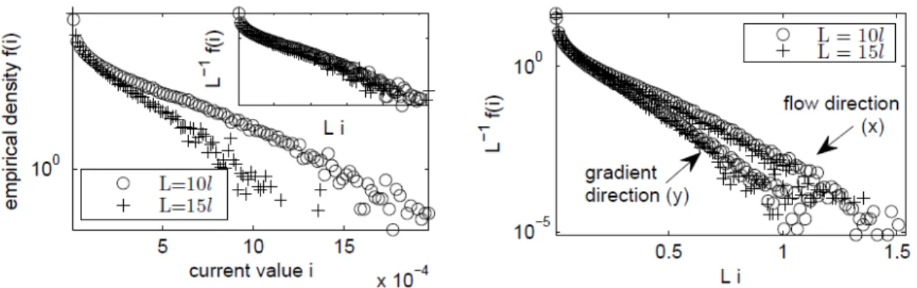
Figure 2.2. Left: current distributions in isotropic dispersions (Pe=0) at rod volume fraction θ = 1.33%. Two system sizes are considered: 10 times as long as a rod (L= 10l) and 15 times as long as a rod (L= 15l). The inset shows the same distributions rescaled by the system size L withu = 1 and v = 1. Right: rescaled current distributions in the flow direction (x) and in the flow gradient direction (y) in sheared (Pe=5) dispersions at rod volume fractionθ = 1.5%. It demonstrates that the finite size scaling holds in each direction under shear . . . 10
Figure 2.3. Multi-scale electrical properties across the percolation phase diagram (Figure 4.11). The top row shows the color-coded average bulk conductivities in the flow (x) direction (left panel), flow-gradient (y) direction (center panel), and vorticity (z) direction (right panel). The bottom row shows the rates of the exponential current tails in the three physical directions respectively . . . 11
Figure 3.1. Charge can be stored at the conductor plates in a vacuum as in the left panel. However, when dielectric material is placed between the plates, additional charge is stored . . . 16
Figure 3.2. In the toy example, there are only three perfect conductors . . . 17
Figure 3.3. The red curve is the dielectric constant for nano-composite system, where the rods are parallel to each other and perpendicular to the plates. We measure the direction from major principal axis. The green curve is for the isotropic distribution . . . 19
Figure 3.4. Given shear rate 60, we measured the dielectric tensor from x,y and z directions . . . 20
Figure 3.5. This figure is from Fig.2 of Simoes et al. [1] . . . 21
Figure 3.6. Electric field in between the plates . . . 21
Figure 3.7. A randomly oriented (P e = 0) dispersion of aspect ratio 20 rods at volume fraction 0.05% . . . 22
Figure 3.8. Rods are parallel with each other, while parallel to the plates (left panel) and perpendicular to the plates (right panel) . . . 22
Figure 3.9. The plates are 10mm×10mm, separated by a 1.75mm gap. 25 metallic particles, with individual particle volume the same as a sphere with radius 0.25mm, were placed between the plates. The orientation and the aspect ratio of the particles were varied . . . 24
Figure 3.10. We verify the calculation of capacitance calcuation in this figure. The symbols show numerical results, the solid lines theory from Eqn 3.15 and Eqn 3.16 . . . 24
Figure 4.1. Shear flow is imposed to the system with velocity field: v = Pe(y, 0, 0), i.e., the direction of flow is along the x axis, with y axis the flow gradient direction and z the vorticity direction . . . 28
Figure 4.2. Plots of sample points drawn from f(m, t) viewed from top (left column) and viewed from side (right column) at 4 shear rates, from no shear (Pe=0) to strong shear (Pe=10). Each subplot contains 3000 points . 30
Figure 4.3. The solid lines represent the theoretical results from asymptotic analysis. The blue, red green color represents isotropic oriented, shear rate 50 and perpendicular to the plates respectively. Upper triangle, lower triangle and star means x, y, z direction. The aspect ratio is 10 with 20 realizations for each point . . . 34
Figure 4.4. The left panel: the normalized dielectric enhancement when shear rate Pe=0.2, while right panel is the log-log plot of the first plot. Each plot is an average of 50 realizations . . . 34
Figure 4.5. The left panel: the normalized dielectric constant when shear rate Pe=35, AR=10 in three principal direction in a box whose length and gap is 10 and 1.5 times rods length respectively. Each point is an average of 50 realizations. The right panel: Anisotropy dielectric constant v.s. normalized shear rate . . . 35
Figure 4.6. For various Peclet numbers, the dielectric constant relative to volume fraction in three principal directions. The black lines are the lower and upper bounds for the dielectric constant, corresponding to uniform rod alignment either orthogonal or parallel to the plates. Moreover the upper triangles, dots and the lower triangles represent the principal direction and two minor directions respectively. In this figure, the aspect ratios are AR=10 . . . 36
Figure 4.8. Anisotropic Dielectric slope is plotted against normalized Peclet number as the three colored lines for different principal axes. The scaling slopes are estimated from the linear fitting to the mean dielectric constant enhancement in each direction. A 95% confidence interval is shown as a shaded region around each slope. The dashed lines are fittings using Eq.4.5. Aspect ratio AR= 10 . . . 38
Figure 4.9. The scaling of the dielectric constant in three different principal axis directions against rods concentration. The left panel: Percolation phase diagram with anisotropic percolation thresholds in the 2-parameter space of (Pe, θ) ( Figure 4 in [2]). . . 39
Figure 4.10. With isotopic Dispersion, we show the dielectric constant v.s. volume fraction for AR=10 (the blue line) and AR=20(the red line) respectively. Here the box length is 7 time the rod’s length with 30 realizations . . . 40
Figure 4.11. Multi-scale electric and dielectric properties across the percolation phase diagram. It shows the color-coded average bulk conductance (upper panel) and dielectric constant(lower panel)). Here aspect ratio AR=10 with box length 7 times the rods length. Each shear rate and volume fraction has 20 realizations . . . 41
Figure 5.1. The equivalent circuit of a three-particle system . . . 45
Figure 5.2. Different color indicates different system size. The distribution of pair-wise charge is plotted according to its volume fraction. This plot is an average of 500 realizations, Pe=0, aspect raio=20. The volume fraction in left panel is 0.2% while for the right panel it is 0.3% . . . 46
Figure 5.3. Different color indicates different volume fraction. The distribution of pair-wise charge is plotted according to its volume fraction. This plot is an average of 500 realizations . . . 47
Figure 5.4. Different color indicates different system size. The distribution of pair-wise charge is plotted according to its volume fraction. This plot is an average of 500 realizations . . . 48
Figure 5.5. Scaling of the first 6 sample moments with respect to the system size L. The bond density is fixed at volume fraction = 0.25 and the system size L varies from 4 to 7. The fitted equations of the moments Mk are shown
in the figure (cf. Equation 5.3)). Curves are normalized. This plot is an average of 500 realizations . . . 49
Figure 5.6. Rescaled pairwise charge distributions in the flow direction(x) and in the flow gradient direction (y) in sheared (Pe = 60) dispersions at rod volume fraction = 0.2%. It demonstrates that the finite size scaling form Equation 5.3 holds in each direction under shear . . . 50
Figure 6.1. A randomly oriented (P e = 0) dispersion of aspect ratio 20 rods at volume fraction 0.05 %. The external voltage is applied to the two dark blue plates . . . 53
Figure 6.2. For the same set of parameters and isotropic dispersion configurations, our results about breakdown voltage are compared with [3]. A statistical description of the network is obtained by an average of 30 realizations . . . . 56
Figure 6.3. For isotropic dispersion, aspect ratio AR=10,each point is an average of 10 configurations . . . 56
Figure 6.4. For aspect ratio AR=10,each point is an average of 5 configurations.The break-down voltage has linear trend with the shortest path between sink and source . . . 57
Figure 6.5. For aspect ratio AR=10,each point is an average of 30 configurations.The shear-rate-60 configuration requires higher breakdown voltage than the isotropic system . . . 58
Figure 7.1. Edge weights are power flows, with darker colors denoting larger values. Node colors represent community identities. Most lines between communities are carrying larger power flow than those inside communities do. Furthermore, one could merge the each community to a ?big node? and do contingency analysis on the new network topology . . . 62
Figure 7.2. x label indicates each transmission line, while the y label shows the comparision between our score and the performance index . . . 64
Figure 7.3. We firstly apply reduction to this power grid network system. And then we sort the transmission lines according to our contingency analysis method. The x direction represents the performance index computed from exact calculation, while the y axis shows the score defined in this section. From the figure, only few points appear in the fourth quadrant, which indicates the most significant transmission lines are well captured by the our score . . . 64
Figure 7.4. The x direction represents the performance index computed from exact calculation, while the y axis shows the score defined in this section. The power grid network is composed of several components and our method works well one component. However this component captures the most important edges and indicates that he most significant transmission lines are well captured by the our score . . . 65
CHAPTER 1: INTRODUCTION
1.1. Background
Components in complex physical systems range from as large as generators in power grids, to as small as nano-particles particles in modern nano-composite material design. A sig-nificant effort in the engineering, scientific and social science communities has focused on the interplay between network structure and dynamics on the network, no matter what the dynamic properties may be(social activity, electrical current or charge).Pursued collectively in Statistical Physics, Applied Mathematics, Computer Science, and Social Science etc., the interdisciplinary study of such diverse systems using network represen-tations and detection algorithms has been exploded during the past two decades [5–8].
The internet could be modeled as a huge network of computers and routers, an ex-ample of a scale-free network [9, 10].In biology, the nervous or the brain system can be modeled as a network of neurons and neural fibers [11–14]. The power grid system, as a network, consists of generators as nodes and transmission lines as edges [4].
Motivated by these successful applications of network analysis in complex systems, my research focuses on the development of new novel network models and corresponding theories that enable previously undetected insights into the structure and dynamics of complex systems. At the ame time, my work seeks to advance network analysis tools which provide approaches to coherently articulated questions in real-world complex sys-tems such as nano-composites.
The papers by Watts[15] and Barabasi[9] are typically identified as launching modern era of network science. It was discovered that regardless of their form, size, nature, and origin, most real networks that have been observed in nature and science are driven by a common set of fundamental laws and organizing rules. Network science utilizes the conceptual framework of graph theory and probability, the tools and principles of statistical physics, the computing algorithms from computer science, and tools from statistics and other subjects to help us understand various systems in nature, society, and technology. This feature will be amplified in this thesis on the study of nanocomposites. Numerical simulations reveal previously undetected behavior of these complex systems, and abstract mathematical models such as lattice models from graph theory provide insights into those systems and help us better understand the fundamental structures.
The first part of the thesis studies the network formed by conductive nanorods in nano-materials, and focuses on the dielectrical response of the composite to the structural properties of the network. The second part studies the electrical properties of nanorod-composites and the third part studies power grid.
So motivated, the dissertation focuses on the development of new network models and tools which enable insights into the structure and dynamics of various systems, and seeks to advance network algorithms which provide approaches to coherently articulated questions in real-world complex systems such as composite materials and power grid system.
1.2. Overview of the Dissertation
properties. Some of the work in the four chapters has been published in [16–18], and the remainder is in preparation for journal submission.
The third part(Chapter 7) studies the electrical properties in power-grid systems.
CHAPTER 2: ELECTRIC PROPERTIES OF NANOROD COMPOSITES The contents of this chapter are first authored by my fellow graduate student Feng Shi, and is published in [18]
2.1. Introduction
Conducting nanorods dispersed in poorly or non-conducting matrices at extremely low, O(1%), volume fractions induce gains in bulk conductivities. The remarkable feature
shear film flow. We then use network representations and graph algorithms to filter the rod ensemble to only current carrying rods, and then solve Kirchoff’s laws on the perco-lating cluster. We average Monte Carlo realizations at each point in the phase diagram, and then analyze the multi-scale electrical properties. We find compelling evidence or robust exponential scaling in the large current tails across all percolation domains, i.e., in isotropic and highly anisotropic rod orientational distributions, independent of the direc-tions or dimensions of percolation. We further show the exponential scaling in the large currents extends more broadly across the current distribution above threshold, whereas the celebrated power law scaling in the small current tail at criticality quickly disinte-grates. These results are remarkably consistent with recent results of the authors for the model system of lattice bond percolation in random resistor networks Shi et al., [18].
2.2. Model and Methods
Here we study Brownian nanorod dispersions where contact percolation occurs well be-low the nematic transition (see [19], for example). Externally imposed shear induces anisotropic rod orientations which are reflected in the local and bulk properties carried by anisotropic percolating paths. Modeling single-particle electrical response by effec-tive resistance proportional to path length, we statistically assess multi-resolution (local and bulk) electrical properties of a highly conducting rod particle phase dispersed in a relatively very poorly conducting matrix phase.
Our first step is to calculate the rod orientational probability distribution function (PDF) of a sheared nanorod dispersion by numerically solving the Doi-Hess-Smoluchowski equation which takes into account the effects of Brownian motion and particle-particle interactions. We refer to Forest et al. [20] for the kinetic theory and attractor phase diagrams of the nanorod orientational distributions versus rod volume fraction θ and normalized shear rate or Peclet number Pe. These orientational distributions arise from imposed simple shear with a presumed rapid quench of rod microstructure. For each
θ and Pe we compute the kinetic distribution function, thereby creating a database of distributions across the (Pe, θ) parameter space. (Since it turns out that percolation in the rod phase occurs at volume fractions well below the nematic transition, we focus this study at volume fractions where the unsheared stable equilibrium is isotropic [2]).
The second step populates Monte Carlo (MC) samples of 3D sheared nanorod disper-sions in a cubic box of lengthLat each fixed (Pe,θ), as in Zhenget al. [2]. The nanorods are randomly distributed in space with the orientation of each rod independently drawn from the corresponding orientational distribution. The rods are modeled as cylinders of length l and diameter d with two spherical caps, representing monodisperse soft-core spheroids. Since we do not check for overlap between particles in this step, the Bal-berg formula [21] is adopted to determine the number N of rods for a given rod volume fraction θ:
(2.1) N = ln(1−θ)
−1L3
V ,
whereV is the volume of a single rod. For rods that are partially out of the box, periodic boundary conditions are applied so that the correct rod volume fraction is achieved.
onto the dimensional percolation phase diagram, as visualized in Figure 4.11. We then perform statistical analysis of this database that describes electrical properties in several ways, including visual depictions.
Every MC realization of a 3D nanorod dispersion is mapped to an undirected weighted network to study its linear DC electrical response. Recall that each MC realization distributes rods uniformly in space with orientations drawn from the specified single-particle orientation distribution. Electrically conducting contact between rods is assumed wherever rods overlap, that is, whenever their axes are within one rod diameter. To study percolation and conductance along each of the three physical dimensions, (perfectly) conducting plates are assumed at the two opposite faces of the box orthogonal to the specified dimension, corresponding to imposing a voltage drop across that dimension, with all intersections between rods and the selected boundary taken to be conducting. Working non-dimensionally, we treat each rod to be a conductor with unit conductivity. Then the conductance of a full rod is equal to its cross-sectional area divided by its length. For the purposes of the present model, we treat the matrix/solvent as a perfect insulator, noting that the typical ratio of conductivities is many orders of magnitude. Every node in the corresponding electrical network represents one of the points of electrical contact between two rods or with a conducting plate, with weighted edges specified by the effective conductance between two contacts, inversely proportional to the corresponding distance along the rod connecting the two contact points, as represented by the (symmetric) adjacency matrix A:
Aij =
wij if node i and node j are connected 0 otherwise
with conductanceswij = s/dij given by the rod cross-sectional area,s, and the distance between node i and node j, dij. To investigate electrical conductivity in a specified direction, the conducting end plates placed on the corresponding opposite faces are each represented by a node, connected to one another through an external source.
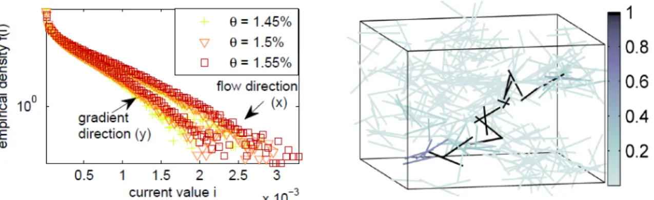
Figure 2.1. Left: current distributions in both the flow direction (x)
and the flow gradient direction (y) for sheared dispersions (Pe=5). The percolation threshold is θc(x)
.
= 1.35% in the flow direction (x) and
θc(y)
.
= 1.4% in the flow gradient direciton (y). Right: visualization of the current-carrying rods and color-coded current values in a percolating cluster from one realization at (Pe,θ)=(10, .015)
2.3. Results and Discussions
The robust exponential tail, which dominates the current distribution above threshold, persists in each spatial direction and is weakly dependent on the rod volume fraction θ
as in the isotropic (Pe=0) case.
The intuition behind the exponential tail is that large currents are very rare, pos-sibly occurring only in the “funnel-shaped” regions [23], while small currents are more abundant. However, a mathematical reasoning for the existence of the exponential tail remains unknown. Importantly, the small numbers of large currents in the tail of the distribution of current-carrying rods exacerbates the separate phenomena of there being relatively few current-carrying rods among the total dispersion, as remarked on above (see Figure [the reduction figure]). To illustrate the combined effect of small numbers of current-carrying rods and even smaller numbers of large currents, Figure 2.1 (right) visualizes the currents flowing from left to right in an example Monte Carlo realization of a 3D sheared dispersion, at (Pe,θ)=(10, .015) and box lengthL= 250 nm, demon-strating how very few of the approximately 10,000 rods initially in this volume carry the large currents.
Figure 2.2. Left: current distributions in isotropic dispersions (Pe=0)
at rod volume fraction θ = 1.33%. Two system sizes are considered: 10 times as long as a rod (L = 10l) and 15 times as long as a rod (L = 15l). The inset shows the same distributions rescaled by the system size L with u = 1 and v = 1. Right: rescaled current distributions in the flow direction (x) and in the flow gradient direction (y) in sheared (Pe=5) dispersions at rod volume fraction θ = 1.5%. It demonstrates that the finite size scaling holds in each direction under shear
Again this simple finite size scaling form remains the same in each direction under shear regardless of the current distribution being anisotropic, as shown in Figure 2.2 (right) which plots the rescaled current distributions f∞ = L−1f
L(L−1i) in both the flow direction (x) and the flow gradient direction (y) for a sheared (Pe=5) dispersion.
Figure 2.3. Multi-scale electrical properties across the percolation phase
diagram (Figure 4.11). The top row shows the color-coded average bulk conductivities in the flow (x) direction (left panel), flow-gradient (y) direc-tion (center panel), and vorticity (z) direcdirec-tion (right panel). The bottom row shows the rates of the exponential current tails in the three physical directions respectively
smaller as shear increases, indicating that large currents are relatively more frequent as shear increases. Whereas in both the flow gradient (y) and the vorticity (z) directions the rates increase with shear rate, indicating that large currents are more rare as shear increases. This observation agrees with the fact that rods tend to align to the x direction as shear increases [20] and hence it is hard to get a “funnel-shaped” region [23] in y and z directions. With knowledge on the exponential current tail, one can show that the largest current in the network scales aslnLand the power-law scaling of the bulk conductivity is inherited from the exponential current tail [24]. These observations are relevant especially to active composite materials where materials are exposed to mechanical loading and strain deformations.
2.4. Conclusion
In summary, we construct a network representation to efficiently and accurately calculate the linear electrical response on percolating anisotropic nanorod dispersions in 3D across the phase diagram of rod volume fraction and imposed normalized shear rate associated with a thin film flow. The dispersions are generated from pre-computed orientational probability distributions across the phase diagram [25, 26]. Network methods provide an efficient algorithm to identify the current-carrying rods in percolating nanorod com-ponents, combining with Monte Carlo calls to the orientational distributions to deliver robust, multi-resolution distributions of conductivity consistent with the statistical prop-erties of the underlying nanorod ensembles. Putting these tools together, we statistically investigate electrical properties on the sheared nanorod percolation phase diagram. This work motivates us to study the dielectric property for the nanocomposite across different shear rate and volume fraction in Chapter 3 and 4.
CHAPTER 3: THE EFFECTS OF SHAPE AND ORIENTATION
3.1. Introduction
We examine the effects of aspect ratio and orientational order of nanoparticles on the dielectric properties of nanocomposites. The motivation is to clearly establish the effects of orientational order, since ambiguities exist in the literature. We focus on metal-lic nanoparticles, and show that, in the dilute concentration limit, theory, experiments and numerical simulations all unequivocally indicate that the effective dielectric con-stant increases with increasing aspect ratio and increasing degree of alignment of rod-like nanoparticles when they orient in the direction of the electric field.
The influence of aspect ratio and anisotropic orientation of nanoparticles on the ef-fective electric conductivities [1], mechanical properties [2, 3], and barrier properties [4] has been investigated experimentally. The influence of aspect ratio [5, 6] and orienta-tion on the dielectric properties has also been studied, but there were inconsistencies in the literature regarding the effects of orientation. Ref. [7] reports an increase in the dielectric constant for field-aligned carbon nanotubes when measured along the field di-rection, Ref. [8] reports nonmonotonic behavior for shear-aligned carbon nanotubes, and calculations for metallic nanorods in Ref. [6] predict a decrease of the dielectric constant with alignment. The motivation for this study is to clarify the influence of aspect ratio and orientation of nanoparticles on the bulk dielectric properties. The goal is to clearly establish normal baseline behavior, which may be useful in interpreting and resolving conflicting reports in the literature.
3.2. Model and Methods
The material under study is placed between two capacitor plates, and, since the ca-pacitance is proportional to the dielectric constant, from the measured caca-pacitance of the capacitor plates, the dielectric constant can be determined. To determine the ca-pacitance, one needs to calculate the potential at the conductor surfaces which act as capacitor plates, here labeledj andk, with given charges±Q. This requires the solution of Laplace’s equation for the potential Φ with the appropriate boundary conditions,
(3.1)
∂Φ
∂ˆt
+
= 0, 0h ∂Φ
∂nˆ
+
=σ(r)
Hereˆt,nˆ denote the tangent and normal directions of the conductor surfaces, includ-ing capacitor plates and conductive particles, and subscripts + implies that the derivative is calculated from outside of the conductor surface, σ(r) is the charge density on the surface of the conductor. One can write the potential at any point in terms of the charge distribution σ(r)
(3.2) Φ(r) = −
M X
i=1 Z
Ci
σ(r0) 4π0h
1
|r−r0|dS,
The method to obtain the dielectric properties is through the capacitance matrix. In general, for an assembly of M conductors in a uniform dielectric, the relation between charge and electric potential can be written as
(3.3) Q= CV
where Qi, the ith element of the vector Q, is the total charge of conductor i, C is the capacitance matrix with elements Ci,j, and Vi, the ith element of the vector V, is the potential of conductor i with respect to ground. Software is readily available to calculate the capacitance matrix. One popular package to calculate the capacitance matrix is FastCap [27]. From the capacitance matrix, one can obtain the desired capacitance between any two conductors. However, the capacitance Cj,k is not trivially related to the elements of the capacitance matrix, rather it can be obtained from the elements of the inverse capacitance matrix as follows.
The capacitance matrix, once obtained, may be inverted to give,
(3.4) Q=BV
where B = C−1 Letting Q
j = Qand Qk = −Q and for all other elements Qi = 0, one has at once ,
(3.5) Vj =BjjQ−Bj, kQ
and
(3.6) Vk =BkjQ−Bk, kQ
It follows that,
(3.7) Cj,k =
1
Bj,j +Bk, k−Bj,k−Bk,j
Figure 3.1. Charge can be stored at the conductor plates in a vacuum
as in the left panel. However, when dielectric material is placed between the plates, additional charge is stored
Once the capacitance is known, the effective permittivity can be calculated from
(3.8) = Cj,k
C0,jk
whereC0,jk is the capacitance between the conductors j and k in free space with no other conductors as in figure 3.1(a).
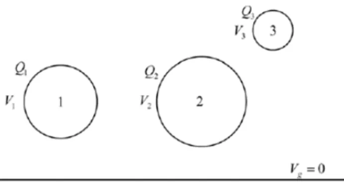
Figure 3.2. In the toy example, there are only three perfect conductors
In this toy example, we study a system with 3 perfect conductors and calculate the dielectric constant of the system.
According to the Kirchoff voltage law, Q=CV, where Q is the charge distribution, V is the voltage distribution and C is the capacitance matrix which could be calculated from FASTCAP [27]. We apply charge Qto the first conductor, and −Qthe third one.
Q = C(1,1)V1+C(1,2)V2+C(1,3)V3 0 = C(2,1)V1+C(2,2)V2+C(2,3)V3 −Q = C(3,1)V1+C(3,2)V2+C(3,3)V3
Therefore the total capacitance in this system is:
(3.9) C1,3 =
Q
V1 −V3
where C1,3 is the pairwise capacitance between capacitor 1 and capacitor 3. Thus the dielectric constant of this system is:
(3.10) C1,3 =
Q
V1 −V3
(3.11) = C1,3
C0,13
Again C0,13 is the capacitance between the conductors 1 and 3 in free space.
The simple theory in the next section and the optical measurements of field alignment experiments in Zheng et al. [17] unequivocally show that, at low volume fractions, the dielectric constant for a nano-composite system increases if the particles align along the field direction. This result is different from the reports in [1, 3] and it also differs from the dependence of electrical conductivity near the percolation threshold.
However, at the early stage of this project, we obtained similar results as the afore-mentioned literatures, which suggested that the problem was not related to a “mistake”, but rather something subtle in the application of the FASTCAP package.
The first challenge is to appropriately interpret the capacitance matrix. In the cal-culation of the dielectric tensor, we obtained the capcitance matrix from FASTCAP[27]. Thus we focus in detail on the capacitance matrix. For a capacitance matrix C, on the diagonal, each matrix element Ci,i is called the self-capacitance of the ith object. Off the diagonal, each matrix element Ci,j is called the mutal capacitance between the ith object and the jth object. Assume the two external plates are the sink and source, then one might try to treat the capacitance of the whole system as Csink,source.
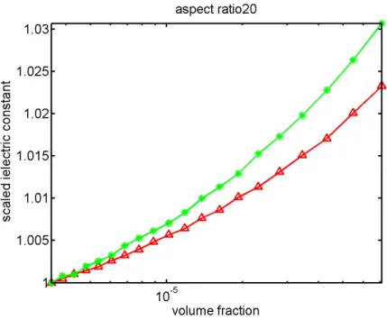
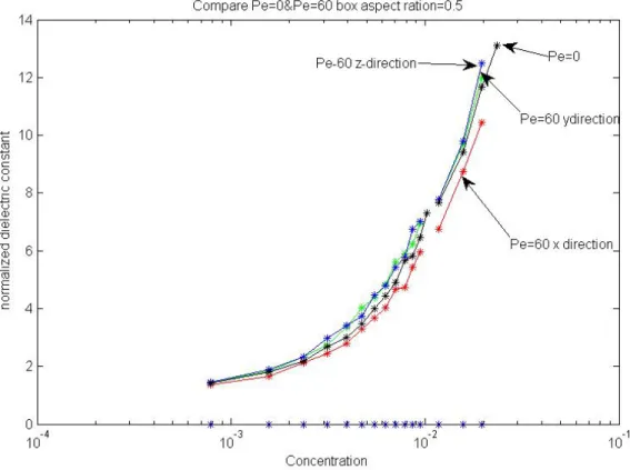
The result in Figure 3.3 and Figure 3.4 shows that for sheared to nanorod composites, the dielectric constant measured along the principal axis of rod orientation is smaller than dielectric constant along any direction in isotropic distribution of the same material, which is consistent with the conclusion shown in Simoes et al [1] figure 3.5.
Figure 3.3. The red curve is the dielectric constant for nano-composite
system, where the rods are parallel to each other and perpendicular to the plates. We measure the direction from major principal axis. The green curve is for the isotropic distribution
use the matrix C, as a whole, connecting the applied charge and voltage distribution in equation 3.2. Specifically, the calculation needs to go through all the steps in section??. The second difficulty in calculating the dielectric tensor is the shape of the plates. Due to finite size effects shown in Figure 3.6, the electric fields will bulge out or fringe out of the plate area. In order to reduce the finite size effects, and make the electric field between the two plates as perpendicular as possible, the idea is to have two infinite plates. However, it is not realistic in the simulation, so we instead assume the length of the plates is at least 10 times larger than the gap.
We begin by considering a continuum model of high-dielectric-constant-inclusion com-posites. The ellipsoid is generated as the inclusion with dielectric constant i, with semi-axis a > b. It could be used to simulate nanorod dispersions when a/b 1.
According to [17], assume mˆ as the unit vector along the symmetry axis, h as dielectric host with relative permittivity, φ as volume fraction. The effective dielectric
Figure 3.4. Given shear rate 60, we measured the dielectric tensor from
x,y and z directions
constant is
(3.12) ef f = h(1 +φ < α1mˆmˆ +α2(I −mˆmˆ)>)
If the dielectric constant of the inclusion is extremely high, i → ∞, then α1 = La1 andα2 = 1−2La, where theLais the depolarization factor given by 2ba
R∞ 0
dx
(x+(a/b)2)3/2(x+1).
The probability density function f is computed through solving the Doi-Hess-Smoluchowski equation of liquid crystalline polymer kinetic theory. Inspired by the conductivity results in [2], we express mˆmˆ in terms of the second moment of the PDF,M =< mˆm >ˆ .
(3.13) ef f =h{1 +φ( 2 1−La
I + ( 1
La
− 2 1−La
Figure 3.5. This figure is from Fig.2 of Simoeset al. [1]
Figure 3.6. Electric field in between the plates
In the extreme cases, the rods are parallel to each other, with the E field along align-ment direction and perpendicular to alignalign-ment direction respectively, and the dielectric constant is given in paper[17].
When rods are isotropically oriented as in fig 3.7, the dielectric tensor remains isotropic spaced, proportional to the identity matrix, M = 13I,
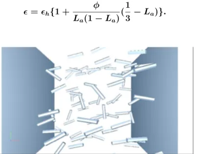
(3.14) = h{1 +
φ
La(1−La) (1
3 −La)}.
Figure 3.7. A randomly oriented (P e= 0) dispersion of aspect ratio 20
rods at volume fraction0.05%
When rods are parallel with each other and parallel to the plates,
(3.15) k =h{1 +
φ
La(1−La)[( 1
3 −La) + 2( 1
3 −La)].}
When rods are parallel with each other but they are perpendicular to the plates,
(3.16) ⊥ =h{1 +
φ
La(1−La) [(1
3 −La)−( 1
3 −La)].}
Figure 3.8. Rods are parallel with each other, while parallel to the plates
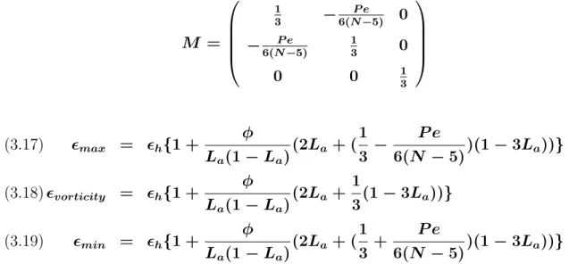
Given a weak shear along the flow or x direction, where the shear rate P e <<1, N is the concentration, according to [2], the second moment matrix is :
M = 1 3 − P e 6(N−5) 0 − P e
6(N−5)
1
3 0
0 0 13
max = h{1 +
φ
La(1−La)
(2La+ ( 1 3 −
P e
6(N −5))(1−3La))} (3.17)
vorticity = h{1 +
φ
La(1−La)
(2La+ 1
3(1−3La))} (3.18)
min = h{1 +
φ
La(1−La)
(2La+ ( 1 3 +
P e
6(N −5))(1−3La))} (3.19)
3.3. Results and Discussion
We have carried out calculations of the capacitance matrix of a parallel plate capacitor with ellipsoidal metallic particles between the plates using FASTCAP. A schematic of our geometry is shown in Fig 3.9.
The plates are10mm×10mm, separated by a1.75mmgap0.25metallic particles, with individual particle volume the same as a sphere with radius0.25mm, were placed between the plates. The orientation and the aspect ratio of the particles were varied.
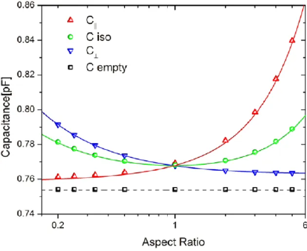
Fig 3.10 shows the dependence of the capacitance for perfectly oriented particles on aspect ratio. The results show that if the alignment direction Nˆ is along the applied field, perpendicular to the capacitor plates, the capacitance increases with aspect ratio, whereas if the alignment direction Nˆ is perpendicular to the applied field, and is parallel to the plates, the capacitance decreases with aspect ratio. This is in agreement with simple theory.
Figure 3.9. The plates are10mm×10mm, separated by a 1.75mm gap.
25 metallic particles, with individual particle volume the same as a sphere with radius 0.25mm, were placed between the plates. The orientation and the aspect ratio of the particles were varied
Figure 3.10. We verify the calculation of capacitance calcuation in this
We have considered the effects of nanoparticle shape and orientation on the effective dielectric constant of nanoparticle composites consisting of spheroidal metallic nanopar-ticles. The results of simple theory, optical measurements of field alignment experiments and numerical simulations are in agreement: they unequivocally show that, in the limit of low densities, the dielectric constant for a system of rod-like particles increases if the particles align along the field direction. This is at variance with reports in the literature [1][3]. This behavior also differs from the dependence of electrical conductivity near the percolation transition. This observation further proved in the experiment session of our paper [17].
3.4. Conclusion
We have considered the effects of nanoparticle shape and orientation on the effective dielectric constant of nanoparticle composites consisting of spheroidal metallic nanopar-ticles. The results of simple theory, optical measurements of field alignment experiments and numerical simulations are in agreement (in Figure 3.10): they unequivocally show that, in the limit of low densities, the dielectric constant for a system of rod-like particles increases if the particles align along the field direction. This is at variance with reports in the literature [1, 3] and this behavior also differs from the dependence of electrical conductivity near the percolation transition.
In the low density regime, well below the percolation threshold, the simple analytic results of Eqs. 3.15 and 3.16 are in good agreement with simulations, and, in one instance, with experimental observations [28]. They may therefore serve as a useful guide to the estimation of the static dielectric properties of nanocomposites consisting of metallic nanoparticles having ellipsoidal shape.
CHAPTER 4: DIELECTRIC TENSOR FOR NANOROD DISPERSIONS
4.1. Introduction
The electrical properties of conductive nanorods dispersed in non-conductive matrices are particularly sensitive to the concentration. It is believed this effect is because of the formation of a network of nanorods forming paths for the electrical current to flow through. In addition to the concentration, aspect ratio (AR) and dispersion are also expected to affect the material response.
Previous work has experimentally studied the influence of concentration, aspect ratio and orientation of nano-particles on the effective electric conductivities [29], and mechan-ical properties [30]. For dielectric properties, [31] reported: when measured along the field direction, the dielectric constant for field-aligned nano-tubes will increase.
However it lacks fundamental theory to understand the underlying phenomena due to the complexity of the problem. As a result, a fast algorithm can provide useful insights. The authors of [17] proposed a method of calculating the dielectric properties through the capacitance matrix. They investigated the aspect ratio and orientation effects ib the dielectric constant in very small system. The papers [1, 3] introduced a numerical network-based procedure to calculate the composite dielectric constant in nematic case, however, they are using sequential packing algorithm to decide the location of the rods, and the scaling behavior of the nematic configuration has not been validated by the experiment.
realistic models allowing rod-rod touch and using the true shear rate computed from polymer kinetic theory. The goal is to establish the effects of volume fraction given the real shear rate and aspect ratio. Network clustering tools are employed to efficiently identify the physically connected component and reduce the system size, which enables us to analyze higher volume fraction. As going to higher volume fraction towards percolation threshold, the theory is not valid and a phase transition could be observed. Meanwhile, we are also interested in the scaling behavior of the charge distribution for equivalent circuit of the nano-system.
4.2. Model and Methods
Assume the orientation of a rod by its axis of symmetry mand the probability distribu-tion funcdistribu-tion (PDF) for its orientadistribu-tion by f(m, t). The dynamics of f(m, t) in a flow field v satisfy:
∂f
∂t +v ·Of = R·[D
0
r(Rf + 1
kTf RV)]−R·[m×mf˙ ]
(4.1)
˙
m = Ω·m+ [D·m−D : mmm] (4.2)
where D0
r is the rotary diffusivity; k is the Boltzmann constant; T is absolute tempera-ture; R is the rotational gradient operator; and V is the mean-field, Maier-Saupe excluded volume potential:
V = −3
2N kT mm: M
M = < mm >= Z
kmk=1
mmf(m, t)dm
Figure 4.1. Shear flow is imposed to the system with velocity field: v =
Pe(y, 0, 0), i.e., the direction of flow is along the x axis, with y axis the flow gradient direction and z the vorticity direction
The imposed flow v is a simple shear (Figure 4.1) with x being the flow direction, y being the flow-gradient direction, and z being the vorticity direction:
v(x, y, z) = P e(y,0,0); (4.3)
D and ω are the corresponding rate-of-strain (symmetric) tensor and voticity (antisym-metric) tensor of the flow v.
The solution of 4.1 is well approximated by a spherical harmonic expansion,
f(m, t) = L X
l=0 l X
n=l
al,n(t)Yln(θ, φ)
where Yn
l are complex spherical harmonic functions and (θ, φ) are the spherical coor-dinates of the axis m:
m= (sinθcosφ, sinθsinφ, cosθ).
showed that results are robust for a finite series expansion forL≥ 10. Similarly, in this work Eq. 4.1 is solved by numeric solution of the 65-dimensional ODE system resulting from truncating the spherical harmonic expansion at L = 10.
The distribution of m can be quantitatively characterized by its second moment tensor
M =< mm >=Rkmk=1mmf(m, t)dm. The eigenvector associated with the largest eigenvalue of M corresponds to the principal direction of alignment (i.e., the most likely direction). When Pe = 0 (no shear) the three eigenvalues of M are {1/3,1/3,1/3} and hence the orientation is isotropic. When P e > 0 both asymptotic analysis [2] and numerical calculation [20] show that the largest eigenvector (i.e., the one corresponding to the largest eigenvalue) lies in the x-y plane, pointing approximately 45◦ from the x axis as P e −→ 0+, and moves closer to the x axis as shear increases; the second eigenvector also lies in the x-y plane, and the smallest eigenvector aligns with the z axis (the vorticity direction). These results agree with the observations in Figure 4.2.
3000 sample points are drawn from f(m, t) at different shear rate Pe. The sample points lie on the unit sphere, indicating the direction of m. The figure 4.2 plots the sample points in space viewed from top (left column) and viewed from side (right column) at 4 shear rates, from no shear (Pe=0) to strong shear (Pe=10). As shear increases, nanorods will be more likely to align with the flow direction (x axis), while slightly biased towards the shear direction (y axis) and more orthogonal to the vorticity direction (z axis). This anisotropy in orientation will be reflected in network properties such as anisotropic percolating paths and conductivities.
Figure 4.2. Plots of sample points drawn from f(m, t) viewed from top
Starting from using the numerical solution for Doi-Hess- Smoluchowski equation of polymer kinetic theory, we generate the rods drawn from orientational probability density function for specified rod volume fraction and shear rate based on algorithm in [32]. when the two rods’s axes are within one rod diameter distance, we assume they connect with each other.
For each realization, the configuration is mapped to an undirected weighted network G = (V, E), with nodes representing rods or conducting plate, and unweighted edges specified by the connection between two nodes, as presented by the adjacency matrix A:
Aij =
1 if node i and node j are connected 0 otherwise
To study dielectric constant in a given direction, we place the external plates on the corresponding opposite faces, which are represented by two nodes (sink and source) respectively, connected to one another by an external source. For each network obtained above, we apply the component detection to the adjacency matrix to efficiently identify the connected components. Note that all the rods in the same connected component share the same voltage here with,in the absence of current, that is, they can be grouped into one conductor when calculating the capacitance and voltage distribution, which significantly reduces the size of the system and improves numerical precision especially in the highly sensitive small voltage.
The dielectric response of this reduced network is given by Kirchoffs voltage law CV = Q, where Q is a vector consisting of the net charge on each node, V is a vector indicating the voltage at each node, and C is the capacitance matrix of the network computed by FASTCAP [27]. Assuming the applied voltage is less than the dielectric breakdown threshold and ignoring electron tunneling effects, for all internal nodes i, Qi = 0, while
Qsource = Q and Qsink = −Q at the two nodes representing the source and sink at oppositely facing end plates.
The bulk dielectric constant is the ratio of the capacitance of the capacitor using nano-particles as a dielectric, compared to a similar capacitor that has a vacuum as its dielectric, where the capacitance is the ratio of the external charge to the obtained voltage drop across the two plate nodes. Naturally, if the two virtual nodes are connected by a percolating path, the bulk dielectric constant in this model is zero.
For each fixed (Pe,θ), a physical 3D realization of the nanorod dispersion is created, with orientations drawn from the kinetic orientational distribution [32]. Without loss of generality, the shear is chosen to be along x-axis, with the flow gradient along y-axis and the vorticity along z axis. We consider a system of nanorods dispersed in an box with the side length of plate at least five times the gap length, which ensures the electric field direction be perpendicular to the plates. The model was tested for consistency, providing the dielectric constant independent of system size given the same box-ratio.
Next we get the corresponding dielectric property in each of the three principal axes for each realization, computing the bulk dielectric constant tensor for each realization. At each specified (Pe, θ), 50 Monte Carlo realizations are generated, and a statistical description of the dielectric property is obtained by an average of these realizations.
We summarize our algorithm as follows:
Algorithm ◦ Provide the property of constituents
◦ Solve Hydrodynamic model of rods under shear
◦ With the numerical solution in previous step, generate the orientational PDF
◦Generate the Nanorod dispersions using Monte Carlo Simulation based on the
◦ Combine with network model and calculate the Dielectric Properties
properties including bulk dielectric constant and local charge distribution. Now given all the input, the first thing we need to figure out is the orientation of rods. Prof. Forest and collaborators [26] [25] [20] have worked out a kinetic model for the motions of rods under shear flow. Although rod orientation is not in equilibrium, we can solve this model numerically to get the distribution of rod orientation. Then we can proceed in a Monte Carlo fashion. To get one sample of this kind of material, first we put nanorod uniformly in a box, and then for each rod its orientation is drawn from the orientational pdf we have. Finally we map this sample to an electrical network and solve the electrical problem on it. After we get enough samples, we can obtain a statistical description of the system. There are two things about this algorithm which distinguish it from other algorithms. First we have a realistic distribution for the orientation of rods. The second is: network model and tools reduce the size of the problem greatly so we can use existing numerical solver to deal with real problem.
4.3. Results and Discussions
In order to study the effect of shear, we plot the dielectric constant tensor in both the major principal axis and two minor axes as the green curves of Figure 4.3. The scaling behavior of dielectric tensor of the dilute region is shown in Figure 4.3. The two perpendicular configurations are lower and upper bounds of the dielectric constant respectively. The theoretical results of the perpendicular and isotropic systems derived in Equation 3.15 and Equation 3.16 agree with the numerical simulation.
Figure 4.3. The solid lines represent the theoretical results from
asymp-totic analysis. The blue, red green color represents isotropic oriented, shear rate 50 and perpendicular to the plates respectively. Upper triangle, lower triangle and star means x, y, z direction. The aspect ratio is 10 with 20 realizations for each point
Figure 4.4. The left panel: the normalized dielectric enhancement when
In Figure 4.4, the upper triangle line is measured from the major principle axis, the lower one is from the minor principal axis, while the middle one is along the vorticity direction. The order of the lines in the simulation is exactly the same as the one in the theory. So for the extremely smallP e, the theory results are confirmed by the numerical simulation.
Figure 4.5. The left panel: the normalized dielectric constant when shear
rate Pe=35, AR=10 in three principal direction in a box whose length and gap is 10 and 1.5 times rods length respectively. Each point is an average of 50 realizations. The right panel: Anisotropy dielectric constant v.s. normalized shear rate
Next, we are interested in arbitrarily strong shear, where P e 1. To elucidate the effect of strong shear on the scaling of dielectric constant enhancement, we firstly take the horizontal slice and vertical slice in the left panel of Figure 4.5. Figure 4.5 shows the mean bulk dielectric constant enhancement in each of the three principal directions against rod volume fraction and Peclet number, which demonstrates the effect of shear to be anisotropic.
In figure 4.7, different shear rates are examined. Firstly, Figure 4.7 suggests that the dielectric constant measured along the major principal axis of nanorod orientation provides an upper bound for fixed shear rate and volume fraction. The implication is: the direction of the principal axis is the eigenvector of the largest eigenvalue of the second moment of PDF, matrix M. This direction is of maximum degree of mesoscopic alignment. Each shear rate, the dielectric constant scales linearly with volume fraction
Figure 4.6. For various Peclet numbers, the dielectric constant relative to
volume fraction in three principal directions. The black lines are the lower and upper bounds for the dielectric constant, corresponding to uniform rod alignment either orthogonal or parallel to the plates. Moreover the upper triangles, dots and the lower triangles represent the principal direction and two minor directions respectively. In this figure, the aspect ratios are AR=10
Figure 4.7. This figure shows the relationship between dielectric constant
and the volume fraction, with the same notation as Figure 4.7, however, the aspect ratio AR is 20. Thus, regardless of different aspect ratio, the linear trend between dielectric constant and volume fraction always holds
(4.4) ∼ θ∗t(P e)
where the scaling slope t(P e) varies with the principal axes of the orientational distri-bution, i.e., ti(P e), where i labels the principal axes of the PDF.
At each normalized shear rate P e, we fit Eq.4.4 to the mean dielectric constant enhancement in each direction as in Figure 4.7, and plot the scaling slopes in Figure 4.8 against Pe.
Shear enhances dielectric slope in the major principal axis, while diminishing the slope (and hence diminishing the property gains) in the minor axis, with the strongest impact
Figure 4.8. Anisotropic Dielectric slope is plotted against normalized
Peclet number as the three colored lines for different principal axes. The scaling slopes are estimated from the linear fitting to the mean dielec-tric constant enhancement in each direction. A 95% confidence interval is shown as a shaded region around each slope. The dashed lines are fittings using Eq.4.5. Aspect ratio AR= 10
in the major principal axis direction. The slops t(P e) are approximately exponential functions of Pe, as can be fitted from Figure 4.8:
t1 = 0.9−0.29exp(−0.102P e)−0.20exp(−0.0123P e) (4.5)
t2 = 0.05 + 0.171exp(−0.172P e) + 0.22exp(−0.0022P e) (4.6)
Figure 4.9. The scaling of the dielectric constant in three different
princi-pal axis directions against rods concentration. The left panel: Percolation phase diagram with anisotropic percolation thresholds in the 2-parameter space of (Pe, θ) ( Figure 4 in [2]).
Thus far we have considered the dielectric constant to a unit charge source with a finite shear rate. To meaningfully describe the dielectric constant in an infinite large Peclet (P e → ∞) and to better understand the effect of shear on the dielectric constant, we perform a further analysis in Eq. 4.5. The limit of Peclet number shows that the dielectric constant for each principal axis monotonically converges to a plateau where the rods are perpendicular or parallel to the plates, which confirms that these two extreme cases are the upper bound and lower bound.
Figure 4.9 shows the average bulk dielectric constant in the major principal direction. At higher volume fraction approaching the percolation threshold, the effective dielectric constant fails to match with the theory, and a super-linear curve is observed. The blue triangles represent the isotropic dispersion, while the other symbols show the transition behavior of dielectric constant in three principal axis directions for P e = 60. Along the major principal axis, the dielectric constant is larger than in the isotropic case for small volume fraction. As the volume fraction goes higher, isotropic’s dielectric constant exhibit a shaper transition. Here aspect ratio AR=10(left panel) AR=20(right panel) with box length 7 times the rods length and 30 realizations.
Figure 4.10. With isotopic Dispersion, we show the dielectric constant
v.s. volume fraction for AR=10 (the blue line) and AR=20(the red line) respectively. Here the box length is 7 time the rod’s length with 30 real-izations
While the low-volume fraction and small-shear rate behavior is well predicted by the theory, little is known about the scaling behavior of the large region of volume fraction and stronger shear. We focus here on the higher volume fraction, figure 4.9 shows the dielectric constant no longer scales linearly with volume fraction and thereby signals a breakdown in the asymptotic theory.
Figure 4.11. Multi-scale electric and dielectric properties across the
per-colation phase diagram. It shows the color-coded average bulk conduc-tance (upper panel) and dielectric constant(lower panel)). Here aspect ratio AR=10 with box length 7 times the rods length. Each shear rate and volume fraction has 20 realizations
to have higher dielectric constant with the same volume fraction. When approaching the percolation threshold, the dielectric constant for both curves increase dramatically, reaching almost the same value.
To conclude, we paint the average bulk dielectric constant and the rates of the bulk conductivities onto the percolation phase diagram
In Figure 4.11, from left to right, the top three panels in the figure show the color-coded average bulk dielectric constant in the flow (x) direction, flow-gradient (y) direc-tion, and vorticity (z) direction respectively; and the bottom three panels show the rates
of the conductivities in those three directions. The effect of shear on the dielectric con-stant and conductivities are similar while shear has relatively smaller impact in the flow (x) direction.
When impose shear to the system (Figure 4.11), it might store charge in one direction while be conductive in other directions. For the lower panel, the system loses finite dielectric constant dimension by dimension, which is a dual problem of the conductance (lower panel in Figure 4.11). In such a capacitor-conductance hybrid device, one function relies on electrostatic charge storage in one direction as a battery, and other function relies on the conductivity in other direction as a resistor.
4.4. Conclusion
In this section, we have considered the effects of nanoparticle shape and orientation on the effective dielectric constant of nanoparticle composites consisting of spheroidal metallic nanoparticles. The theoretical model for dielectric constant is developed as an extension of the conductance model in Zheng et al. [2], and these results are published in [17]. We construct a network representation to efficiently and accurately calculate the linear dielectrical response on anisotropic nanorod dispersions in 3D across different rod volume fraction and imposed normalized shear rate associated with a thin film flow. The dispersions are generated from pre-computed orientational probability distributions across the phase diagram [20, 25, 26, 32]. Network methods, combining with Monte Carlo calls to the orientational distributions provide an efficient algorithm to identify the dielectric properties of the underlying nanorod ensembles.
experiments and numerical simulations are in agreement: they show that, in the limit of low densities, the dielectric constant for a system of rod-like particles increases if the particles align along the field direction as in Figure 4.3 and Figure 4.4. This is at variance with reports in the literature [1, 3] and this behavior also differs from the dependence of electrical conductivity near the percolation transition. Putting these tools together, we statistically investigate dielectrical properties on the sheared nanorod percolation phase diagram. For each data point in the phase diagram, we determine the mean of the bulk dielectric constant, which has a dual shape of the phase diagram for conductivity as in figure 4.11.
We show that there is a linear trend (Figure 4.7) between dielectric constant and the volume fraction across all shear rate. We further provide a universal scaling formula for the coefficient of the linear shape in Figure 4.8.
Furthermore, we paint the dielectric constant and conductivity on the phase-diagram (in Figure 4.11) across different shear rate and volume fraction, which indicates the dual behavior of these two properties. In future work, such data may motivate study of the hybrid material storing charge from one direction while conducting in other direction.
CHAPTER 5: PAIRWISE CHARGE DISTRIBUTION
5.1. Introduction
Current distributions and their scaling behavior have fundamental importance in ma-terials science. Low moments of the current distribution dictate physically measurable properties, e.g., the second moment describes the bulk conductance [18]. Another illus-tration is in the study of breakdown of random media [34].
Shiet al.[16] reveals the dominating extent of an exponential large current tail, which controls macroscopic properties such as the scaling behavior of the largest current and the power-law scaling of the bulk conductivity.
This chapter is motivated by the work [16]. We analyze the pairwise charge distri-bution, showing the exponential large charge tail. It then takes moments to show the robustness of the exponential tail which is independent of the volume fraction given a unit average electric field in the system.
5.2. Model and Methods
Figure 5.1. The equivalent circuit of a three-particle system
5.3. Results and Discussion
Little is known or has been reported about the large pairwise charge tail of the distri-bution even though the large pair-wise charge dominate bulk properties. Figure 5.2 suggests an exponential tail of the charge distribution. Because the charge split up mul-tiplicatively at rods, it is expected to get lots of pairs that carry tiny charges. On the other hand, it is rare to generate configurations which contain large charge, therefore, the charge distribution tail is relatively sharp. This general shape appears to persist as system size goes up.
Figure 5.2. Different color indicates different system size. The
distribu-tion of pair-wise charge is plotted according to its volume fracdistribu-tion. This plot is an average of 500 realizations, Pe=0, aspect raio=20. The volume fraction in left panel is 0.2%while for the right panel it is 0.3%
This section focuses on the large pairwise-charge tail, revealing a robust exponential distribution below or close to percolation threshold. Despite slightly larger noise at left panel of figure 5.2, the straight lines at both rods densities point to exponential tails of the pairwise charge distributions, and the rate of the exponential decay increases with the system size L. Figure 5.3 demonstrates the exponential tail doesn’t depend on the scaling form of the tail of the charge distribution and the volume fraction. In order to better understand the effect of system size on the pairwise charge distribution, we carry out a finite-size scaling analysis on the distributions. LetfL(q) be the probability density function (PDF) of the pairwise change at system size L for unit charge source and f∞(q) is a function independent of L by properly re-scaling fL(i) with L, we aim to eliminate the effect of the system size:
The rate of the exponential decay increases with the system size L. Through tuning the parameters, we confirm that the densities for different system sizes collapse onto a single curve with the relation:
Figure 5.3. Different color indicates different volume fraction. The
dis-tribution of pair-wise charge is plotted according to its volume fraction. This plot is an average of 500 realizations
wheref∞(q)is a function independent of L. By tuning u and v we aim to eliminate the effect of system size. In a finite system the pair-wise charge density for a unit voltage source scales as:
(5.2) fL(q) = 1
Lf ∞
(qL)
Empirical probability density function of the charge in an rod system at rods in isotropic dispersions (P e = 0) at rod volume fraction 0.2% (the left panel of Figure
Figure 5.4. Different color indicates different system size. The
distribu-tion of pair-wise charge is plotted according to its volume fracdistribu-tion. This plot is an average of 500 realizations
5.4) for various system sizes L. A constant unit voltage is imposed across the system. The plot is derived from the histograms of all the pairwise charge over 500 realizations.
The right panel of figure 5.4 confirms that the PDFs for different system sizes collapse onto a single curve when rescaled by the equation 5.3.
However, the simple scaling form in equation 5.3 is not trivial. It implies that the mul-tifractal property of the pairwise charge distribution comes from small pairwise-charge, since the large pairwise-charge tail has a simple scaling form with respect to the system size. Specifically, the kth moment Mk of the large charge described by this finite-size scaling is a simple scaling function of L:
(5.3) Mk =
Z ∞
0
qkfL(q)dq = Z ∞
0
qk1 Lf
∞
(qL)dq ∝ L−(k+2)
To confirm this simple scaling form of the moments, the first several sample moments. The sample moments are calculated as Mk = N1
P
Figure 5.5. Scaling of the first 6 sample moments with respect to the
system size L. The bond density is fixed at volume fraction = 0.25 and the system size L varies from 4 to 7. The fitted equations of the momentsMk are shown in the figure (cf. Equation 5.3)). Curves are normalized. This plot is an average of 500 realizations
large moments the exponential tail of the charge distribution becomes dominant and thus the scaling relationship approaches Equation 5.3.
Again this simple finite size scaling form Equation 5.3 remains the same in each direction under shear regardless of the pairwise charge distribution being anisotropic, as shown in Figure 5.6 which plots the rescaled charge distributionsf∞(q) = LfL(L−1q) in both the flow direction (x) and the flow gradient direction (y) for a sheared (Pe = 60) dispersion.
Figure 5.6. Rescaled pairwise charge distributions in the flow
direc-tion(x) and in the flow gradient direction (y) in sheared (Pe = 60) dis-persions at rod volume fraction = 0.2%. It demonstrates that the finite size scaling form Equation 5.3 holds in each direction under shear
5.4. Conclustion
In summary, we show a robust exponential tail in the pairwise-charge distribution through-out the nano-rod phase. By large scale simulations and finite size scaling analysis, we identified this behavior to be universal, regardless of system size. In the low-volume regime below percolation threshold, it is precisely this range of pairwise charge that is most relevant for describing and diagnosing the macroscopic dielectrical response for materials applications.
CHAPTER 6: DIELECTRIC BREAKDOWN
6.1. Introduction
In this section, we describe a three dimensional model for dielectric breakdown, allow-ing random position of center of mass for the nano-rods and physical rods orientations based on the calculation in Forest et al. [20]. We then apply the network model to simply the problem and discuss the breakdown dynamics for this model by defining local breakdowns, global breakdown, breakdown field in both isotropic and anisotropic sys-tems. Finally, we define the external voltage for these systems, which we will show as an indicator of the formation of percolation path. Previous papers have built models to simulate low volume fraction system in ideal isotropic systems. Our objective is to extend this work to efficiently obtain the dielectric properties in more realistic systems.
6.2. Model and Method
We assume that breakdown occurs only between the pair of conductors which has E(electrical field) bigger than the Ec( breakdown electrical field). We then define a local breakdown as the formation of an electrical connection between two conductors resulting in those two conductors sharing charge and attaining the same electrical potential.
Using the same criterion for breakdown, we continue this sequence of local breakdowns by increasing the external voltage step by step, storing the external voltage. The sample is broken down completely when a sink-to-source conducting connection is made. The conducting path would then rapidly discharge the capacitor plates.
The present model represents an extension and modification of the capacitor plate model [3]. The charge density of the filler is approximated by cylinders, which has been validated for single wall nanotubes [38]. The N-body problem the charge distribution can be formulated as a simple capacitance extraction problem solved by FASTCAP [27, 39]. It can be solved using graph theory, which is a mathematical abstraction and an efficient method for analyzing paths and networks.

![Figure 3.5. This figure is from Fig.2 of Simoes et al. [1]](https://thumb-us.123doks.com/thumbv2/123dok_us/8231130.2182066/32.918.176.761.115.591/figure-figure-fig-simoes-et-al.webp)